This paper was converted on www.awesomepapers.org from LaTeX by an anonymous user.
Want to know more? Visit the Converter page.

Detecting Fermi Surface Nesting Effect for Fermionic Dicke Transition by Trap Induced Localization

Shi Chen Graduate School of China Academy of Engineering Physics, Beijing, 100193, China    Yu Chen ychen@gscaep.ac.cn Graduate School of China Academy of Engineering Physics, Beijing, 100193, China
Abstract

Recently, the statistical effect of fermionic superradiance is approved by series of experiments both in free space and in a cavity. The Pauli blocking effect can be visualized by a 1/2 scaling of Dicke transition critical pumping strength against particle number NatN_{\rm at} for fermions in a trap. However, the Fermi surface nesting effect, which manifests the enhancement of superradiance by Fermi statistics is still very hard to be identified. Here we studied the influence of localized fermions on the trap edge when both pumping optical lattice and the trap are presented. We find due to localization, the statistical effect in superradiant transition is enhanced. Two new scalings of critical pumping strength are observed as 4/34/3, and 2/32/3 for mediate particle number, and the Pauli blocking scaling 1/31/3 (2d case) in large particle number limit is unaffected. Further, we find the 4/34/3 scaling is subject to a power law increasing with rising ratio between recoil energy and trap frequency in pumping laser direction ER/ωxE_{R}/\omega_{x}. The divergence of this scaling of critical pumping strength against NatN_{\rm at} in ER/ωxE_{R}/\omega_{x}\rightarrow\infty limit can be identified as the Fermi surface nesting effect. Thus we find a practical experimental scheme for visualizing the long-desired Fermi surface nesting effect with the help of trap induced localization in a two-dimensional Fermi gas in a cavity.

Introduction In recent decades, the developments in achieving strong coupling between atoms and light have led us to a new platform for studying non-equilibrium open quantum systemsEsslinger07 ; Colombe07 . With these accumulation, the Dicke model, a typical model of strong interactions between atoms and light is finally realizedEsslinger10 . It ends the era for Dicke transition being purely theoreticalDicke54 ; Lieb73 . The Dicke transition manifests itself through the emergence of the steady state superradiance together with a checkerboard density order in atomsEsslinger11 . The spontaneity of the self-organized crystalline is verified by the roton mode softening Roton12 and the critical behavior of the dynamical structure factorEsslinger13 ; Hemmerich14 ; Esslinger15 . Exotic phases like density-ordered Mott insulatorsHemmerich15ex ; Esslinger16 ; Esslinger18 ; Esslinger20 , as well as supersolid breaking U(1) symmetry and translation symmetry ContinousSS17 ; EsslingerSS17 ; EsslingerSS18 are observed successively experimentally. Excited topics with the combinations of quantum many-body systems and the traditional presentation of an open quantum system — cavity-QED (quantum electrodynamics) are enlightened following these new advancesReview21 .

Besides the developments in the superradiance of Bose gases, there are also many interesting statistical effects in fermionic superradiance. The most prominent signature for Dicke transitions of degenerate Fermi gases is its density dependence, namely, the Fermi surface nesting effect and the Pauli blocking effectSimons14 ; Piazza14 ; Yu14 . The Fermi surface nesting effect is due to the resonance between pairs of nested states on the Fermi surface whose momentum difference matches the cavity photon momentum. It results a sharp decreasing of critical pumping strength at specific fillings. The Pauli blocking effect, on the other hand, leads to a suppression of superradiance due to both of the momentum states connected by photon absorption being occupied. There are also further effects like liquid-gas like a transition for p-band fillingSimons14 and statistical crossover in interacting Fermi gasesYu15 , etc. For a long-time, these studies for statistical effects in fermionic superradiance are only theoretical. In a recent experiment, a steady state superradiance of fermions is realized in a cavity for the first time. A scaling law of critical pumping strength as Nat1/2N^{-1/2}_{\rm at} against the particle number NatN_{\rm at} at large NatN_{\rm at} limit is verified in a three-dimensional trapped fermions systemWu21 . This is in sharp contrast with the bosonic Dicke transition whose scaling law is Nat1N_{\rm at}^{-1}. Pauli blocking effect in free space superradiance is also verified thereafterKetterle21 ; Deb21 ; YeJ21 . Unfortunately, contrary to the well-established Pauli blocking effect, Fermi surface nesting effect, which shows the enhancement of superradiance by Fermi statistics is still not verified in experiment. The main difficulty is the presence of the trap makes density ill-defined.

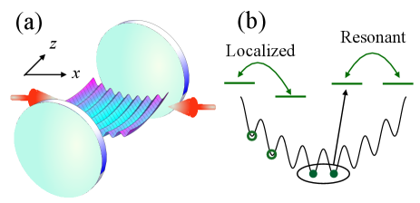
In this Letter, we offer a method to identify the Fermi surface nesting effect for two-dimensional Fermi gases within a trap. We find that, when trap and optical lattice are both presented, there are localized states on the trap edge. The mechanism is shown in Fig. 1(b). One can observe that on the trap edge, the onsite energy difference will outgo the hopping strength, which leads to localization. These localizations then contribute a lot of one-dimensional fermion tubes on the trap edge, where Fermi surface nesting effect is prominent. Phenomenologically, we find for different cavity detune Δc\Delta_{c}, the critical pumping strength of Dicke transition as a function of particle number NatN_{\rm at} falls into two universal functions up to a constant shift in log-log plot. One of the universal curves for small Δc\Delta_{c} shows a universal scaling Nat1N_{\rm at}^{-1} for small NatN_{\rm at} and Nat1/3N_{\rm at}^{-1/3} at large NatN_{\rm at} limit. There is no scaling faster than Nat1N_{\rm at}^{-1} in this typical curve. Let us denote the scaling as ϰ\varkappa for a critical pumping strength scaling law NatϰN_{\rm at}^{-\varkappa} to simplify our description. For larger Δc\Delta_{c}, however, we find a new scaling ϰ>1\varkappa>1 (ϰ=1.33\varkappa=1.33) in intermediate particle number region. We also find a crossover between these two typical critical pumping strength functions, which is sharp within a very small window of Δc\Delta_{c}. In the same crossover Δc\Delta_{c} region, we find the eigenstate on the Fermi surface turns from an extended state to a localized state, which identifies the mechanism. Further, ϰ\varkappa\rightarrow\infty in ωz/ER0\omega_{z}/E_{R}\rightarrow 0 limit at a specific NatN_{\rm at} is obtained as a result of Fermi surface nesting whose tendency is verified numerically. Therefore, the measurement of critical pumping strength as a function of particle number NatN_{\rm at} for different cavity detune Δc\Delta_{c} and different trap frequencies can help us to identify Fermi surface nesting effect. We also stress that the trap induced localization is vital in detecting Fermi surface nesting effect, quite opposite from the original impression of trap being nothing but an obstacle.

Refer to caption
Figure 1: In (a), we show the illustration of our setup. Two-dimensional Fermi gases are put into a cavity with a harmonic trap in xx and zz directions. In (b), we show the mechanism for localization on the trap edge. At the bottom of the trap, fermions at neighbor sites are resonant, thus Bloch state is still a good approximation. On the edge of the trap, the on-site energy difference becomes larger than the hopping strength, which leads to localization.

Model We consider spinless fermions trapped inside a high-Q single mode cavity within a harmonic trap(=1\hbar=1 throughout),

H^\displaystyle\hat{H} =\displaystyle= H^atΔca^a^,\displaystyle\hat{H}_{at}-\Delta_{c}\hat{a}^{{\dagger}}\hat{a}, (1)
H^at=𝑑rψ^(r)(H^0+η(r)(a^+a^)+U0(r)a^a^)ψ^(r),\displaystyle\hat{H}_{at}=\int d\textbf{r}\hat{\psi}^{{\dagger}}(\textbf{r})(\hat{H}_{0}+\eta(\textbf{r})(\hat{a}^{{\dagger}}+\hat{a})+U_{0}(\textbf{r})\hat{a}^{{\dagger}}\hat{a})\hat{\psi}(\textbf{r}), (2)
H^0=22m+VP(r)+12mω2r2,\displaystyle\hat{H}_{0}=\frac{-\nabla^{2}}{2m}+V_{P}(\textbf{r})+\frac{1}{2}m\omega^{2}\textbf{r}^{2}, (3)

Here a^\hat{a} is the annihilation operator of the cavity field, ψ^\hat{\psi} is an annihilation operator of fermionic atoms. Here VP(r)=VPcos2(k0x)V_{P}(\textbf{r})=V_{P}\cos^{2}(k_{0}x) is the optical lattice generated by the pumping field, U0(r)=U0cos2(k0z)U_{0}(\textbf{r})=U_{0}\cos^{2}(k_{0}z) is the cavity field self-energy, η(r)=η0cos(k0x)cos(k0z)\eta(\textbf{r})=\eta_{0}\cos(k_{0}x)\cos(k_{0}z) is the interference between the pumping field and the cavity field. To be more specific, VP=Ωp2/ΔaV_{P}=\Omega^{2}_{p}/\Delta_{a}, U0=g02/ΔaU_{0}=g_{0}^{2}/\Delta_{a}, and η0=gΩp/Δa\eta_{0}=g\Omega_{p}/\Delta_{a}, where Δa=ωaωp\Delta_{a}=\omega_{a}-\omega_{p} is AC stark shift (ωa\omega_{a} is the excited state energy), Δc=ωpωc\Delta_{c}=\omega_{p}-\omega_{c} is the cavity detuning. Here the cavity in consideration has a photon decay rate of κ\kappa. Ωp\Omega_{p} is the strength of the pumping lasers, g0g_{0} is the single-photon Rabi frequency of the cavity field, and k0k_{0} is the wave number of the pumping field which is close to the wave number of the cavity field. The wave number of the cavity field is approximated by k0k_{0}. The recoil energy is defined by ERk02/2mE_{R}\equiv k_{0}^{2}/2m.

Mean Field Theory Since the cavity photon is lossy, the equation of cavity photon field should follow Lindblad equation,

ita^=[a^,H^]+2κa^a^,\displaystyle i\partial_{t}\hat{a}=[\hat{a},\hat{H}]+2\kappa{\cal L}_{\hat{a}}\hat{a}, (4)

where a^a^=a^a^a^12{a^a^,a^}{\cal L}_{\hat{a}}\hat{a}=\hat{a}^{\dagger}\hat{a}\hat{a}-\frac{1}{2}\{\hat{a}^{\dagger}\hat{a},\hat{a}\} is the Lindblad operator on cavity field operator a^\hat{a}. Assuming that the cavity field is in a coherent state |α|\alpha\rangle, such that α|a^|α=α\langle\alpha|\hat{a}|\alpha\rangle=\alpha. Then the above equation can be written as

tα\displaystyle\partial_{t}\alpha =i(η0Θ+(Δc+iκ)α),\displaystyle=i(-\eta_{0}\Theta+(\Delta_{c}^{\prime}+i\kappa)\alpha), (5)

where the effective detuning Δc(α)=Δc𝑑rU(r)n(r)\Delta_{c}^{\prime}(\alpha)=\Delta_{c}-\int d\textbf{r}U(\textbf{r})n(\textbf{r}) and Θ(α)=𝑑rn(r)η(r)/η0\Theta(\alpha)=\int d\textbf{r}n(\textbf{r})\eta(\textbf{r})/\eta_{0}. The fermionic density function is n(r)ψ^(r)ψ^(r)=Tr(ψ^(r)ψ^(r)ρ^(t))n(r)\equiv\braket{\hat{\psi}^{{\dagger}}(\textbf{r})\hat{\psi}(\textbf{{r}})}={\rm Tr}(\hat{\psi}^{{\dagger}}(\textbf{r})\hat{\psi}(\textbf{{r}})\hat{\rho}(t)). Here Tr{\rm Tr} is over the atom’s Hilbert space and a coherent state of cavity field is assumed. Here we assume the steady state density matrix of atoms is ρ^st=eβH^at(α)/Z\hat{\rho}_{\rm st}=e^{-\beta\hat{H}_{at}(\alpha)}/Z (Z=Tr(eβH^at(α))Z={\rm Tr}(e^{-\beta\hat{H}_{at}(\alpha)})), which is justified by a full dynamical handling by Keldysh contour method. Here, H^at(α)\hat{H}_{at}(\alpha) is defined by replace a^\hat{a} in H^at\hat{H}_{at} with α\alpha. In the steady state, α/t=0\partial\alpha/\partial t=0, we have

α=η0Θ(α)Δc(α)+iκ,\displaystyle\alpha=\frac{\eta_{0}\Theta(\alpha)}{\Delta_{c}^{\prime}(\alpha)+i\kappa}, (6)

As α\alpha is complex, the above steady state equation is indeed two equations. If we assume the Dicke transition is a second order transition, then =𝑑𝐫U(𝐫)n(𝐫)U0N/2{\cal B}=\int d{\bf r}U({\bf r})n({\bf r})\approx U_{0}N/2. The phase of α\alpha is locked by κ\kappa. The other equation can be understood as a minimization of free energy α{\cal F}_{\alpha},

αβ1logTr(eβH^at(α)).\displaystyle{\cal F}_{\alpha}\equiv-\beta^{-1}\log{\rm Tr}(e^{-\beta\hat{H}_{at}(\alpha)}). (7)

One can check η0Θ+α𝑑𝐫U(𝐫)n(𝐫)=α/α\eta_{0}\Theta+\alpha\int d{\bf r}U({\bf r})n({\bf r})=\partial{\cal F}_{\alpha}/\partial\alpha^{*}. Then the steady state equation become,

α/αΔcα=0.\displaystyle\partial{\cal F}_{\alpha}/\partial\alpha^{*}-\Delta_{c}\alpha=0. (8)

Further we can find in the second-order expansion of α{\cal F}_{\alpha}, α=η02χ(α+α)2+αα{\cal F}_{\alpha}=-\eta^{2}_{0}\chi(\alpha+\alpha^{*})^{2}+{\cal B}\alpha^{*}\alpha. χ=𝑑𝐫𝑑𝐫δn(𝐫)η(𝐫)δn(𝐫)η(𝐫)/η02\chi=\int d{\bf r}d{\bf r^{\prime}}\langle\delta n({\bf r})\eta({\bf r})\delta n({\bf r^{\prime}})\eta({\bf r}^{\prime})\rangle/\eta^{2}_{0} is the static structure factor, which characterizes the density fluctuation at momentum ±k0𝐞x+±k0𝐞z\pm k_{0}{\bf e}_{x}+\pm k_{0}{\bf e}_{z}.

χ=12η02n,n|𝑑rϕn(r)ϕn(r)η(r)|2nF(En)nF(En)EnEn.\displaystyle\chi=\frac{1}{2\eta^{2}_{0}}\sum_{n,n^{\prime}}\left|\int d\textbf{r}\phi^{*}_{n}(\textbf{r})\phi_{n^{\prime}}(\textbf{r})\eta(\textbf{r})\right|^{2}\frac{n_{F}(E_{n})-n_{F}(E_{n}^{\prime})}{E_{n^{\prime}}-E_{n}}. (9)

Here ϕn(𝐫)\phi_{n}({\bf r}) is the eigenstate of H^0\hat{H}_{\rm 0}, EnE_{n} is the corresponding eigen energy of state |n|n\rangle, nFn_{F} the Fermi distribution function. If we assume the Dicke transition is second order transition, the critical pumping strength is obtained on condition that Δc+4η02χΔc2/(Δc2+κ2)=0\Delta^{\prime}_{c}+4\eta^{2}_{0}\chi\Delta^{\prime 2}_{c}/(\Delta^{\prime 2}_{c}+\kappa^{2})=0 for the second order coefficient of α\alpha in α{\cal F}_{\alpha} being zero. The critical pumping strength is

|VPcr(Nat)ER|=(Δc2+κ2)ER4U0Δcχ(Nat).\displaystyle\left|\frac{V_{P}^{cr}(N_{at})}{E_{R}}\left|=\frac{-(\Delta_{c}^{\prime 2}+\kappa^{2})E_{R}}{4U_{0}\Delta_{c}^{\prime}\chi(N_{\rm at})}\right.\right.. (10)

In this Letter, we will focus on the scaling of VPcrV_{\rm P}^{\rm cr} over NatN_{\rm at} to identify the statistical effect in fermionic superradiance transition in zero temperature.
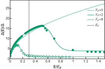
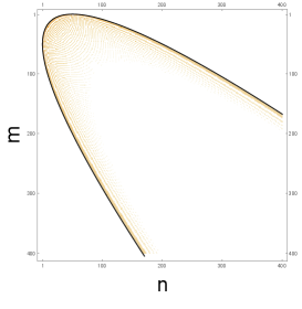
Refer to caption
Figure 2: The width Δ(E)\Delta(E) of different eigenstates of H^y\hat{H}_{y} for different V0V_{0}. Δ=πk0\Delta=\frac{\pi}{k_{0}} is lattice spacing. Black dashed line represent typical fermi energy in our set-up.

Localization on Trap Edge In previous calculation for fermions in a trap, we have assumed that the fermions states are more close to plane wave. However, on the edge of the trap, the interplay between the pumping lattice and the trap can lead to localization. Here we show the mechanism in a two-dimensional non-interacting fermions in a two-dimensional trap.

H^0=x22m+VP(x)+mω022x2z22m+mω022z2\displaystyle\hat{H}_{\rm 0}=-\frac{\partial_{x}^{2}}{2m}+V_{P}(x)+\frac{m\omega_{0}^{2}}{2}x^{2}-\frac{\partial_{z}^{2}}{2m}+\frac{m\omega_{0}^{2}}{2}z^{2} (11)

The eigenstate |n|n\rangle can be factorized as ϕnx(x)ϕnz(z)\phi_{n_{x}}(x)\phi_{n_{z}}(z). ϕnz(z)\phi_{n_{z}}(z) is the eigenstate of Harmonic trap, and its eigen-energy is nzω0n_{z}\omega_{0}. =1\hbar=1. Further, we solve the x direction hamiltonian with the trap, with u1,kx(x)u_{1,k_{x}}(x) being the lowest band Bloch wave function. Then we can construct a Wannier basis by

wj(x)=𝑑kxeikxjdu1,kx(x),w_{j}(x)=\int dk_{x}e^{-ik_{x}jd}u_{1,k_{x}}(x), (12)

where jj is the site index, d=πk0d=\frac{\pi}{k_{0}}. In the Wannier basis, the hamiltonian in x direction can be rewritten as

H^x=x22m+12mω2x2+VPcos2(k0x)=jμj|jj|+t|jj+1|+t|jj1|,\begin{split}\hat{H}_{x}&=-\frac{\partial_{x}^{2}}{2m}+\frac{1}{2}m\omega^{2}x^{2}+V_{P}\cos^{2}(k_{0}x)\\ &=\sum_{j}\mu_{j}\ket{j}\bra{j}+t\ket{j}\bra{j+1}+t\ket{j}\bra{j-1},\end{split} (13)

where, t=𝑑xwi(x)(x22m+Vpcos2(k0x))wi+1(x)t=\int dxw_{i}(x)(-\frac{\partial^{2}_{x}}{2m}+V_{p}\cos^{2}(k_{0}x))w^{*}_{i+1}(x), μi=𝑑y|wi(x)|212ω2x2\mu_{i}=\int dy|w_{i}(x)|^{2}\frac{1}{2}\omega^{2}x^{2}. Next-to-nearest neighbor hopping can be also included, which is not explicitly shown in above equation.

One can check that when |μj+1μj|>t|\mu_{j+1}-\mu_{j}|>t, the eigen-state is localized because the resonance condition between sites is broken down. Here we employ the wave packet width to quantitatively characterize the localization degree of these eigenstates for different eigen-energy. The width of a state is defined as:

Δ(En)=x2nxn2,\displaystyle\Delta(E_{n})=\sqrt{\langle x^{2}\rangle_{n}-\langle x\rangle_{n}^{2}}, (14)

where x2n=𝑑xx2|ϕn(x)|2\langle x^{2}\rangle_{n}=\int dxx^{2}|\phi_{n}(x)|^{2}, xn=𝑑xx|ϕn(x)|2\langle x\rangle_{n}=\int dxx|\phi_{n}(x)|^{2}. In Fig.2, we show Δ(En)\Delta(E_{n}) as a function of excitation energy EnE_{n} for different pumping lattice strengths for fixed trap frequency. A clear sign for mobility edge is shown, and the high energy states can not be approximated as extended states. In the following, we will explore the physical consequences by the trap edge localization.
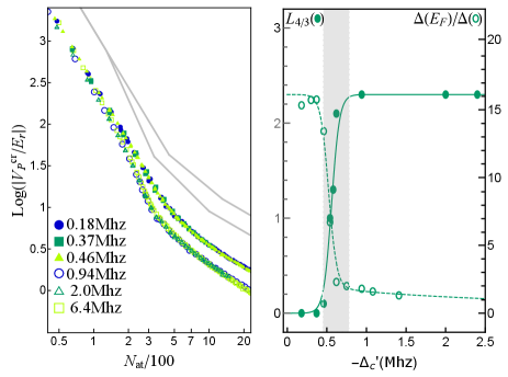
Refer to caption
Figure 3: We fix κ=1MHz,U0=100Hz\kappa=1MHz,U_{0}=-100Hz. In (a), we show the critical pumping strength of the Dicke transition as a function of NatN_{\rm at} for different Δc\Delta_{c}. In (b), the dashed line show the packet width of state near fermi surface, solid line represent the length with a gradient of 1.33 in fig (a).

Scaling of the Critical Pumping Strength — Following Eq. 9 and Eq. 10, together with the calculation of eigen-state |n=|nx,nz|n\rangle=|n_{x},n_{z}\rangle, we can obtain the numerical result for VPcrV_{P}^{\rm cr} for different Δc\Delta_{c} and particle number NatN_{\rm at}. Here we have fixed ωx=ωz=ER/50\omega_{x}=\omega_{z}=E_{R}/50. One can find when Δc\Delta^{\prime}_{c} is larger, the critical pumping strength is larger, thus the localization effect at the trap edge is larger. The numerical result for critical pumping strength of particle number NatN_{\rm at} for different Δc\Delta^{\prime}_{c} is given in Fig. 3(a). One can find for smaller Δc\Delta^{\prime}_{c}, the log-log plot of VPcr(Nat)V_{P}^{\rm cr}(N_{\rm at}) up to a multiplier constant factor falls into one universal curve. The initial scaling of VPcrV_{P}^{\rm cr} against NatN_{\rm at} is 1-1, then it crosses over to 0.66-0.66 and finally it crosses over to 0.35-0.35 in large NatN_{\rm at} limit. The scaling reduction is due to Pauli blocking effect. One can also find there are no scalings larger than 11, which means we only observe the suppression of superradiance due to Fermi statistics. The situation is suddenly changed when Δc>0.5\Delta^{\prime}_{c}>0.5MHz. We find due to localization on the trap edge, the critical pumping strength function VPcr(Nat)V_{P}^{\rm cr}(N_{\rm at}) fall into a new universal curve. In this new universal curve, the initial small NatN_{\rm at} scaling and the large particle number scaling are the same as the previous universal curve. What is beyond, a new scaling being larger than 11 emerges around the middle range NatN_{\rm at}. This middle range NatN_{\rm at} matches the fermion density for Fermi surface nesting effect. We compared the crossover region of the universal critical pumping strength curve and localization effect shown by the typical width of wave function ϕnx(x)\phi_{n_{x}}(x) at the Fermi level. We find these two regions coincide with each other. Here we define L1.33L_{1.33} as the length of 1.331.33 scaling in VPcr(Nat)V_{P}^{\rm cr}(N_{\rm at}). Therefore we conclude that the Pauli blocking scaling 0.350.35 is not affected by localization and a new scaling 1.331.33 emerges due to localization effect. Thus we find the evidence of Fermi surface nesting effect can be magnified by localization effect induced by the trap.

To go further, we will now present a theoretical effective theory to understand why the Pauli blocking effect is immune to the localization effect in large NatN_{\rm at} limit and whether the new scaling 1.331.33 can be interpreted as the Fermi surface nesting effect. Before we give our analysis, we will first give our conclusion. The predictions of our effective theory are 1) the large NatN_{\rm at} limit of VPcrV_{P}^{\rm cr} is VPcrN1/3V_{P}^{\rm cr}\propto N^{-1/3} and it is not changed by localization effect; 2) there is a kink at some middle range NatN_{\rm at}, and the critical pumping strength scaling of NatN_{\rm at} becomes divergent before the kink in ωz0\omega_{z}\rightarrow 0 limit. The second phenomenon is a signature of Fermi surface nesting effect.

Now we will present the assumptions of our effective theory. First of all, ϕnz(z)\phi_{n_{z}}(z) is approximated by its large nzn_{z} asymptotic expression ϕnz(z)cos((2nz+1/2)ωzz)\phi_{n_{z}}(z)\sim\cos(\sqrt{(2n_{z}+1/2)\omega_{z}}z) for even nzn_{z} and sin((2nz+1/2)ωzz\sin(\sqrt{(2n_{z}+1/2)\omega_{z}}z for odd nzn_{z}. Although the original approximation is only correct at large nzn_{z} limit, here we take an approximation for every nzn_{z}. Further we drop the constant 1/21/2 and employ kz2=2nzωzk_{z}^{2}=2n_{z}\omega_{z}. Thus nz=|kz|mωz𝑑kz\sum_{n_{z}}=\int\frac{|k_{z}|}{m\omega_{z}}dk_{z} and ϕnz(z)=cos(kzz)\phi_{n_{z}}(z)=\cos(k_{z}z) or sin(kzz)\sin(k_{z}z). Second, in xx direction, if ϕnx(x)\phi_{n_{x}}(x) is localized at x0x_{0}, then ϕnx(x)=δ(xx0)\phi_{n_{x}}(x)=\delta(x-x_{0}). If the wave function is not localized, we apply a local density approximation and ϕnx(x)\phi_{n_{x}}(x) is characterized by both position x0x_{0} and wave vector kxk_{x}. The eigen-energy is εx0,kx=2tcoskx+12ωxx02\varepsilon_{x_{0},k_{x}}=2t\cos k_{x}+\frac{1}{2}\omega_{x}x_{0}^{2}. Here we introduce xMobx_{\rm Mob} as the mobility edge in xx direction. For x<xMobx<x_{\rm Mob}, the wave function ϕnx(x)\phi_{n_{x}}(x) is extended and for x>xMobx>x_{\rm Mob}, the wave function is localized. nx\sum_{n_{x}} is approximated as a phase space integral 𝑑kx𝑑x0\int dk_{x}dx_{0}. With all these approximations, Eq. 9 and Eq. 10 can be calculated analytically and we find VPcrNat1/3V_{P}^{\rm cr}\propto N^{-1/3}_{\rm at} at large NatN_{\rm at} limit irrelevant to the position of xMobx_{\rm Mob}. The detailed calculation is given in supplementary materialsupp and the theoretical prediction is shown in Fig. 4(a) in solid black curve. A kink at Fermi surface nesting atom number can be observed.

Refer to caption
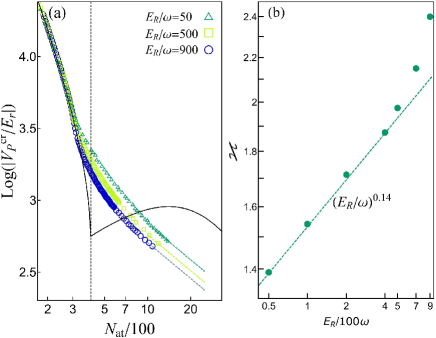
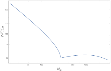
Figure 4: In (a), we show critical pumping strength as a function of particle number for different ωz/ER\omega_{z}/E_{R}. Δc\Delta_{c} is taken in the localized region. One can find when ER/ωzE_{R}/\omega_{z} becomes bigger, the slope in nesting region increases. The gray solid line is the theoretical prediction that we expect as the ER/ωzE_{R}/\omega_{z}\rightarrow\infty limit of the universal critical pumping strength curve. In (b), we show the slope as a function of ER/ωzE_{R}/\omega_{z}. The increase of the slope is found to be faster than power law increasing. As a result, we expect ϰNest\varkappa_{\rm Nest}\rightarrow\infty as ωz/ER0\omega_{z}/E_{R}\rightarrow 0.

Since the approximation in zz direction deviate from reality, we find the approximation is better when ER/ωz1E_{R}/\omega_{z}\gg 1. Therefore we expect the critical pumping strength scaling of NatN_{\rm at} in the middle range NatN_{\rm at} will increase when ωz/ER\omega_{z}/E_{R} is decreasing. Thus this prediction can be numerically checked by numerics. Interestingly, we find except for scaling around the Fermi surface nesting atom number, other scalings of critical pumping strength is invariant for different ωz\omega_{z}. The scaling of critical pumping strength |logVPcr/logNat||\log V_{P}^{\rm cr}/\log N_{\rm at}| is increasing when ωz\omega_{z} is decreasing. We are restricted by the system size and particle number in a numerical calculation, therefore we can only prove that the scaling is increasing when ωz\omega_{z} becomes smaller. A finite size scaling is carried out, and a divergent scaling is obtained in ωz0\omega_{z}\rightarrow 0 limit. All of the present data analysis can be equally done for experimental data. These signatures in critical pumping strength can then be identified as Fermi surface nesting effect.

Conclusion To summarize, we find the Fermi surface nesting effect in fermionic superradiant transition in a cavity can be verified with the help of trap induced localization. We find when the harmonic trap depth is effectively changed, there are two typical curves for superradiant transition critical pumping strength as a function of particle number. For shallow trap without localization effect, there are no signs of Fermi surface nesting, and for tight trap with localization effect, there is Fermi surface nesting signal which manifests as ϰ>1\varkappa>1 for ϰ=log(VPcr)/logNat\varkappa=\log(V_{P}^{\rm cr})/\log N_{\rm at}. We also verified the tendency for ϰ\varkappa\rightarrow\infty in zero trap frequency limit. We find the interplay between trap or localization and superradiance is quite interesting, and statistical effect can be magnified and thus benefits the generation of superradiance.

Acknowledgments.— Y. C is supported by NSFC under Grant No. 12174358 and No. 11734010, and Beijing Natural Science Foundation (Z180013).

References

  • (1) F. Brennecke, T. Donner, S. Ritter, T. Bourdel, M. Köhl, and T. Esslinger, Nature (London) 450, 268 (2007).
  • (2) Y. Colombe, T. Steinmetz, G. Dubios, F. Linke, D. Hunger, and J. Reichel, Nature (London) 450, 272 (2007).
  • (3) K. Baumann, C. Guerlin, F. Brennecke, and T. Esslinger, Nature (London) 464, 1301 (2010).
  • (4) R. H. Dicke, Phys. Rev. 93, 99 (1954).
  • (5) K. Hepp, and E. H. Lieb, Ann. Phys. (N. Y.) 76, 360 (1973).
  • (6) K. Baumann, R. Mottl, F. Brennecke, and T. Esslinger, Phys. Rev. Lett. 107, 140402 (2011).
  • (7) R. Mottl, F. Brennecke, K. Baumann, R. Landig, T. Donner, and T. Esslinger, Science 336, 1570–1573 (2012).
  • (8) F. Brennecke, R. Mottl, K. Baumann, R. Landig, T. Donner, and T. Esslinger, Proceedings of the National Academy of Sciences 110, 11763–11767 (2013).
  • (9) J. Klinder, H. Keβ\betaler, M. Wolke, L. Mathey, and A. Hemmerich, Proceedings of the National Academy of Sciences 112, 3290-3295 (2014).
  • (10) R. Landig, F. Brennecke, R. Mottl, T. Donner, and T. Esslinger, Nature Commun. 6, 7046 (2015).
  • (11) J. Klinder, H. Keßler, M. R. Bakhtiari, M. Thorwart, and A. Hemmerich, Phys. Rev. Lett. 115, 230403 (2015).
  • (12) R. Landig, L. Hruby, N. Dogra, M. Landini, R. Mottl, T. Donner, and T. Esslinger, Nature 532, 476 (2016).
  • (13) L. Hruby, N. Dogra, M. Landini, T. Donner, and T. Esslinger, PNAS 115, 3279 (2018).
  • (14) X. Li, D. Dreon, P. Zupancic, A. Baumgartner, A. Morales, W. Zheng, N. Cooper, T. Donner, and T. Esslinger, Phys. Rev. Res. 3, L012024 (2021).
  • (15) J. Léonard, A. Morales, P. Zupancic, T. Esslinger and T. Donner Nature 543 87-90 (2017).
  • (16) J. Léonard, A. Morales, P. Zupancic, T. Donner, and T. Esslinger, Science 358 1415–1418 (2017).
  • (17) A. Morales, P. Zupancic, J. Léonard, T. Esslinger, and T. Donner, Nature Materials 17 686–690 (2018).
  • (18) F. Mivehvar and F. Piazza and T. Donner and H. Ritsch, Annals of Physics, 70, 1 (2021).
  • (19) J. Keeling, M.J. Bhaseen, and B.D. Simons, Phys. Rev. Lett. 112, 143002 (2014).
  • (20) F. Piazza and P. Strack, Phys. Rev. Lett. 112, 143003 (2014).
  • (21) Y. Chen, Z. Yu, and H. Zhai, Phys. Rev. Lett. 112, 143004 (2014).
  • (22) Y. Chen, H. Zhai, and Z. Yu, Phys. Rev. A 91, 021602(R) (2015).
  • (23) X. Zhang, Y. Chen, Z. Wu, J. Wang, J. Fan, S. Deng, and H. Wu, Science, 373, 1359–1362 (2021).
  • (24) Y. Margalit, Y.-K. Lu, F. C. Top, and W. Ketterle, Science, 374, 976-979 (2021).
  • (25) A. B. Deb, and N. Kjærgaard, Science, 374, 972-975 (2021).
  • (26) C. Sanner, L. Sonderhouse, R. B. Hutson, L. Yan, W. R. Milner, and J. Ye, Science, 374, 979-983 (2021).
  • (27) See supplementary material for the details. In the supplementary material, we include the calculations for the off-diagonal matrix element n|cos(k0z)|n\langle n|\cos(k_{0}z)|n^{\prime}\rangle, and the results for an approximate field theory.

Supplementary Material

Appendix A Calculation of the off-diagonal matrix element n|cos(k0z)|n\langle n|\cos(k_{0}z)|n^{\prime}\rangle in Eq. 9

The transition matrix element n|cos(k0z)|n=𝑑zϕn(z)ϕn(z)cos(k0z)\langle n|\cos(k_{0}z)|n^{\prime}\rangle=\int dz\phi^{*}_{n}(z)\phi_{n^{\prime}}(z)\cos(k_{0}z), ϕn(z)\phi_{n^{\prime}}(z), where ϕn(n)(z)\phi_{n(n^{\prime})}(z) is the eigen-state of harmonic trap in z direction. H^z|n=(z2/2m+(mωzz2)/2)ϕn(z)=ωnzϕn(z)\hat{H}_{z}|n\rangle=(-\partial_{z}^{2}/2m+(m\omega_{z}z^{2})/2)\phi_{n}(z)=\omega_{n}^{z}\phi_{n}(z), ωnz=(n+1/2)ωz\omega_{n}^{z}=(n+1/2)\omega_{z}. =1\hbar=1 is employed. Here we introduce

fnn=n|eik0z|n,\displaystyle f_{nn^{\prime}}=\langle n|e^{ik_{0}z}|n^{\prime}\rangle, (S1)

then we can find that

𝑑zϕn(z)ϕn(z)cos(k0z)=𝑑zϕn(z)ϕn(z)Re(eik0z)=Re(n|eik0z|n)=Re(fnn).\displaystyle\int dz\phi^{*}_{n}(z)\phi_{n^{\prime}}(z)\cos(k_{0}z)=\int dz\phi^{*}_{n}(z)\phi_{n^{\prime}}(z){\rm Re}(e^{ik_{0}z})={\rm Re}(\langle n|e^{ik_{0}z}|n^{\prime}\rangle)={\rm Re}(f_{nn^{\prime}}). (S2)

Since the transition element is just the real part of fnnf_{nn^{\prime}}, therefore we will focus on calculation of fnnf_{nn^{\prime}} in the following. Here we will present an algebraic method involving the annihilation and creation operators. Let us introduce a^=mωz2z+12mωzz\hat{a}=\sqrt{\frac{m\omega_{z}}{2}}z+\sqrt{\frac{1}{2m\omega_{z}}}\partial_{z}, a^=mωz2z12mωzz\hat{a}^{\dagger}=\sqrt{\frac{m\omega_{z}}{2}}z-\sqrt{\frac{1}{2m\omega_{z}}}\partial_{z}, then we have z=12mωz(a^+a^)z=\sqrt{\frac{1}{2m\omega_{z}}}(\hat{a}+\hat{a}^{\dagger}), H^z=ωz(a^a^+12)\hat{H}_{z}=\omega_{z}(\hat{a}^{\dagger}\hat{a}+\frac{1}{2}). Then eigenstate |n=(a^)n/n!|0|n\rangle=(\hat{a}^{\dagger})^{n}/\sqrt{n!}|0\rangle. Then we find

fnn=n|eik0z|n=1n!n!0|a^neik02mωz(a^+a^)(a^)n|0\displaystyle f_{nn^{\prime}}=\langle n|e^{ik_{0}z}|n^{\prime}\rangle=\frac{1}{\sqrt{n!n^{\prime}!}}\langle 0|\hat{a}^{n}e^{i\frac{k_{0}}{\sqrt{2m\omega_{z}}}(\hat{a}+\hat{a}^{\dagger})}(\hat{a}^{{\dagger}})^{n^{\prime}}|0\rangle (S3)

Let us introduce ϑ=k0/2mωz\vartheta=k_{0}/\sqrt{2m\omega_{z}}, then we have

fnn\displaystyle f_{nn^{\prime}} =\displaystyle= n|eik0z|n=1n!n!0|a^neiϑ(a^+a^)(a^)n|0\displaystyle\bra{n}e^{ik_{0}z}\ket{n^{\prime}}=\frac{1}{\sqrt{n!n^{\prime}!}}\langle 0|\hat{a}^{n}e^{i\vartheta(\hat{a}+\hat{a}^{\dagger})}(\hat{a}^{{\dagger}})^{n^{\prime}}|0\rangle (S4)
=\displaystyle= 1n!n!0|eiϑ(a^+a^)eiϑ(a^+a^)a^neiϑ(a^+a^)(a^)n|0.\displaystyle\frac{1}{\sqrt{n!n^{\prime}!}}\langle 0|e^{i\vartheta(\hat{a}+\hat{a}^{\dagger})}e^{-i\vartheta(\hat{a}+\hat{a}^{\dagger})}\hat{a}^{n}e^{i\vartheta(\hat{a}+\hat{a}^{\dagger})}(\hat{a}^{{\dagger}})^{n^{\prime}}|0\rangle.

Making use of Baker-Hausdorff formula, we find

eiϑ(a^+a^)a^neiϑ(a^+a^)=(eiϑ(a^+a^)a^eiϑ(a^+a^))n\displaystyle e^{-i\vartheta(\hat{a}+\hat{a}^{\dagger})}\hat{a}^{n}e^{i\vartheta(\hat{a}+\hat{a}^{\dagger})}=(e^{-i\vartheta(\hat{a}+\hat{a}^{\dagger})}\hat{a}e^{i\vartheta(\hat{a}+\hat{a}^{\dagger})})^{n} (S5)
=\displaystyle= (a^iϑ[a^+a^,a^]+=2(iϑ)![,[a^+a^,a^]])n=(a^+iϑ)n\displaystyle\left(\hat{a}-i\vartheta[\hat{a}+\hat{a}^{\dagger},\hat{a}]+\sum_{\ell=2}^{\infty}\frac{(-i\vartheta)^{\ell}}{\ell!}[\cdots,[\hat{a}+\hat{a}^{\dagger},\hat{a}]\cdots]\right)^{n}=(\hat{a}+i\vartheta)^{n}

Therefore

fnn\displaystyle f_{nn^{\prime}} =\displaystyle= 1n!n!0|eiϑ(a^+a^)(a^+iϑ)n(a^)n|0\displaystyle\frac{1}{\sqrt{n!n^{\prime}!}}\langle 0|e^{i\vartheta(\hat{a}+\hat{a}^{\dagger})}(\hat{a}+i\vartheta)^{n}(\hat{a}^{{\dagger}})^{n^{\prime}}|0\rangle (S6)
=\displaystyle= 1n!0|eiϑ(a^+a^)Cn(iϑ)na^|n\displaystyle\frac{1}{\sqrt{n!}}\langle 0|e^{i\vartheta(\hat{a}+\hat{a}^{\dagger})}\sum_{\ell}C_{n}^{\ell}(i\vartheta)^{n-\ell}\hat{a}^{\ell}|n^{\prime}\rangle

Here we assume nnn\leq n^{\prime}, then we have a^|n=(n!/(n)!)|n\hat{a}^{\ell}|n^{\prime}\rangle=(\sqrt{n^{\prime}!/(n^{\prime}-\ell)!})|n^{\prime}-\ell\rangle. Notice eiϑ(a^+a^)|0e^{-i\vartheta(\hat{a}+\hat{a}^{\dagger})}|0\rangle is a coherent state, denoted as |iϑ|-i\vartheta\rangle. 0|eiϑ(a^+a^)=iϑ|\langle 0|e^{i\vartheta(\hat{a}+\hat{a}^{\dagger})}=\langle-i\vartheta|.

fnn\displaystyle f_{nn^{\prime}} =\displaystyle= 1n!Cn(iϑ)nn!(n)!iϑ|n\displaystyle\frac{1}{\sqrt{n!}}\sum_{\ell}C_{n}^{\ell}(i\vartheta)^{n-\ell}\sqrt{\frac{n^{\prime}!}{(n^{\prime}-\ell)!}}\langle-i\vartheta|n-\ell\rangle (S7)
=\displaystyle= 1n!Cn(iϑ)nn!(n)!1(n)!iϑ|(a^)n|0\displaystyle\frac{1}{\sqrt{n!}}\sum_{\ell}C_{n}^{\ell}(i\vartheta)^{n-\ell}\sqrt{\frac{n^{\prime}!}{(n^{\prime}-\ell)!}}\sqrt{\frac{1}{(n^{\prime}-\ell)!}}\langle-i\vartheta|(\hat{a}^{\dagger})^{n^{\prime}-\ell}|0\rangle
=\displaystyle= n!n!Cn(iϑ)n1(n)!((iϑ))niϑ|0\displaystyle\frac{\sqrt{n^{\prime}!}}{\sqrt{n!}}\sum_{\ell}C_{n}^{\ell}(i\vartheta)^{n-\ell}\frac{1}{(n^{\prime}-\ell)!}((-i\vartheta)^{*})^{n^{\prime}-\ell}\langle-i\vartheta|0\rangle

In the last line of above equation, we have used iϑ|a^=(iϑ)iϑ|\langle-i\vartheta|\hat{a}^{\dagger}=(-i\vartheta)^{*}\langle-i\vartheta|. Finally, we have

fnn\displaystyle f_{nn^{\prime}} =\displaystyle= n!n!=0n(iϑ)n(iϑ)n!(n)!(n)!iϑ|0\displaystyle\sqrt{n^{\prime}!n!}\sum_{\ell=0}^{n}\frac{(i\vartheta)^{n-\ell}(i\vartheta)^{n^{\prime}-\ell}}{\ell!(n-\ell)!(n^{\prime}-\ell)!}\langle-i\vartheta|0\rangle (S8)

The factor iϑ|0\langle-i\vartheta|0\rangle can be calculated as

iϑ|0=0|eik0z|0=1πmωz𝑑zemωzz2eik0z=ek024mωz=e12ϑ2\displaystyle\langle-i\vartheta|0\rangle=\langle 0|e^{ik_{0}z}|0\rangle=\frac{1}{\sqrt{\pi m\omega_{z}}}\int dze^{-m\omega_{z}z^{2}}e^{ik_{0}z}=e^{-\frac{k_{0}^{2}}{4m\omega_{z}}}=e^{-\frac{1}{2}\vartheta^{2}} (S9)

The final result is

fnn=n!n!=0n(iϑ)n(iϑ)n!(n)!(n)!e12ϑ2\displaystyle f_{nn^{\prime}}=\sqrt{n!n^{\prime}!}\sum_{\ell=0}^{n}\frac{(i\vartheta)^{n-\ell}(i\vartheta)^{n^{\prime}-\ell}}{\ell!(n-\ell)!(n^{\prime}-\ell)!}e^{-\frac{1}{2}\vartheta^{2}} (S10)

If n<nn^{\prime}<n, we find

fnn=n!n!=0n(iϑ)n(iϑ)n!(n)!(n)!e12ϑ2\displaystyle f_{nn^{\prime}}=\sqrt{n!n^{\prime}!}\sum_{\ell=0}^{n^{\prime}}\frac{(i\vartheta)^{n-\ell}(i\vartheta)^{n^{\prime}-\ell}}{\ell!(n-\ell)!(n^{\prime}-\ell)!}e^{-\frac{1}{2}\vartheta^{2}} (S11)

In Fig. 5, we show the matrix element of |fnn||f_{nn^{\prime}}| as a function of nn and nn^{\prime}. Meanwhile, in the maintext, we approximate |n|n\rangle as 12(|kz±|kz)\frac{1}{2}(|k_{z}\rangle\pm|-k_{z}\rangle), then fnn=12(δkz,kz+k0+δkz,kzk0)f_{nn^{\prime}}=\frac{1}{2}(\delta_{k^{\prime}_{z},k_{z}+k_{0}}+\delta_{k^{\prime}_{z},k_{z}-k_{0}}). We show the solid line as the delta function between kzk_{z} and kzk^{\prime}_{z}.

Refer to caption
Figure 5: Fixed ϑ=50\vartheta=\sqrt{50}, we show |fmn|2|f_{mn}|^{2} more clearly by matrix density diagram, deep color mean nonzero value. As shown in the figure, when m and n is large, only a small number of points are non-zero, which behave like a dirac function. The black line is the result calculated by approximation  S17 .

Appendix B Predictions of the Effective theory

Considering the fermions in a trap with optical lattice in x direction, the eigenstates are classified into two types. One type is itinerate wave-function and another is localized one. When the excitation energy is above the mobility edge, then the localized eigenstate is labeled by its position in x direction and nzn_{z} in z direction. The energy of eigenstate |j,nz|j,n_{z}\rangle is

ϵj,nz=12mωx2(ja0)2+nzωz,\displaystyle\epsilon_{j,n_{z}}=\frac{1}{2}m\omega^{2}_{x}(ja_{0})^{2}+n_{z}\omega_{z}, (S12)

where a0=π/k0a_{0}=\pi/k_{0} is the lattice length unit. On the other hand, if the eigen energy is smaller than the mobility edge, then we can approximate the excited state energy by local density approximation. ϵj,kx,nz=12mωx2(ja0)2+nzωz+2tcos(kxa0)\epsilon_{j,k_{x},n_{z}}=\frac{1}{2}m\omega^{2}_{x}(ja_{0})^{2}+n_{z}\omega_{z}+2t\cos(k_{x}a_{0}), where tt is the hopping strength in x direction. From this dispersion relation, we can obtain the relation between chemical potential and the particle number NatN_{\rm at}. Here we are going to focus on the case when the localized states are the major states ( this is true when NatN_{\rm at} is large ).

Nat=j,nznF(ϵj,nzμ)=2a002μmωx2𝑑x0μ12mωxx2ωz𝑑nz=43πωxωz2k02mμ3/2\displaystyle N_{\rm at}=\sum_{j,n_{z}}n_{F}(\epsilon_{j,n_{z}}-\mu)=\frac{2}{a_{0}}\int_{0}^{\sqrt{\frac{2\mu}{m\omega_{x}^{2}}}}dx\int_{0}^{\frac{\mu-\frac{1}{2}m\omega_{x}x^{2}}{\omega_{z}}}dn_{z}=\frac{4}{3\pi\omega_{x}\omega_{z}}\sqrt{\frac{2k_{0}^{2}}{m}}\mu^{3/2} (S13)

In above, we usej=Jj=J=1a0Ja0Ja0𝑑x\sum_{j=-J}^{j=J}=\frac{1}{a_{0}}\int_{-Ja_{0}}^{Ja_{0}}dx.Then we can see μNat2/3\mu\propto N_{\rm at}^{2/3}. More explicitly,

μ=(3πωxωz8ERNat)2/3\displaystyle\mu=\left(\frac{3\pi\omega_{x}\omega_{z}}{8\sqrt{E_{R}}}N_{\rm at}\right)^{2/3} (S14)

Now we are going to check the critical pumping strength as a function of chemical potential μ\mu, then equivalently we get the critical pumping strength as a function of NatN_{\rm at} from above relation. From Eq. 10, we know

|VPcr(Nat)ER|=(Δc2+κ2)ER4U0Δcχ(Nat).\displaystyle\left|\frac{V_{P}^{cr}(N_{at})}{E_{R}}\left|=\frac{-(\Delta_{c}^{\prime 2}+\kappa^{2})E_{R}}{4U_{0}\Delta_{c}^{\prime}\chi(N_{\rm at})}\right.\right.. (S15)

where the susceptibility χ\chi is

χ=12η02n,n|𝑑rϕn(r)ϕn(r)η(r)|2nF(En)nF(En)EnEn\displaystyle\chi=\frac{1}{2\eta^{2}_{0}}\sum_{n,n^{\prime}}\left|\int d\textbf{r}\phi^{*}_{n}(\textbf{r})\phi_{n^{\prime}}(\textbf{r})\eta(\textbf{r})\right|^{2}\frac{n_{F}(E_{n})-n_{F}(E_{n}^{\prime})}{E_{n^{\prime}}-E_{n}} (S16)

Attention that the quantum number nn represent all the quantum numbers of the eigenstate, including jj, kxk_{x} and nzn_{z}. Inspired by the asymptotic representation of hermite polynomials: H2nz(z)=(1)nz2nz(2nz1)!!ez2/2[cos(4nz+1z)+O(1nz1/4)]H_{2n_{z}}(z)=(-1)^{n_{z}}2^{n_{z}}(2n_{z}-1)!!e^{z^{2}/2}[\cos{(\sqrt{4n_{z}+1}z)}+O(\frac{1}{n_{z}^{1/4}})], H2nz+1(z)=(1)nz2nz+1/2(2nz1)!!ez2/22nz+1[sin(4nz+3z)+O(1nz1/4)]H_{2n_{z}+1}(z)=(-1)^{n_{z}}2^{n_{z}+1/2}(2n_{z}-1)!!e^{z^{2}/2}\sqrt{2n_{z}+1}[\sin{(\sqrt{4n_{z}+3}z)}+O(\frac{1}{n_{z}^{1/4}})], we can take following approximations for large nzn_{z},

z|2nz12Lkz(z|kz+z|kz)θ(Lkz2z2),\displaystyle\langle z|2n_{z}\rangle\approx\frac{1}{2\sqrt{L_{k_{z}}}}(\langle z|k_{z}\rangle+\langle z|-k_{z}\rangle)\theta(L_{k_{z}}^{2}-z^{2}),
z|2nz+112Lkz(z|kzz|kz)θ(Lkz2z2)(kz>0)\displaystyle\langle z|2n_{z}+1\rangle\approx\frac{1}{2\sqrt{L_{k_{z}}}}(\langle z|k_{z}\rangle-\langle z|-k_{z}\rangle)\theta(L_{k_{z}}^{2}-z^{2})(k_{z}>0) (S17)

where |kz|k_{z}\rangle is a momentum state z|kz=eikzz\langle z|k_{z}\rangle=e^{ik_{z}z},Lkz=π|kz|4mωzL_{k_{z}}=\frac{\pi|k_{z}|}{4m\omega_{z}} and kz2/2m=nzωzk_{z}^{2}/2m=n_{z}\omega_{z}. The range in z direction is due to the wave function is only obvious nonzero within the trap range. Here the plus sign is for nzn_{z} being even and the minus sign is for nzn_{z} being odd. This approximation is good when nzn_{z} is large. But we will take this approximation for all nzn_{z}. Under such approximation, we have

2nz|eik0z|2nz\displaystyle\langle 2n_{z}|e^{ik_{0}z}|2n^{\prime}_{z}\rangle =\displaystyle= 14LkzLkzmin(Lkz,Lkz)min(Lkz,Lkz)𝑑z(kz|+kz|)|zeik0zz|(|kz+|kz)\displaystyle\frac{1}{4\sqrt{L_{k_{z}}L_{k_{z}^{\prime}}}}\int_{-\rm{min}(L_{k_{z}},L_{k^{\prime}_{z}})}^{\rm{min}(L_{k_{z}},L_{k^{\prime}_{z}})}dz(\langle k_{z}|+\langle-k_{z}|)|z\rangle e^{ik_{0}z}\langle z|(|k^{\prime}_{z}\rangle+|-k^{\prime}_{z}\rangle) (S18)

Let us denote Lzmin=min(Lkz,Lkz)L_{z\rm min}={\rm min}(L_{k_{z}},L_{k^{\prime}_{z}}),Lzmax=max(Lkz,Lkz)L_{z\rm max}={\rm max}(L_{k_{z}},L_{k^{\prime}_{z}}). Then we have

2nz|eik0z|2nz\displaystyle\langle 2n_{z}|e^{ik_{0}z}|2n^{\prime}_{z}\rangle =\displaystyle= sin((k0+kzkz)Lzmin)(k0+kzkz)(2LzmaxLzmin)+sin((k0+kz+kz)Lzmin)(k0+kz+kz)(2LzmaxLzmin)+\displaystyle\frac{\sin((k_{0}+k^{\prime}_{z}-k_{z})L_{z\rm min})}{(k_{0}+k^{\prime}_{z}-k_{z})(2\sqrt{L_{z\rm max}L_{z\rm min}})}+\frac{\sin((k_{0}+k^{\prime}_{z}+k_{z})L_{z\rm min})}{(k_{0}+k^{\prime}_{z}+k_{z})(2\sqrt{L_{z\rm max}L_{z\rm min}})}+ (S19)
sin((k0kzkz)Lzmin)(k0kzkz)(2LzmaxLzmin)+sin((k0kz+kz)Lzmin)(k0kz+kz)(2LzmaxLzmin)\displaystyle\frac{\sin((k_{0}-k^{\prime}_{z}-k_{z})L_{z\rm min})}{(k_{0}-k^{\prime}_{z}-k_{z})(2\sqrt{L_{z\rm max}L_{z\rm min}})}+\frac{\sin((k_{0}-k^{\prime}_{z}+k_{z})L_{z\rm min})}{(k_{0}-k^{\prime}_{z}+k_{z})(2\sqrt{L_{z\rm max}L_{z\rm min}})}

Notice that in ωz0+\omega_{z}\rightarrow 0^{+} limit, LzminL_{z\rm min}\rightarrow\infty, such that sin(kLzmin)/kδ(k)\sin(kL_{z\rm min})/k\approx\delta(k). It is easy to check that 2nz|eik0z|2nz=2nz|eik0z|2nz\langle 2n_{z}|e^{-ik_{0}z}|2n^{\prime}_{z}\rangle=\langle 2n_{z}|e^{ik_{0}z}|2n^{\prime}_{z}\rangle, 2nz|cos(k0z)|2nz+1=2nz+1|cos(k0z)|2nz=0\langle 2n_{z}|\cos(k_{0}z)|2n^{\prime}_{z}+1\rangle=\langle 2n_{z}+1|\cos(k_{0}z)|2n^{\prime}_{z}\rangle=0 and 2nz+1|eik0z|2nz+1=2nz+1|eik0z|2nz+1\langle 2n_{z}+1|e^{ik_{0}z}|2n^{\prime}_{z}+1\rangle=\langle 2n_{z}+1|e^{-ik_{0}z}|2n^{\prime}_{z}+1\rangle. What we really need is |2nz|eik0z|2nz|2|\langle 2n_{z}|e^{ik_{0}z}|2n^{\prime}_{z}\rangle|^{2}, we have

|2nz|cos(k0z)|2nz|2\displaystyle\left|\langle 2n_{z}|\cos(k_{0}z)|2n^{\prime}_{z}\rangle\right|^{2} =\displaystyle= (2nz|eik0z|2nz)2\displaystyle(\langle 2n_{z}|e^{ik_{0}z}|2n^{\prime}_{z}\rangle)^{2} (S20)
\displaystyle\approx (sin((k0+kzkz)Lzmin)(k0+kzkz)(2LzmaxLzmin))2+(sin((k0+kz+kz)Lzmin)(k0+kz+kz)(2LzmaxLzmin))2+\displaystyle\left(\frac{\sin((k_{0}+k^{\prime}_{z}-k_{z})L_{z\rm min})}{(k_{0}+k^{\prime}_{z}-k_{z})(2\sqrt{L_{z\rm max}L_{z\rm min}})}\right)^{2}+\left(\frac{\sin((k_{0}+k^{\prime}_{z}+k_{z})L_{z\rm min})}{(k_{0}+k^{\prime}_{z}+k_{z})(2\sqrt{L_{z\rm max}L_{z\rm min}})}\right)^{2}+
(sin((k0kzkz)Lzmin)(k0kzkz)(2LzmaxLzmin))2+(sin((k0kz+kz)Lzmin)(k0kz+kz)(2LzmaxLzmin))2\displaystyle\left(\frac{\sin((k_{0}-k^{\prime}_{z}-k_{z})L_{z\rm min})}{(k_{0}-k^{\prime}_{z}-k_{z})(2\sqrt{L_{z\rm max}L_{z\rm min}})}\right)^{2}+\left(\frac{\sin((k_{0}-k^{\prime}_{z}+k_{z})L_{z\rm min})}{(k_{0}-k^{\prime}_{z}+k_{z})(2\sqrt{L_{z\rm max}L_{z\rm min}})}\right)^{2}
\displaystyle\approx (δkz,kz+k0+δkz,kz+k0+δkz,kz+k0+δkz,kz+k0)/(4Lzmax)\displaystyle\left(\delta_{k_{z},k^{\prime}_{z}+k_{0}}+\delta_{-k_{z},k^{\prime}_{z}+k_{0}}+\delta_{k_{z},-k^{\prime}_{z}+k_{0}}+\delta_{-k_{z},k^{\prime}_{z}+k_{0}}\right)/(4L_{z\rm max})

In the first \approx in above equation, we dropped the cross terms. In the second \approx, we employed limLzmin(sin(kLzmin)/k)2Lzminδ(k)\lim_{L_{z\rm min}\rightarrow\infty}(\sin(kL_{z\rm min})/k)^{2}\approx L_{z\rm min}\delta(k). Meanwhile when we replace nzωzn_{z}\omega_{z} by kz2/2mk_{z}^{2}/2m, the summation over nzn_{z} is replaced by

nz=0𝑑kzkzmωz\displaystyle\sum_{n_{z}}=\int_{0}^{\infty}dk_{z}\frac{k_{z}}{m\omega_{z}} (S21)

By approximation of all the eigenstates are localized, the susceptibility can be written as

χ(μ)\displaystyle\chi(\mu) =12j,nz;j,nz|j,nz|cos(k0z)cos(k0x)|j,nz|2ϵj,nzϵj,nz(θ(μϵj,nz)θ(μϵj,nz))\displaystyle=\frac{1}{2}\sum_{j,n_{z};j^{\prime},n^{\prime}_{z}}\frac{|\langle j,n_{z}|\cos(k_{0}z)\cos(k_{0}x)|j^{\prime},n^{\prime}_{z}\rangle|^{2}}{\epsilon_{j,n_{z}}-\epsilon_{j^{\prime},n^{\prime}_{z}}}(\theta(\mu-\epsilon_{j^{\prime},n^{\prime}_{z}})-\theta(\mu-\epsilon_{j,n_{z}})) (S22)
=12ϵj,nz<μ,ϵj,nz>μ|j,nz|cos(k0z)cos(k0x)|j,nz|2ϵj,nzϵj,nz+12ϵj,nz>μ,ϵj,nz<μ|j,nz|cos(k0z)cos(k0x)|j,nz|2ϵj,nzϵj,nz\displaystyle=\frac{1}{2}\sum_{\epsilon_{j^{\prime},n^{\prime}_{z}}<\mu,\epsilon_{j,n_{z}}>\mu}\frac{|\langle j,n_{z}|\cos(k_{0}z)\cos(k_{0}x)|j^{\prime},n^{\prime}_{z}\rangle|^{2}}{\epsilon_{j,n_{z}}-\epsilon_{j^{\prime},n^{\prime}_{z}}}+\frac{1}{2}\sum_{\epsilon_{j^{\prime},n^{\prime}_{z}}>\mu,\epsilon_{j,n_{z}}<\mu}\frac{|\langle j,n_{z}|\cos(k_{0}z)\cos(k_{0}x)|j^{\prime},n^{\prime}_{z}\rangle|^{2}}{\epsilon_{j,n_{z}}-\epsilon_{j^{\prime},n^{\prime}_{z}}}
=ϵj,nz>μ,ϵj,nz<μ|nz|cos(k0z)|nz|2|j|cos(k0x)|j|2ϵj,nzϵj,nz\displaystyle=\sum_{\epsilon_{j^{\prime},n^{\prime}_{z}}>\mu,\epsilon_{j,n_{z}}<\mu}\frac{|\langle n_{z}|\cos(k_{0}z)|n^{\prime}_{z}\rangle|^{2}|\langle j|\cos(k_{0}x)|j^{\prime}\rangle|^{2}}{\epsilon_{j^{\prime},n^{\prime}_{z}}-\epsilon_{j,n_{z}}}
=ϵj,nz<μ;nz|nz|cos(k0z)|nz|2ϵj,nzϵj,nzθ(ϵj,nzμ)\displaystyle=\sum_{\epsilon_{j,n_{z}}<\mu;n^{\prime}_{z}}\frac{|\langle n_{z}|\cos(k_{0}z)|n^{\prime}_{z}\rangle|^{2}}{\epsilon_{j,n^{\prime}_{z}}-\epsilon_{j,n_{z}}}\theta\left(\epsilon_{j,n^{\prime}_{z}}-\mu\right)

Where |j\ket{j} repersent the state localized in the jth site, now we introduce x=ja0x=ja_{0} Then j=1a0𝑑x\sum_{j}=\frac{1}{a_{0}}\int dx. In these approximations,

χ(μ)\displaystyle\chi(\mu) =1a02μmωx22μmωx2𝑑x2m(μ1/2mωx2x2)2m(μ1/2mωx2x2)|kz|dkz2mωz|kz|dkz2mωz|nz|cos(k0z)|nz|2(nznz)ωzθ(nzωz+mωxx22μ)\displaystyle=\frac{1}{a_{0}}\int_{-\sqrt{\frac{2\mu}{m\omega_{x}^{2}}}}^{\sqrt{\frac{2\mu}{m\omega_{x}^{2}}}}dx\int^{\sqrt{2m(\mu-1/2m\omega_{x}^{2}x^{2})}}_{-\sqrt{2m(\mu-1/2m\omega_{x}^{2}x^{2})}}\frac{|k_{z}|dk_{z}}{2m\omega_{z}}\int\frac{|k^{\prime}_{z}|dk^{\prime}_{z}}{2m\omega_{z}}\frac{|\langle n_{z}|\cos(k_{0}z)|n^{\prime}_{z}\rangle|^{2}}{(n^{\prime}_{z}-n_{z})\omega_{z}}\theta\left(n^{\prime}_{z}\omega_{z}+\frac{m\omega_{x}x^{2}}{2}-\mu\right)
=1a02μmωx22μmωx2𝑑x2m(μ1/2mωx2x2)2m(μ1/2mωx2x2)dkz|kz|2mωz|kz|dkz2mωz(δkz,kzk0+δkz,kzk0+δkz,kzk0+δkz,kzk0)4Lzmax(kz2/2mkz2/2m)\displaystyle=\frac{1}{a_{0}}\int_{-\sqrt{\frac{2\mu}{m\omega_{x}^{2}}}}^{\sqrt{\frac{2\mu}{m\omega_{x}^{2}}}}dx\int^{\sqrt{2m(\mu-1/2m\omega_{x}^{2}x^{2})}}_{-\sqrt{2m(\mu-1/2m\omega_{x}^{2}x^{2})}}\frac{dk_{z}|k_{z}|}{2m\omega_{z}}\int\frac{|k^{\prime}_{z}|dk^{\prime}_{z}}{2m\omega_{z}}\frac{(\delta_{k_{z},k_{z}^{\prime}-k_{0}}+\delta_{k_{z},-k_{z}^{\prime}-k_{0}}+\delta_{-k_{z},k_{z}^{\prime}-k_{0}}+\delta_{-k_{z},-k_{z}^{\prime}-k_{0}})}{4L_{z\rm max}(k^{\prime 2}_{z}/2m-k^{2}_{z}/2m)}
θ(kz22m+mωx2x22μ)\displaystyle\theta\left(\frac{k_{z}^{\prime 2}}{2m}+\frac{m\omega^{2}_{x}x^{2}}{2}-\mu\right)
=1a02μmωx22μmωx2𝑑x2m(μ1/2mωx2x2)2m(μ1/2mωx2x2)|kz|dkz2mωz|kz|dkz2πmax(|kz|,|kz|)\displaystyle=\frac{1}{a_{0}}\int_{-\sqrt{\frac{2\mu}{m\omega_{x}^{2}}}}^{\sqrt{\frac{2\mu}{m\omega_{x}^{2}}}}dx\int^{\sqrt{2m(\mu-1/2m\omega_{x}^{2}x^{2})}}_{-\sqrt{2m(\mu-1/2m\omega_{x}^{2}x^{2})}}\frac{|k_{z}|dk_{z}}{2m\omega_{z}}\int\frac{|k^{\prime}_{z}|dk^{\prime}_{z}}{2\pi\rm{max}(|k_{z}|,|k^{\prime}_{z}|)}
(δkz,kzk0+δkz,kzk0+δkz,kzk0+δkz,kzk0)(kz2/2mkz2/2m)θ(kz22m+mωx2x22μ)\displaystyle\frac{(\delta_{k_{z},k_{z}^{\prime}-k_{0}}+\delta_{k_{z},-k_{z}^{\prime}-k_{0}}+\delta_{-k_{z},k_{z}^{\prime}-k_{0}}+\delta_{-k_{z},-k_{z}^{\prime}-k_{0}})}{(k^{\prime 2}_{z}/2m-k^{2}_{z}/2m)}\theta\left(\frac{k^{\prime 2}_{z}}{2m}+\frac{m\omega^{2}_{x}x^{2}}{2}-\mu\right)
=1a02μmωx22μmωx2𝑑x2m(μ1/2mωx2x2)2m(μ1/2mωx2x2)|kz|dkz2mωz|kz+k0|2πmax(|kz|,|kz+k0|)θ((kz+k0)22m+mωx2x22μ)(kz+k0)2/2mkz2/2m\displaystyle=\frac{1}{a_{0}}\int_{-\sqrt{\frac{2\mu}{m\omega_{x}^{2}}}}^{\sqrt{\frac{2\mu}{m\omega_{x}^{2}}}}dx\int^{\sqrt{2m(\mu-1/2m\omega_{x}^{2}x^{2})}}_{-\sqrt{2m(\mu-1/2m\omega_{x}^{2}x^{2})}}\frac{|k_{z}|dk_{z}}{2m\omega_{z}}\frac{|k_{z}+k_{0}|}{2\pi\rm{max}(|k_{z}|,|k_{z}+k_{0}|)}\frac{\theta\left(\frac{(k_{z}+k_{0})^{2}}{2m}+\frac{m\omega^{2}_{x}x^{2}}{2}-\mu\right)}{(k_{z}+k_{0})^{2}/2m-k_{z}^{2}/2m}
+1a02μmωx22μmωx2𝑑x2m(μ1/2mωx2x2)2m(μ1/2mωx2x2)|kz|dkz2mωz|kz+k0|2πmax(|kz|,|kz+k0|)θ((kz+k0)22m+mωx2x22μ)(kz+k0)2/2mkz2/2m\displaystyle+\frac{1}{a_{0}}\int_{-\sqrt{\frac{2\mu}{m\omega_{x}^{2}}}}^{\sqrt{\frac{2\mu}{m\omega_{x}^{2}}}}dx\int^{\sqrt{2m(\mu-1/2m\omega_{x}^{2}x^{2})}}_{-\sqrt{2m(\mu-1/2m\omega_{x}^{2}x^{2})}}\frac{|k_{z}|dk_{z}}{2m\omega_{z}}\frac{|k_{z}+k_{0}|}{2\pi\rm{max}(|k_{z}|,|k_{z}+k_{0}|)}\frac{\theta\left(\frac{(k_{z}+k_{0})^{2}}{2m}+\frac{m\omega^{2}_{x}x^{2}}{2}-\mu\right)}{(k_{z}+k_{0})^{2}/2m-k_{z}^{2}/2m}
+1a02μmωx22μmωx2𝑑x2m(μ1/2mωx2x2)2m(μ1/2mωx2x2)|kz|dkz2mωz|kzk0|2πmax(|kz|,|kzk0|)θ((kzk0)22m+mωx2x22μ)(kzk0)2/2mkz2/2m\displaystyle+\frac{1}{a_{0}}\int_{-\sqrt{\frac{2\mu}{m\omega_{x}^{2}}}}^{\sqrt{\frac{2\mu}{m\omega_{x}^{2}}}}dx\int^{\sqrt{2m(\mu-1/2m\omega_{x}^{2}x^{2})}}_{-\sqrt{2m(\mu-1/2m\omega_{x}^{2}x^{2})}}\frac{|k_{z}|dk_{z}}{2m\omega_{z}}\frac{|k_{z}-k_{0}|}{2\pi\rm{max}(|k_{z}|,|k_{z}-k_{0}|)}\frac{\theta\left(\frac{(k_{z}-k_{0})^{2}}{2m}+\frac{m\omega^{2}_{x}x^{2}}{2}-\mu\right)}{(k_{z}-k_{0})^{2}/2m-k_{z}^{2}/2m}
=2a02μmωx22μmωx2𝑑x2m(μ1/2mωx2x2)2m(μ1/2mωx2x2)|kz|dkz2mωz|kz+k0|2πmax(|kz|,|kz+k0|)θ((kz+k0)22m+mωx2x22μ)(kz+k0)2/2mkz2/2m\displaystyle=\frac{2}{a_{0}}\int_{-\sqrt{\frac{2\mu}{m\omega_{x}^{2}}}}^{\sqrt{\frac{2\mu}{m\omega_{x}^{2}}}}dx\int^{\sqrt{2m(\mu-1/2m\omega_{x}^{2}x^{2})}}_{-\sqrt{2m(\mu-1/2m\omega_{x}^{2}x^{2})}}\frac{|k_{z}|dk_{z}}{2m\omega_{z}}\frac{|k_{z}+k_{0}|}{2\pi\rm{max}(|k_{z}|,|k_{z}+k_{0}|)}\frac{\theta\left(\frac{(k_{z}+k_{0})^{2}}{2m}+\frac{m\omega^{2}_{x}x^{2}}{2}-\mu\right)}{(k_{z}+k_{0})^{2}/2m-k_{z}^{2}/2m}
+2a02μmωx22μmωx2𝑑x2m(μ1/2mωx2x2)2m(μ1/2mωx2x2)|kz|dkz2mωz|kzk0|2πmax(|kz|,|kzk0|)θ((kzk0)22m+mωx2x22μ)(kzk0)2/2mkz2/2m\displaystyle+\frac{2}{a_{0}}\int_{-\sqrt{\frac{2\mu}{m\omega_{x}^{2}}}}^{\sqrt{\frac{2\mu}{m\omega_{x}^{2}}}}dx\int^{\sqrt{2m(\mu-1/2m\omega_{x}^{2}x^{2})}}_{-\sqrt{2m(\mu-1/2m\omega_{x}^{2}x^{2})}}\frac{|k_{z}|dk_{z}}{2m\omega_{z}}\frac{|k_{z}-k_{0}|}{2\pi\rm{max}(|k_{z}|,|k_{z}-k_{0}|)}\frac{\theta\left(\frac{(k_{z}-k_{0})^{2}}{2m}+\frac{m\omega^{2}_{x}x^{2}}{2}-\mu\right)}{(k_{z}-k_{0})^{2}/2m-k_{z}^{2}/2m}

Noticed that when we change kzk_{z} to kz-k_{z}, the intergred function doesn’t change, so we just need to consider kz>0k_{z}>0.

χ(μ)=\displaystyle\chi(\mu)= 8a002μmωx2𝑑x02m(μ1/2mωx2x2)kzdkz2mωzkz+k02πmax(kz,kz+k0)θ((kz+k0)22m+mωx2x22μ)(kz+k0)2/2mkz2/2m\displaystyle\frac{8}{a_{0}}\int_{0}^{\sqrt{\frac{2\mu}{m\omega_{x}^{2}}}}dx\int^{\sqrt{2m(\mu-1/2m\omega_{x}^{2}x^{2})}}_{0}\frac{k_{z}dk_{z}}{2m\omega_{z}}\frac{k_{z}+k_{0}}{2\pi\rm{max}(k_{z},k_{z}+k_{0})}\frac{\theta\left(\frac{(k_{z}+k_{0})^{2}}{2m}+\frac{m\omega^{2}_{x}x^{2}}{2}-\mu\right)}{(k_{z}+k_{0})^{2}/2m-k_{z}^{2}/2m}
+8a002μmωx2𝑑x02m(μ1/2mωx2x2)kzdkz2mωz|kzk0|2πmax(kz,|kzk0|)θ((kzk0)22m+mωx2x22μ)(kzk0)2/2mkz2/2m\displaystyle+\frac{8}{a_{0}}\int_{0}^{\sqrt{\frac{2\mu}{m\omega_{x}^{2}}}}dx\int^{\sqrt{2m(\mu-1/2m\omega_{x}^{2}x^{2})}}_{0}\frac{k_{z}dk_{z}}{2m\omega_{z}}\frac{|k_{z}-k_{0}|}{2\pi\rm{max}(k_{z},|k_{z}-k_{0}|)}\frac{\theta\left(\frac{(k_{z}-k_{0})^{2}}{2m}+\frac{m\omega^{2}_{x}x^{2}}{2}-\mu\right)}{(k_{z}-k_{0})^{2}/2m-k_{z}^{2}/2m}

The calculation is carried in the three cases:μ/ER<1/4,1/4<μ/ER<1,μ/ER>>1\mu/E_{R}<1/4,1/4<\mu/E_{R}<1,\mu/E_{R}>>1.

For μ<1/4ER\mu<1/4E_{R}, the theta function in χ\chi is always satisfied.

χ(μ)=4μERπ2ωzωx(1+11+ER4μarctan(1/1+ER4μ))\begin{split}\chi(\mu)=\frac{4\sqrt{\mu E_{R}}}{\pi^{2}\omega_{z}\omega_{x}}\left(-1+1\sqrt{-1+\frac{E_{R}}{4\mu}}\arctan(1/\sqrt{-1+\frac{E_{R}}{4\mu}})\right)\end{split} (S23)

For 1/4<μ/ER<11/4<\mu/E_{R}<1

χ(μ)=4μπ2ωxωz(0.5sin(2arcsin1ER4μ)+arcsin1ER4μ)+4π2ωxωzERμ1ER4μ+2ERμωxωzπ2(21ER4μlog(11ER4μ1+1ER4μ))\begin{split}\chi(\mu)&=\frac{-4\mu}{\pi^{2}\omega_{x}\omega_{z}}\left(0.5\sin\left(2\arcsin\sqrt{1-\frac{E_{R}}{4\mu}}\right)+\arcsin\sqrt{1-\frac{E_{R}}{4\mu}}\right)+\frac{4}{\pi^{2}\omega_{x}\omega_{z}}\sqrt{E_{R}\mu}\sqrt{1-\frac{E_{R}}{4\mu}}\\ &+\frac{2\sqrt{E_{R}\mu}}{\omega_{x}\omega_{z}\pi^{2}}\left(-2-\sqrt{1-\frac{E_{R}}{4\mu}}\log\left(\frac{1-\sqrt{1-\frac{E_{R}}{4\mu}}}{1+\sqrt{1-\frac{E_{R}}{4\mu}}}\right)\right)\end{split} (S24)

For μ>>ER\mu>>E_{R}

χ(μ)4π2ωxωzμER\begin{split}\chi(\mu)&\approx\frac{4}{\pi^{2}\omega_{x}\omega_{z}}\sqrt{\mu E_{R}}\end{split} (S25)

Apply critical condition:Δc+4χΔc2/(Δc2+κ2)=0\Delta^{\prime}_{c}+4\chi\Delta^{\prime 2}_{c}/(\Delta^{\prime 2}_{c}+\kappa^{2})=0, we get:

|VPcr/ER|Δc2+κ216ΔcU0(π2ωxωz/ER2)(3πωxωz8ER2Nat)13Nat1/3|V_{P}^{cr}/E_{R}|\approx\frac{\Delta^{\prime 2}_{c}+\kappa^{2}}{16\Delta^{\prime}_{c}U_{0}}(\pi^{2}\omega_{x}\omega_{z}/E^{2}_{R})(\frac{3\pi\omega_{x}\omega_{z}}{8E^{2}_{R}}N_{at})^{-\frac{1}{3}}\propto N_{at}^{-1/3} (S26)
Refer to caption
Figure 6: We show |VPcr(Nat)/ER||V^{cr}_{P}(N_{at})/E_{R}| more clearly by diagram, from above calculation, we can see that the shape of this universal curve is independent of ωz,ωx,Δc\omega_{z},\omega_{x},\Delta^{\prime}_{c}