Detection of synchronization from univariate data using wavelet transform
Abstract
A method is proposed for detecting from univariate data the presence of synchronization of a self-sustained oscillator by external driving with varying frequency. The method is based on the analysis of difference between the oscillator instantaneous phases calculated using continuous wavelet transform at time moments shifted by a certain constant value relative to each other. We apply our method to a driven asymmetric van der Pol oscillator, experimental data from a driven electronic oscillator with delayed feedback and human heartbeat time series. In the latest case, the analysis of the heart rate variability data reveals synchronous regimes between the respiration and slow oscillations in blood pressure.
pacs:
05.45.Xt, 05.45.TpI Introduction
Detecting regimes of synchronization between self-sustained oscillators is a typical problem in studying their interaction. Two types of interaction are generally recognized Blekhman I.I. (1971, 1988); Pikovsky A., Rosenblum M., Kurths J. (2001); Boccaletti S., Kurths J., Osipov G., Valladares D.L., Zhou C. (2002). The first one is a unidirectional coupling of oscillators. It can result in synchronization of a self-sustained oscillator by an external force. In this case the dynamics of the oscillator generating the driving signal does not depend on the driven system behavior. The second type is a mutual coupling of oscillators. In this case the interaction can be more effective in one of the directions, approaching in the limit to the first type, or can be equally effective in both directions. In the event of mutual coupling, synchronization is the result of the adjustment of rhythms of interacting systems. To detect synchronization one can analyze the ratio of instantaneous frequencies of interacting oscillators and the dynamics of the generalized phase difference Pikovsky A., Rosenblum M., Kurths J. (2001). As a quantitative characteristic of synchronization one can use the phase synchronization index Rosenblum M., Pikovsky A., Kurths J., Schafer C., Tass P. (2001); Meinecke F.C., Ziehe A., Kurths J., Müller K.-R. (2005) or the measure of synchronization Hramov A.E., Koronovskii A.A. (2004); Hramov A.E., Koronovskii A.A., Kurovskaya M.K., Moskalenko O.I. (2005).
Synchronization of interacting systems including the chaotic ones has been intensively studied in recent years. The main ideas in this area have been introduced using standard models Blekhman I.I. (1971, 1988); Pecora L.M., Carroll T.L. (1990); Pecora L.M., Carroll T.L., Jonson G.A., Mar D.J. (1997); Pikovsky A., Rosenblum M., Kurths J. (2000); Boccaletti S., Pecora L.M., Pelaez A. (2001); Pikovsky A., Rosenblum M., Kurths J. (2001); Boccaletti S., Kurths J., Osipov G., Valladares D.L., Zhou C. (2002); Rulkov N.F., Sushchik M.M., Tsimring L.S., Abarbanel H.D.I. (1995); Pyragas K. (1996); Hramov A.E., Koronovskii A.A. (2004); Hramov A.E., Koronovskii A.A., Kurovskaya M.K., Moskalenko O.I. (2005)). At present, more attention is focused on application of the developed techniques to living systems. In particular, much consideration is being given to investigation of synchronization between different brain areas Tass et al. (1998, 2003); Meinecke F.C., Ziehe A., Kurths J., Müller K.-R. (2005); Chavez M., Adam C., Navarro, Boccaletti S., Martinerie J. (2005) and to studying synchronization in the human cardiorespiratory system Schäfer C., Rosenblum M.G., Abel H.-H., Kurths J. (1999); Bračič-Lotrič M., Stefanovska A. (2000); Rzeczinski S., Janson N.B., Balanov A.G., McClintock P.V.E. (2002); Prokhorov M.D., Ponomarenko V.I., Gridnev V.I., Bodrov M.B., Bespyatov A.B. (2003); Hramov A.E., Koronovskii A.A., Ponomarenko V.I., Prokhorov M.D. (2006). Investigating such systems one usually deals with the analysis of short time series heavily corrupted by noise. In the presence of noise it is often difficult to detect the transitions between synchronous and nonsynchronous regimes. Besides, even in the region of synchronization a -phase jumps in the temporal behavior of the generalized phase difference can take place. Moreover, the interacting systems can have a set of natural rhythms. That is why it is desirable to analyze synchronization and phase locking at different time scales Hramov A.E., Koronovskii A.A. (2004); Hramov A.E., Koronovskii A.A., Levin Yu.I (2005); Hramov A.E., Koronovskii A.A. (2005); Chavez M., Adam C., Navarro, Boccaletti S., Martinerie J. (2005); Hramov A.E., Koronovskii A.A., Popov P.V., Rempen I.S. (2005).
A striking example of interaction between various rhythms is the operation of the human cardiovascular system (CVS). The main rhythmic processes governing the cardiovascular dynamics are the main heart rhythm, respiration, and the process of slow regulation of blood pressure and heart rate having in humans the fundamental frequency close to 0.1 Hz Malpas S. (2002). Owing to interaction, these rhythms appear in various signals: electrocardiogram (ECG), blood pressure, blood flow, and heart rate variability (HRV) Stefanovska A., Hožič M. (2000). Recently, it has been found that the main rhythmic processes operating within the CVS can be synchronized Schäfer C., Rosenblum M.G., Abel H.-H., Kurths J. (1999); Bračič-Lotrič M., Stefanovska A. (2000); Rzeczinski S., Janson N.B., Balanov A.G., McClintock P.V.E. (2002); Prokhorov M.D., Ponomarenko V.I., Gridnev V.I., Bodrov M.B., Bespyatov A.B. (2003). It has been shown that the systems generating the main heart rhythm and the rhythm associated with slow oscillations in blood pressure can be regarded as self-sustained oscillators, and that the respiration can be regarded as an external forcing of these systems Prokhorov M.D., Ponomarenko V.I., Gridnev V.I., Bodrov M.B., Bespyatov A.B. (2003); Rzeczinski S., Janson N.B., Balanov A.G., McClintock P.V.E. (2002).
Recently, we have proposed a method for detecting the presence of synchronization of a self-sustained oscillator by external driving with linearly varying frequency Hramov A.E., Koronovskii A.A., Ponomarenko V.I., Prokhorov M.D. (2006). This method was based on a continuous wavelet transform of both the signals of the self-sustained oscillator and external force. However, in many applications the diagnostics of synchronization from the analysis of univariate data is a more attractive problem than the detection of synchronization from multivariate data. For instance, the record of only a univariate signal may be available for the analysis or simultaneous registration of different variables may be rather difficult. In this paper we propose a method for detection of synchronization from univariate data. However, a necessary condition for application of our method is the presence of a driving signal with varying frequency. For the mentioned above cardiovascular system our method gives a possibility to detect synchronization between its main rhythmic processes from the analysis of the single heartbeat time series recorded under paced respiration.
The paper is organized as follows. In Sec. II we describe the method for detecting synchronization from univariate data. In Sec. III the method is tested by applying it to numerical data produced by a driven asymmetric van der Pol oscillator. In Sec. IV the method is used for detecting synchronization from experimental time series gained from a driven electronic oscillator with delayed feedback. Section V presents the results of the method application to studying synchronization between the rhythms of the cardiovascular system from the analysis of the human heart rate variability data. In Sec. VI we summarize our results.
II Method description
Let us consider a self-sustained oscillator driven by external force with varying frequency
| (1) |
where H is the operator of evolution, is the driving amplitude, and is the phase of the external force defining the law of the driving frequency variation:
| (2) |
In the simplest case the external force is described by a harmonic function .
Assume that we have at the disposal a univariate time series characterizing the response of the oscillator (1) to the driving force . Let us define from this time series the phase of oscillations at the system (1) basic frequency . The main idea of our approach for detecting synchronization from univariate data is to consider the temporal behavior of the difference between the oscillator instantaneous phases at the time moments and . We calculate the phase difference
| (3) |
where is the time shift that can be varied in a wide range. Note, that and are the phases of the driven self-sustained oscillator corresponding to oscillations at the first harmonic of the oscillator basic frequency .
The variation of driving frequency is crucial for the proposed method. Varying in time, the frequency of the external force sequentially passes through the regions of synchronization of different orders , , …, , …, , …(). Within the time intervals corresponding to asynchronous dynamics the external signal practically has no influence on the dynamics of the basic frequency in the oscillator (1) spectrum. Thus, the phase of oscillator varies linearly outside the regions of synchronization, , where is the initial phase. Then, from Eq. (3) it follows
| (4) |
i.e., the phase difference is constant within the regions of asynchronous dynamics.
Another situation is observed in the vicinity of the time moments where the driving frequency and synchronization takes place. For simplicity let us consider the case of synchronization. In the synchronization (Arnold) tongue the frequency of the system (1) nonautonomous oscillations is equal to the frequency (2) of the external force and the phase difference between the phase of the driven oscillator and the phase of the external force, , is governed in a first approximation by the Adler equation Adler R. (1947). It follows from the Adler equation that in the region of synchronization the phase difference varies by .
Representing the driven oscillator phase as , we obtain from Eq. (3):
| (5) |
where is the correction of the phase difference that appears due to synchronization of the system by external force. Expanding the phase in a Taylor series we obtain
| (6) |
Taking into account Eq. (2) we can rewrite Eq. (6) as
| (7) |
Thus, the behavior of the phase difference (3) is defined by the law of the driving frequency variation.
For the linear variation of the driving frequency, , from Eq. (7) it follows
| (8) |
Consequently, in the region of synchronization the phase difference varies linearly in time, . In the case of the nonlinear variation of , the dynamics of is more complicated. However, if varies in a monotone way and the time of its passing through the synchronization tongue is small, one can neglect the high-order terms of the expansion and consider the law of variation as the linear one. We will show below that this assumption holds true for many applications.
The absolute value of the change in the phase difference within the synchronization region can be estimated using Eq. (7):
| (9) |
where and are the time moments when the frequency of the external force passes through, respectively, the low-frequency and high-frequency boundaries of the synchronization tongue. Assuming that the rate of variation is slow, we can neglect the terms containing the derivatives of and obtain
| (10) |
where is the bandwidth of synchronization.
The obtained estimation corresponds to the case of synchronization, characterized by equal values of the driving frequency and the oscillator frequency , . However, the considered approach can be easily extended to a more complicated case of synchronization. In this case the change in within the region of synchronization takes the value
| (11) |
Hence, the analysis of the phase difference (3) behavior allows one to distinguish between the regimes of synchronous and asynchronous dynamics of driven oscillator. The phase difference is constant for the regions of asynchronous dynamics and demonstrates monotone (often almost linear) variation by the value defined by Eq. (11) within the regions of synchronization.
To define the phase of oscillations at the basic frequency we use the approach based on the continuous wavelet transform Koronovskii A.A., Hramov A.E. (2004); Hramov A.E., Koronovskii A.A. (2004, 2005); Hramov A.E., Koronovskii A.A., Kurovskaya M.K., Moskalenko O.I. (2005). It is significant, that the wavelet transform Wav (2004); Koronovskii A.A., Hramov A.E. (2003) is the powerful tool for the analysis of nonlinear dynamical system behavior. The continuous wavelet analysis has been applied in the studies of phase synchronization of chaotic neural oscillations in the brain Lachaux:1999 ; Lachaux:2000 ; Lachaux:2001 ; Lachaux:2002_BrainCoherence ; Quyen:2001_HTvsWVT , electroencephalogram signals Quiroga:2002 , R–R intervals and arterial blood pressure oscillations in brain injury Turalska:2005 , chaotic laser array DeShazer:2001_WVT_LaserArray . It has also been used to detect the main frequency of the oscillations in nephron autoregulation Sosnovtseva:2002_Wvt and coherence between blood flow and skin temperature oscillations BANDRIVSKYY:2004 . In these recent studies a continuous wavelet transform with various mother wavelet functions has been used for introducing the instantaneous phases of analyzed signals. In particular, in Refs. Lachaux:2001 ; Quiroga:2002 a comparison of Hilbert transform and wavelet method with the mother Morlet wavelet has been carried out and good conformity between these two methods has been shown for the analysis of neuronal activity. It is important to note, that in all the above mentioned studies the wavelet transform has been used for the analysis of synchronization from bivariate data, when the generalized phase difference of both analyzed rhythms was investigated. The proposed method allows one to detect synchronization from the analysis of only the one signal of the oscillator response to the external force with monotonically varying frequency. Taking into account the high efficiency of the analysis of synchronization with the help of the continuous wavelet transform using bivariate data, we will use the continuous wavelet transform for determining the instantaneous phase of the analyzed univariate signal.
The continuous wavelet transform Wav (2004); Koronovskii A.A., Hramov A.E. (2003) of the signal is defined as
| (12) |
where is the wavelet function related to the mother wavelet as . The time scale corresponds to the width of the wavelet function, is the shift of the wavelet along the time axis, and the asterisk denotes complex conjugation. It should be noted that the wavelet analysis operates usually with the time scale instead of the frequency , or the corresponding period , traditional for the Fourier transform.
The wavelet spectrum
| (13) |
describes the system dynamics for every time scale at any time moment . The value of determines the presence and intensity of the time scale at the time moment . We use the complex Morlet wavelet Grossman A. and Morlet J. (1984) as the mother wavelet function. The choice of the wavelet parameter provides the simple relation between the frequency of the Fourier transform and the time scale Koronovskii A.A., Hramov A.E. (2003).
III Method application to detecting synchronization in a driven asymmetric van der Pol oscillator
III.1 Model
Let us consider the asymmetric van der Pol oscillator under external force with linearly increasing frequency:
| (14) |
where is the parameter characterizing the system asymmetry, is the natural frequency, and and are, respectively, the amplitude and phase of the external force. The phase defines the linear dependence of the driving frequency on time:
| (15) |
where , , and is the maximal time of computation. This system has been considered in Ref. Hramov A.E., Koronovskii A.A., Ponomarenko V.I., Prokhorov M.D. (2006) as a model for studying synchronization between the respiration, which can be regarded as an external force, and the process of slow regulation of blood pressure and heart rate, which can be treated as a self-sustained oscillator. In the present paper we use this model system for testing our new method of detecting synchronization from univariate data. The chosen values of the model parameters provide close correspondence of frequencies and the ways of the driving frequency variation in the simulation and experimental study described in Sec. V. The parameter is chosen to be equal to unity throughout this paper. In this case the phase portrait of oscillations is asymmetric and the power spectrum contains both odd and even harmonics of the basic frequency , as well as the power spectrum of the low-frequency fluctuations of blood pressure and heart rate Hramov A.E., Koronovskii A.A., Ponomarenko V.I., Prokhorov M.D. (2006). Recall that the classical van der Pol oscillator with has a symmetric phase portrait and its power spectrum exhibits only odd harmonics of . We calculate the time series of nonautonomous asymmetric van der Pol oscillator (14) at using a fourth-order Runge-Kutta method with the integration step .
III.2 Results
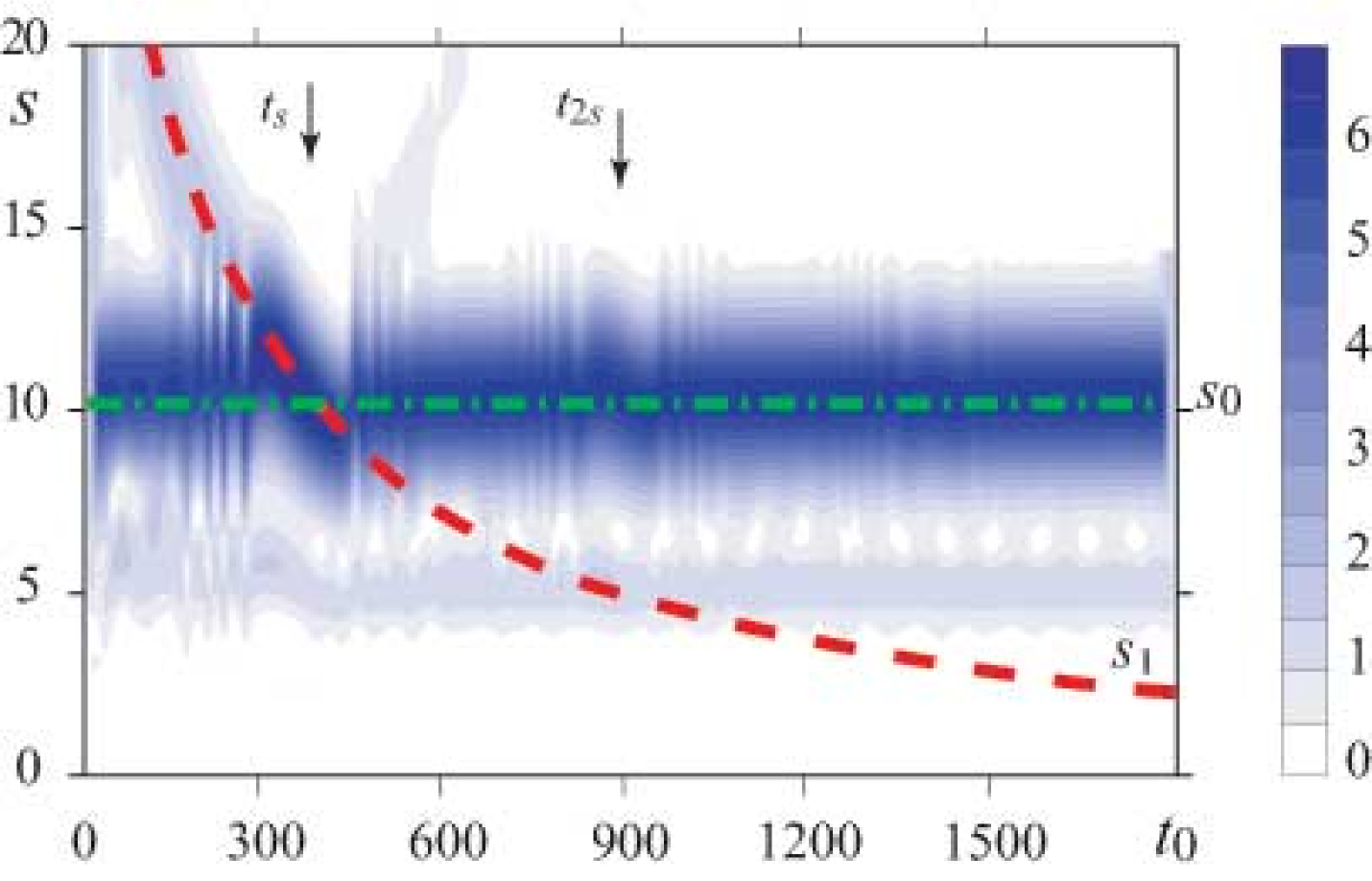
Fig. 1 shows the amplitude spectrum of the wavelet transform for the signal of driven oscillator (14). The Morlet wavelet is used as the mother wavelet function throughout the paper. The wavelet parameter is chosen to be , unless otherwise specified. The time scale corresponding to the first harmonic of the oscillator basic frequency is indicated in Fig. 1 by the dot-and-dash line. The dashed line indicates the time scale corresponding to the linearly increasing driving frequency . The analysis of the wavelet power spectrum reveals the classical picture of oscillator frequency locking by the external driving. As the result of this locking, the breaks appear close to the time moments and denoted by arrows, when the driving frequency is close to the oscillator basic frequency () or to its second harmonic (), respectively. These breaks represent the entrainment of oscillator frequency and its harmonic by external driving. If the detuning is great enough, the frequency of oscillations returns to the oscillator basic frequency.
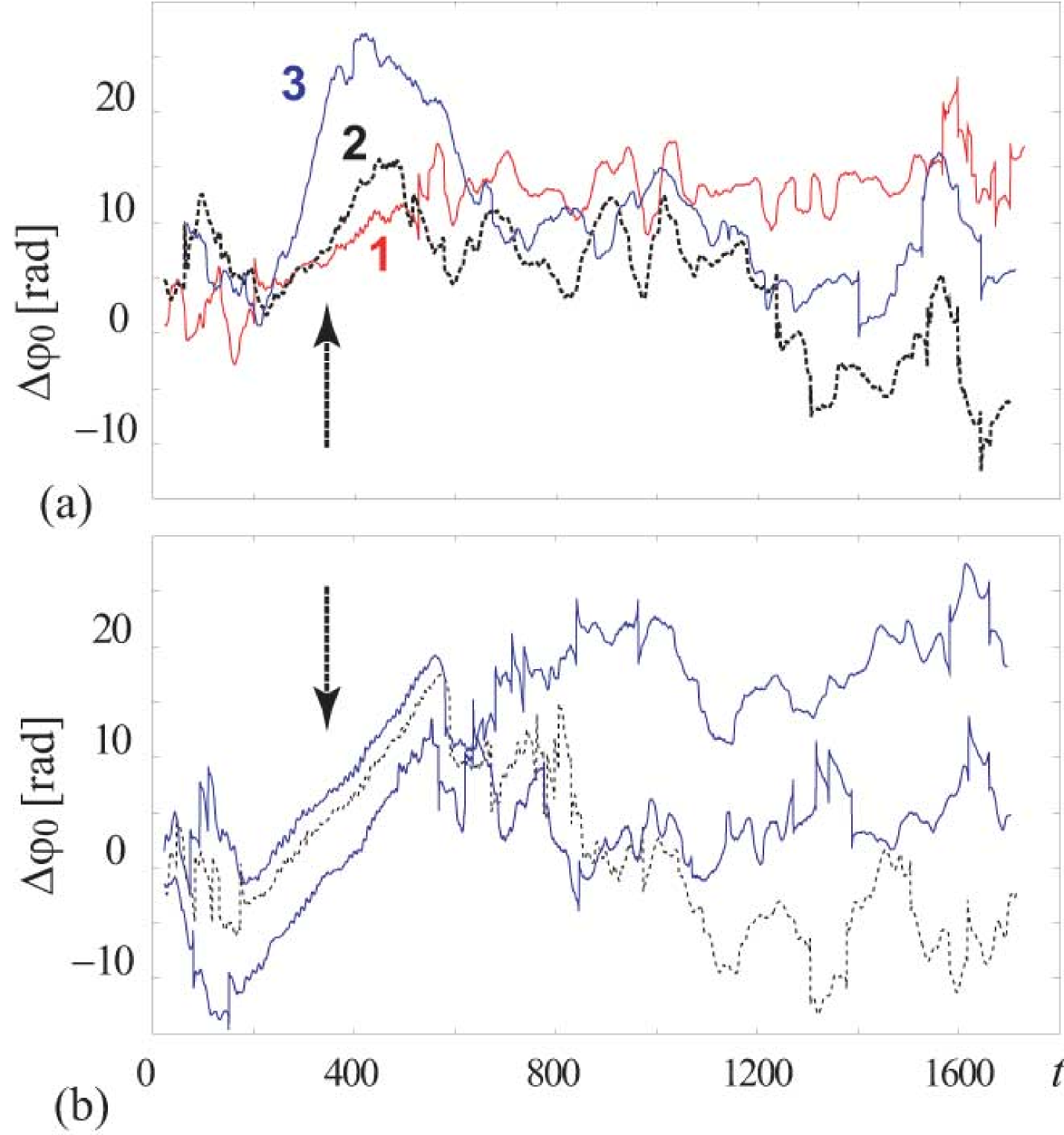
The dynamics of the phase differences determined by Eq. (3) is presented in Fig. 2a for different positive values. One can see in the figure the regions where is almost constant. These are the regions of asynchronous dynamics, when the driving frequency is far from the oscillator basic frequency and its harmonics. The regions of monotone increase of are also well-pronounced in Fig. 2a. These are the regions of synchronization observed in the vicinity of the time moments , when .
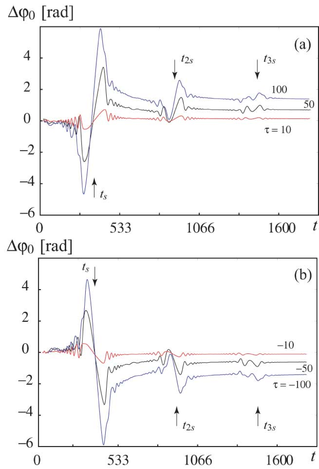
The proposed method offers several advantages over the method in Ref. Hramov A.E., Koronovskii A.A., Ponomarenko V.I., Prokhorov M.D. (2006) based on the analysis of the phase difference between the signals of oscillator and the external force. First, the regions of monotone variation corresponding to synchronous regimes are easily distinguished from the regions of constant value corresponding to asynchronous dynamics. Second, the new method is considerably more sensitive than the previous one because the phase difference is examined at the time scales having high amplitude in the wavelet spectrum. In particular, the region of synchronization in the vicinity of the time moment denoted by arrow is clearly identified in Fig. 2. Third, the proposed method is substantially simpler than the method of the phase difference calculation along the scale varying in time Hramov A.E., Koronovskii A.A., Ponomarenko V.I., Prokhorov M.D. (2006).
It follows from Eq. (7) that in the region of synchronization the change of the phase difference increases with increasing. As the result, the presence of interval of monotone variation becomes more pronounced, Fig. 2a. This feature helps to detect the existence of synchronization especially in the case of high-order synchronization and noise presence. However, the accuracy of determining the boundaries of the region of synchronization decreases as increases.
It should be noted that for negative values the monotone reduction of the phase difference is observed in the region of synchronization, Fig. 2b. As it can be seen from Fig. 2b, the increase of by absolute value leads to increase of variation in the region of synchronization as well as in the case of positive .
III.3 Influence of noise and inaccuracy of the basic time scale definition
Experimental data, especially those obtained from living systems, are always corrupted by noise. Besides, in many cases it is not possible to define accurately the basic frequency of the system under investigation. For example, interaction between the human cardiovascular and respiratory systems and nonstationarity hampers accurate estimation of natural frequencies for cardiovascular rhythms. Therefore, the actual problem is to test the method efficiency for detecting synchronization in the presence of additive noise and inaccuracy of the basic frequencies estimation.
To analyze the influence of noise on the diagnostics of synchronization we consider the signal
| (16) |
where is the signal of the asymmetric van der Pol oscillator (14), is the additive noise with zero mean and uniform distribution in the interval , and is the intensity of noise. To simulate the noisy signal we use the random-number generator described in Ref. Press W.H., Teukolsky S.A., Vetterling W.T., Flannery B.T. (1997).
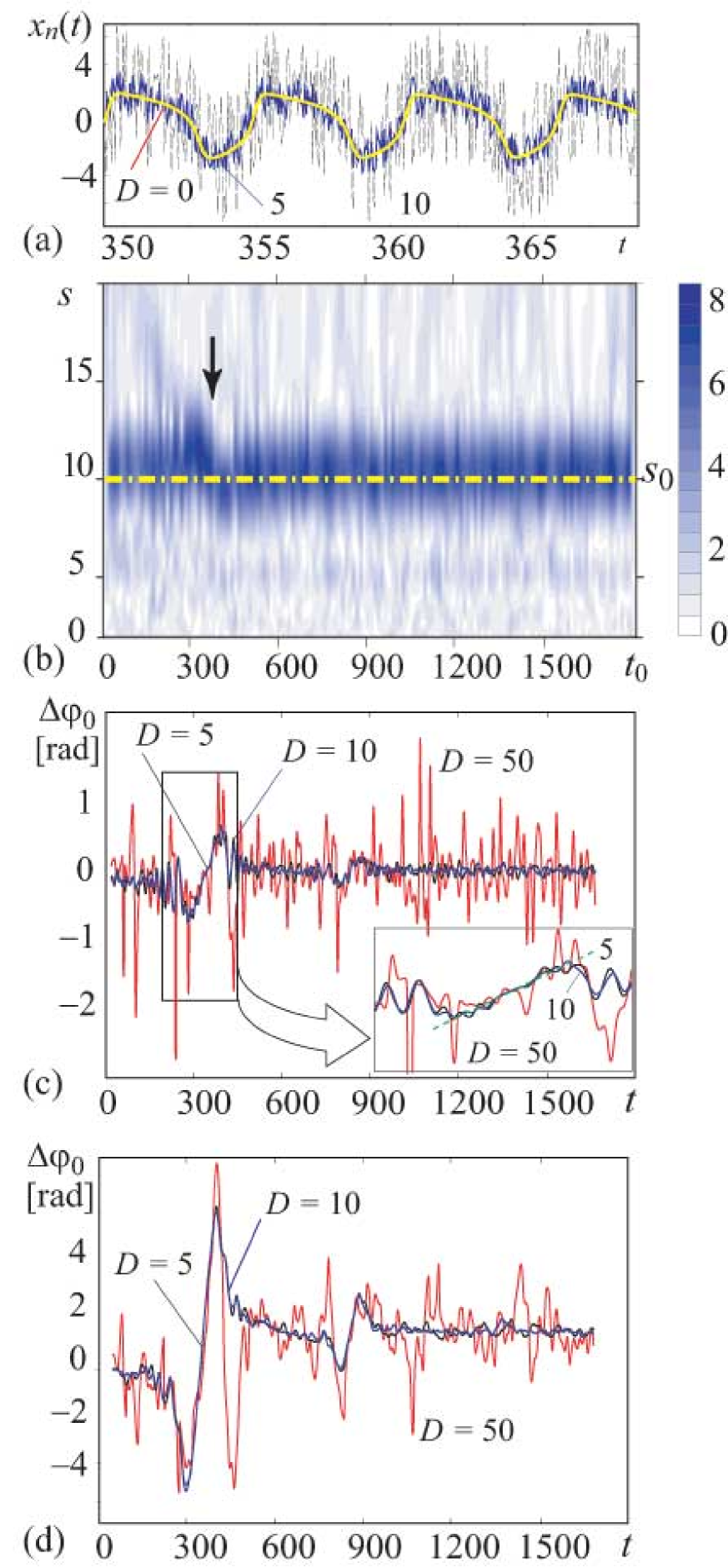
Typical time series generated by Eq. (16) for different intensities of noise are presented in Fig. 3a for the region of synchronization. In spite of the significant distortion of the signal by noise its wavelet power spectrum, Fig. 3b, still allows to reveal the main features of the system dynamics. In particular, the dynamics of the time scale and the effect of frequency entrainment in the region of synchronization indicated by arrow are recognized in Fig. 3b. Hence, the use of the wavelet transform for determining the phases of the signal and its harmonics allows one to detect the regimes of synchronization from noisy time series.
The phase differences calculated using Eq. (3) with are shown on Fig. 3c for different intensities of additive noise. The dependence becomes more jagged as increases. However, for we can identify the regions where the phase difference demonstrates near-monotone variation. In the average this variation is about the same as in the case of noise absence (see the inset in Fig. 3c). Fig. 3d shows for . In this case it is possible to detect the presence of synchronization for significantly higher levels of noise than in the case of small . The reason is that the value of (11) increases in the region of synchronization as the time shift increases, whereas the amplitude of fluctuations caused by noise does not depend on . For very large intensities of noise ( in Fig. 3) the synchronous behavior is not so clearly pronounced as at smaller values, but it should be mentioned that in this case the power of noise exceeds the power of the oscillator signal in several times.
Let us consider the method efficiency in the case when the scale of observation differs from the time scale associated with the oscillator basic frequency . Fig. 4 illustrates the behavior of the phase difference calculated for the time series of Eq. (16) at the time scales , where is the detuning of the scale with respect to the basic scale . It can be seen from the figure that for the phase dynamics is qualitatively similar to the case of accurate adjustment of the scale to the basic scale . At greater values the phase difference demonstrates significant fluctuations impeding to detect the epochs of monotone variation. Thus, to detect synchronization using the proposed method one needs to know only approximately the basic time scale .
IV Investigation of synchronization in a driven electronic oscillator with delayed feedback
IV.1 Experiment description
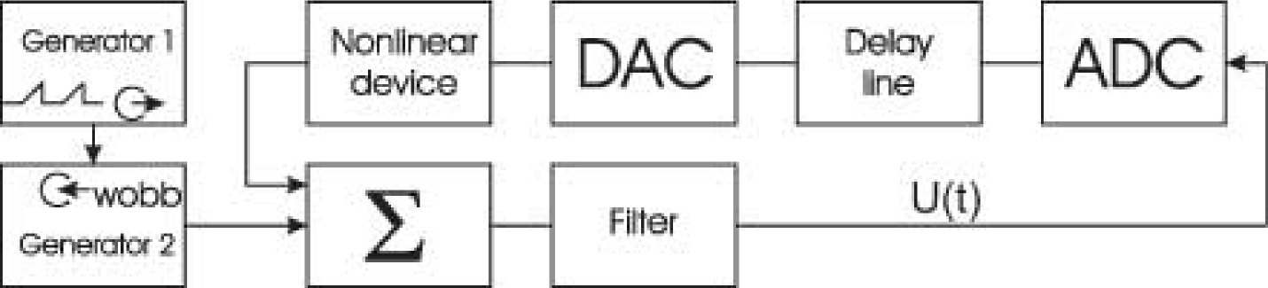
We apply the method to experimental data gained from a driven electronic oscillator with delayed feedback. A block diagram of the experimental setup is shown in Fig. 5. The oscillator represents the ring system composed of nonlinear, delay, and inertial elements. The role of nonlinear element is played by an amplifier with the quadratic transfer function. This nonlinear device is constructed using bipolar transistors. The delay line is constructed using digital elements. The inertial properties of the oscillator are defined by a low-frequency first-order -filter. The analogue and digital elements of the scheme are connected with the help of analog-to-digital (ADC) and digital-to-analog converters (DAC). To generate the driving signal we use the sine-wave generator 2 whose frequency is modulated through the wobble input by the signal of the sawtooth pulse generator 1. The driving signal is applied to the oscillator using the summator . The considered oscillator is governed by the first-order time-delay differential equation
| (17) |
where and are the delay line input and output voltages, respectively, is the delay time, and are the resistance and capacitance of the filter elements, is the transfer function of the nonlinear device, is the amplitude of the driving signal, and is the driving frequency. We record the signal using an analog-to-digital converter with the sampling frequency kHz at ms and ms under the following variation of the driving frequency
| (18) |
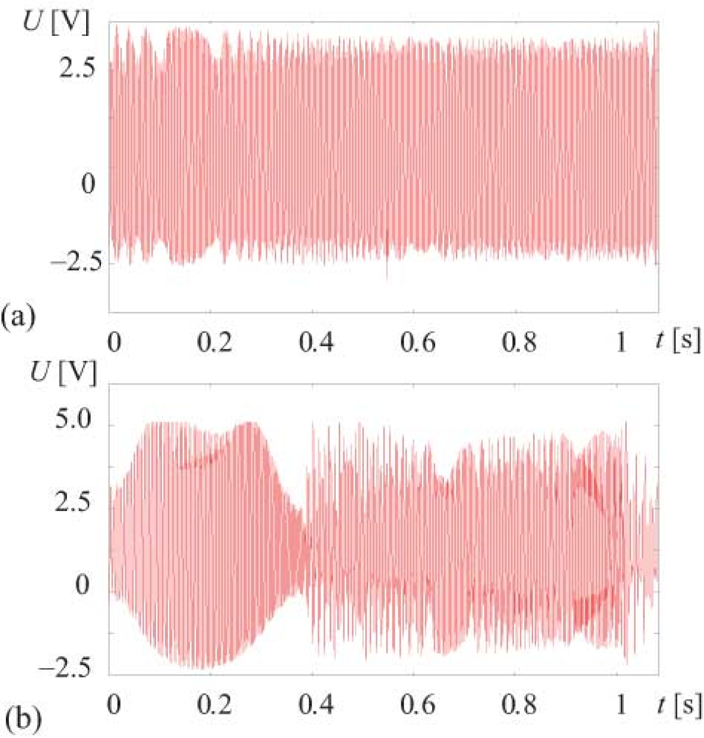
where Hz and the control voltage varies linearly from 0 V to 16 V within 800 ms providing variation from 220 Hz to 1000 Hz. Under the chosen parameters the considered oscillator demonstrates periodic oscillations with the period ms. Four experiments were carried out at different amplitudes of the external driving equal to 0.5 V, 1 V, 1.5 V, and 2 V. The amplitude of driven oscillation was about 3 V.
IV.2 Results
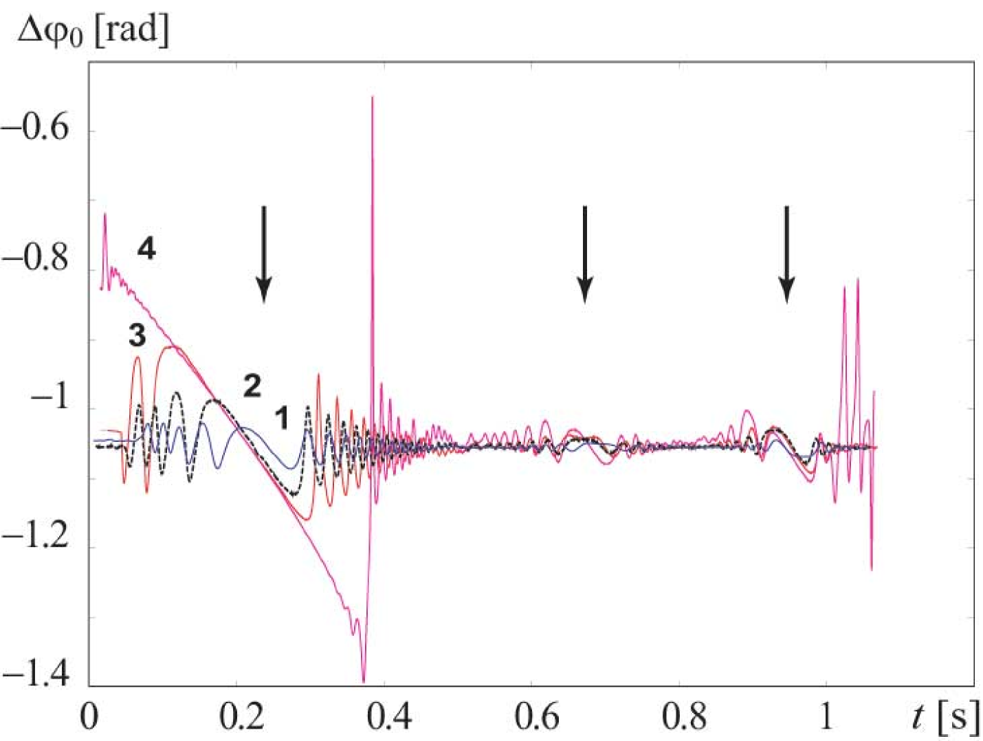
The experimental time series of the electronic oscillator with delayed feedback driven by the external force with varying frequency (18) are depicted in Fig. 6 for two values of the driving amplitude. The results of investigation of the oscillator synchronization by the external driving are presented in Fig. 7. The phase differences defined by Eq. (3) are calculated under different driving amplitudes for the time shift ms. One can clearly identify in the figure the regions of monotone variation corresponding to the closeness of the driving frequency to the oscillator basic frequency and its harmonics. These regions of synchronous dynamics are indicated by arrows.
It is well seen from Fig. 7 that the interval of monotone variation of increases with increasing amplitude of the driving force. This fact agrees well with the known effect of extension of the region of synchronization with increase in the amplitude of the external driving. Note, that in spite of the nonlinear variation of the driving frequency, at small driving amplitudes the phase difference varies almost linearly in time within the synchronization tongue as it was discussed in Sec. II. For the large driving amplitude ( V) the synchronization tongue is wide enough and the phase difference behavior begins to depart from linearity. Nevertheless, the variation of remains the monotone one and allows us to detect the presence of synchronization and estimate the boundaries of the synchronization tongue.
V Synchronization of slow oscillations in blood pressure by respiration from the data of heart rate variability
In this section we investigate synchronization between the respiration and rhythmic process of slow regulation of blood pressure and heart rate from the analysis of univariate data in the form of the heartbeat time series. This kind of synchronization has been experimentally studied in Prokhorov M.D., Ponomarenko V.I., Gridnev V.I., Bodrov M.B., Bespyatov A.B. (2003); Hramov A.E., Koronovskii A.A., Ponomarenko V.I., Prokhorov M.D. (2006); Janson:2001_PRL ; Janson:2002_PRE . We studied eight healthy volunteers. The signal of ECG was recorded with the sampling frequency 250 Hz and 16-bit resolution. Note, that according to Circulation:1996 the sampling frequency 250 Hz used in our experiments suffices to detect accurately the time moment of R peak appearance. The experiments were carried out under paced respiration with the breathing frequency linearly increasing from 0.05 Hz to 0.3 Hz within 30 min. We specially included the lower frequencies for paced respiration in order to illustrate the presence of the most pronounced regime of 1:1 synchronization between the respiration and slow oscillations in blood pressure. The rate of respiration was set by sound pulses. The detailed description of the experiment is given in Ref. Prokhorov M.D., Ponomarenko V.I., Gridnev V.I., Bodrov M.B., Bespyatov A.B. (2003).
Extracting from the ECG signal the sequence of R–R intervals, i.e., the series of the time intervals between the two successive R peaks, we obtain the information about the heart rate variability. The proposed method of detecting synchronization from uniform data was applied to the sequences of R–R intervals.
A typical time series of R–R intervals for breathing at linearly increasing frequency is shown in Fig. 8a. Since the sequence of R–R intervals is not equidistant, we exploit the technique for applying the continuous wavelet transform to nonequidistant data. The wavelet spectra for different parameters of the Morlet wavelet are shown in Figs. 8b and 8c for the sequence of R–R intervals presented in Fig. 8a. For greater values the wavelet transform provides higher resolution of frequency Koronovskii A.A., Hramov A.E. (2003) and better identification of the dynamics at the time scales corresponding to the basic frequency of oscillations and the varying respiratory frequency. In the case of the time scale of the wavelet transform is very close to the period of the Fourier transform and the values of are given in seconds in Fig. 8b. Generally, the time scale is related to the frequency of the Fourier transform by the following equation:
| (19) |
Because of this, the units on the ordinates are different in Figs. 8b and 8c. The wavelet spectra in these figures demonstrate the high-amplitude component corresponding to the varying respiratory frequency manifesting itself in the HRV data. The self-sustained slow oscillations in blood pressure (Mayer wave) have in humans the basic frequency of about 0.1 Hz, or respectively, the basic period close to 10 s. The power of this rhythm in the HRV data is less than the power of respiratory oscillations. As the result, the time scale is weakly pronounced in the spectra.
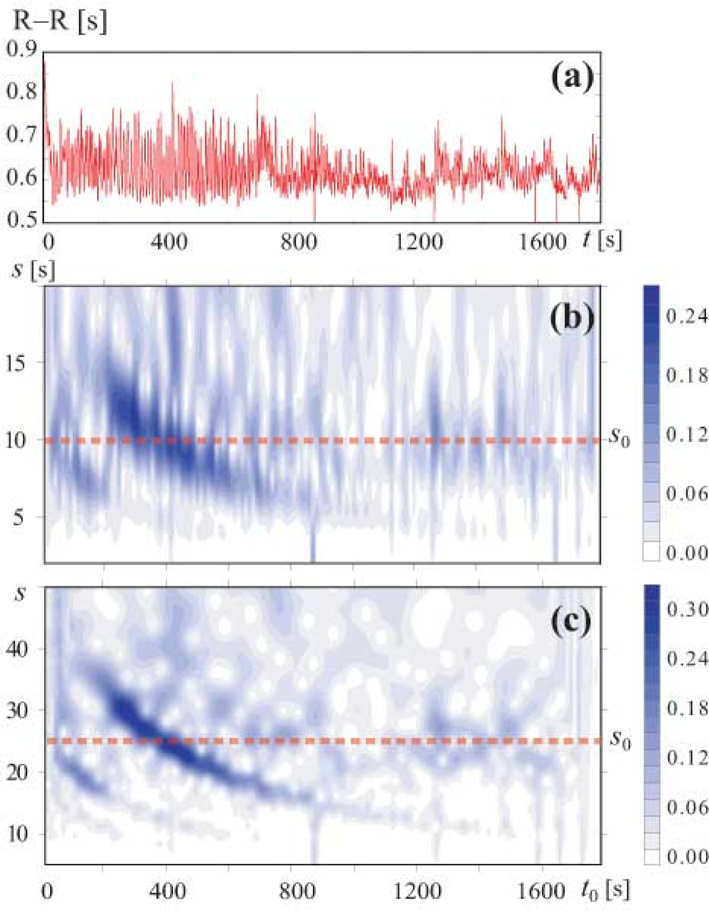
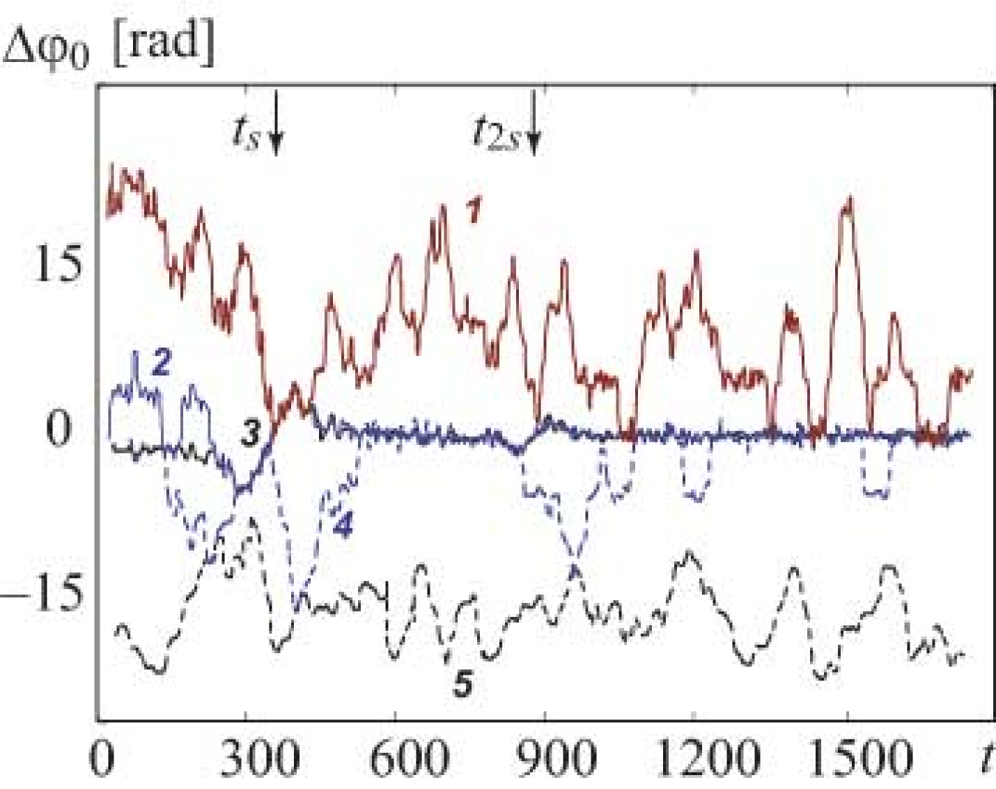
Fig. 9 presents the phase differences calculated for R–R intervals of four subjects under respiration with linearly increasing frequency. All the curves in the figure exhibit the regions with almost linear in the average variation of indicating the presence of synchronous dynamics. In particular, the region of synchronization is observed within the interval 200–600 s when the frequency of respiration is close to the basic frequency of the Mayer wave. This region is marked by arrow. In this region the frequency of blood pressure slow oscillations is locked by the increasing frequency of respiration and increases from 0.07 Hz to 0.14 Hz. Outside the interval of synchronization, s and s, the phase differences demonstrate fluctuations caused by the high level of noise and nonstationarity of the experimental data. Some of these fluctuations take place around an average value as well as in the case of the driven van der Pol oscillator affected by noise (see Fig. 3). The frequency of blood pressure slow oscillations demonstrates small fluctuations around the mean value of about 0.1 Hz outside the interval of synchronization.
The phase differences in Fig. 9a are plotted for different . As the time shift increases, so does the range of monotone variation in the region of synchronization. This result agrees well with the results presented in Sec. III. Similar behavior of is observed for each of the eight subjects studied. In Fig. 9(b) phase differences computed for R-R intervals of another three subjects are presented. The phase differences demonstrate the wide regions of almost linear variation for all the subjects. Such behavior of the considered phase difference cannot be observed in the absence of synchronization, if only the modulation of blood pressure oscillations by respiration is present. These results allow us to confirm the conclusion that the slow oscillations in blood pressure can be synchronized by respiration. However, to come to this conclusion, the proposed method needs only univariate data in distinction to the methods Prokhorov M.D., Ponomarenko V.I., Gridnev V.I., Bodrov M.B., Bespyatov A.B. (2003); Hramov A.E., Koronovskii A.A., Ponomarenko V.I., Prokhorov M.D. (2006) based on the analysis of bivariate data. Note, that paper Prokhorov M.D., Ponomarenko V.I., Gridnev V.I., Bodrov M.B., Bespyatov A.B. (2003) contains the more detailed investigation of synchronization between the respiration and slow oscillations in blood pressure than the present one. Recent reports (see, for examples, Rosenblum:1998_Nature ; Suder:1998_AJP ; Kotani:2000_MIM ) focused on examining the relationship between respiration and heart rate have shown that there is nonlinear coupling between respiration and heart rate. In particular, such coupling is well studied for the respiratory modulation of heart rate Bishop:1981_AJP ; Kotani:2000_MIM known as respiratory sinus arrhythmia. The presence of coupling between the cardiac and respiratory oscillatory processes has been revealed also using bispectral analysis in Jamsek:2003_PRE ; Jamsek:2004_PMB under both spontaneous and paced respiration. Our results are in agreement with those when synchronization between the oscillating processes occurs as the result of their interaction.
VI Conclusion
We have proposed the method for detecting synchronization from univariate data. The method allows one to detect the presence of synchronization of the self-sustained oscillator by external force with varying frequency. To implement the method one needs to analyze the difference between the oscillator instantaneous phases calculated at time moments shifted by a certain constant value with respect to each other. The instantaneous phases are defined at the oscillator basic frequency using continuous wavelet transform with the Morlet wavelet as the mother wavelet function. The necessary condition for the method application is the variation of the frequency of the driving signal. The method efficiency is illustrated using both numerical and experimental univariate data under sufficiently high levels of noise and inaccuracy of the basic time scale definition.
We applied the proposed method to studying synchronization between the respiration and slow oscillations in blood pressure from univariate data in the form of R–R intervals. The presence of synchronization between these rhythmic processes is demonstrated within the wide time interval. The knowledge about synchronization between the rhythms of the cardiovascular system under paced respiration is useful for the diagnostics of its state N. Ancona, R. Maestri, D. Marinazzo, L. Nitti, M. Pellicoro, G.D. Pinna, S. Stramaglia (2005). The method allows one to detect the presence of synchronization from the analysis of the data of Holter monitor widely used in cardiology.
The proposed method can be used for the analysis of synchronization even in the case when the law of the driving frequency variation is unknown. If the frequency of the external driving varies in the wide range, the analysis of the oscillator response to the unknown driving force allows one to make a conclusion about the presence or absence of synchronization in the system under investigation.
Acknowledgments
We thank Dr. Svetlana Eremina for English language support. This work is supported by the Russian Foundation for Basic Research, Grants 05–02–16273, 07–02–00044, 07–02–00747 and 07–02–00589, and the President Program for support of the leading scientific schools in the Russian Federation, Grant No. SCH-4167.2006.2. A.E.H. acknowledges support from CRDF, Grant No. Y2–P–06–06. A.E.H. and A.A.K. thank the “Dynasty” Foundation for the financial support.
References
- Blekhman I.I. (1971) Blekhman I.I., Synchronization of dynamical systems (Moscow, Nauka, 1971).
- Blekhman I.I. (1988) Blekhman I.I., Synchronization in Science and Technology (American Society of Mechanical Engineers, 1988).
- Pikovsky A., Rosenblum M., Kurths J. (2001) Pikovsky A., Rosenblum M., Kurths J., Synhronization: a universal concept in nonlinear sciences (Cambridge University Press, Cambridge, 2001).
- Boccaletti S., Kurths J., Osipov G., Valladares D.L., Zhou C. (2002) Boccaletti S., Kurths J., Osipov G., Valladares D.L., Zhou C., Physics Reports 366, 1 (2002).
- Rosenblum M., Pikovsky A., Kurths J., Schafer C., Tass P. (2001) Rosenblum M., Pikovsky A., Kurths J., Schafer C., Tass P., in Handbook of Biological Physics (Elsiver Science, 2001), pp. 279–321.
- Meinecke F.C., Ziehe A., Kurths J., Müller K.-R. (2005) Meinecke F.C., Ziehe A., Kurths J., Müller K.-R., Phys. Rev. Lett. 94, 084102 (2005).
- Hramov A.E., Koronovskii A.A. (2004) Hramov A.E., Koronovskii A.A., Chaos 14, 603 (2004).
- Hramov A.E., Koronovskii A.A., Kurovskaya M.K., Moskalenko O.I. (2005) Hramov A.E., Koronovskii A.A., Kurovskaya M.K., Moskalenko O.I., Phys. Rev. E 71, 056204 (2005).
- Pecora L.M., Carroll T.L. (1990) Pecora L.M., Carroll T.L., Phys. Rev. Lett. 64, 821 (1990).
- Pecora L.M., Carroll T.L., Jonson G.A., Mar D.J. (1997) Pecora L.M., Carroll T.L., Jonson G.A., Mar D.J., Chaos 7, 520 (1997).
- Pikovsky A., Rosenblum M., Kurths J. (2000) Pikovsky A., Rosenblum M., Kurths J., Int. J. Bifurcation and Chaos 10, 2291 (2000).
- Boccaletti S., Pecora L.M., Pelaez A. (2001) Boccaletti S., Pecora L.M., Pelaez A., Phys. Rev. E 63, 066219 (2001).
- Rulkov N.F., Sushchik M.M., Tsimring L.S., Abarbanel H.D.I. (1995) Rulkov N.F., Sushchik M.M., Tsimring L.S., Abarbanel H.D.I., Phys. Rev. E 51, 980 (1995).
- Pyragas K. (1996) Pyragas K., Phys. Rev. E 54, R4508 (1996).
- Tass et al. (1998) P. Tass, M. G. Rosenblum, J. Weule, J. Kurths, A. Pikovsky, J. Volkmann, A. Schnitzler, and H.-J. Freund, Phys. Rev. Lett. 81, 3291 (1998).
- Tass et al. (2003) P. A. Tass, T. Fieseler, J. Dammers, K. Dolan, P. Morosan, M. Majtanik, F. Boers, A. Muren, K. Zilles, and G. R. Fink, Phys. Rev. Lett. 90, 088101 (2003).
- Chavez M., Adam C., Navarro, Boccaletti S., Martinerie J. (2005) Chavez M., Adam C., Navarro, Boccaletti S., Martinerie J., Chaos 15 (2005).
- Schäfer C., Rosenblum M.G., Abel H.-H., Kurths J. (1999) Schäfer C., Rosenblum M.G., Abel H.-H., Kurths J., Phys. Rev. E 60, 857 (1999).
- Bračič-Lotrič M., Stefanovska A. (2000) Bračič-Lotrič M., Stefanovska A., Physica A 283, 451 (2000).
- Rzeczinski S., Janson N.B., Balanov A.G., McClintock P.V.E. (2002) Rzeczinski S., Janson N.B., Balanov A.G., McClintock P.V.E., Phys. Rev. E 66, 051909 (2002).
- Prokhorov M.D., Ponomarenko V.I., Gridnev V.I., Bodrov M.B., Bespyatov A.B. (2003) Prokhorov M.D., Ponomarenko V.I., Gridnev V.I., Bodrov M.B., Bespyatov A.B., Phys. Rev. E 68, 041913 (2003).
- Hramov A.E., Koronovskii A.A., Ponomarenko V.I., Prokhorov M.D. (2006) Hramov A.E., Koronovskii A.A., Ponomarenko V.I., Prokhorov M.D., Phys. Rev. E 73, 026208 (2006).
- Hramov A.E., Koronovskii A.A., Levin Yu.I (2005) Hramov A.E., Koronovskii A.A., Levin Yu.I, JETP 127, 886 (2005).
- Hramov A.E., Koronovskii A.A. (2005) Hramov A.E., Koronovskii A.A., Physica D 206, 252 (2005).
- Hramov A.E., Koronovskii A.A., Popov P.V., Rempen I.S. (2005) Hramov A.E., Koronovskii A.A., Popov P.V., Rempen I.S., Chaos 15, 013705 (2005).
- Malpas S. (2002) Malpas S., Am. J. Physiol. Heart Circ. Physiol. 282, H6 (2002).
- Stefanovska A., Hožič M. (2000) Stefanovska A., Hožič M., Prog. Theor. Phys. Suppl. 139, 270 (2000).
- Adler R. (1947) Adler R., Proc. IRE 35, 1415–1423 (1947).
- Koronovskii A.A., Hramov A.E. (2004) Koronovskii A.A., Hramov A.E., JETP Lett. 79, 316 (2004).
- Wav (2004) Wavelets in Physics (Cambridge University Press, Cambridge, 2004), J.C. Van den Berg ed.
- Koronovskii A.A., Hramov A.E. (2003) Koronovskii A.A., Hramov A.E., Continuous wavelet analysis and its applications (Moscow, Fizmatlit, 2003).
- (32) Lachaux J.P., Rodriguez E., Martinerie J., Varela F.J., Human Brain Mapping 8, 194, (1999).
- (33) Lachaux J.P., Rodriguez E., Van Quyen M.L., Lutz A., Martinerie J., Varela F.J., Int. J. Bifurcation and Chaos. 10, 2429 (2000).
- (34) Le Van Quyen M., Foucher J., Lachaux J.P., Rodriguez E., Lutz A., Martinerie J., Varela F.J. J. Neuroscience Methods 111, 83 (2001).
- (35) Lachaux J.P., Lutz A., Rudrauf D., Cosmelli D., Le Van Quyen M., Martinerie J., Varela F. Neurophysiol. Clin., 32, 157 (2002).
- (36) Quyen M. L., Foucher J., Lachaux J.-P., Rodriguez E., Lutz A., Martinerie J., Varela F. J. J. Neuroscience Methods 111, 83 (2001).
- (37) Quiroga R.Q., Kraskov A., Kreuz T., Grassberger P. Phys. Rev. E 65, 041903 (2002).
- (38) Turalska M., Kolodziej W., Latka M., Latka D., West B.J. Shock 23, Suppl. 3, 90 (2005).
- (39) DeShazer D. J., Breban R., Ott E., and Roy R. Phys. Rev. Lett. 87, 044101 (2001).
- (40) Sosnovtseva O. V., Pavlov A. N., Mosekilde E., and Holstein-Rathlou N.-H. Phys. Rev. E 66, 061909 (2002).
- (41) Bandrivskyy A., Bernjak A., McClintock P. V. E., and Stefanovska A. Cardiovasc. Eng. Int. J. 4, 89 (2004).
- Grossman A. and Morlet J. (1984) Grossman A. and Morlet J., SIAM J. Math. Anal. 15, 273 (1984).
- Press W.H., Teukolsky S.A., Vetterling W.T., Flannery B.T. (1997) Press W.H., Teukolsky S.A., Vetterling W.T., Flannery B.T., Numerical Recipes (Cambridge University Press, Cambridge, 1997).
- (44) Janson N. B., Balanov A. G., Anishchenko V. S., McClintock P. V. E. Phys. Rev. E 86, 1749 (2001).
- (45) Janson N. B., Balanov A. G., Anishchenko V. S., McClintock P. V. E. Phys. Rev. E 65, 036212 (2002).
- (46) Task Force of the ESC and NASPE, Circulation 93, 1043, (1996).
- (47) Shäfer C., Rosenblum M.G., Abel H.H. Nature 392, 239 (1998).
- (48) Suder K., Drepper F.R., Schiek M., Abel H.H. Am. J. Physiol. 275, H33 (1998).
- (49) Hirsch J.A., Bishop B. Am. J. Physiol. 241, H620 (1981).
- (50) Kotani K., Hidaka I., Yamamoto Y., Ozono S. Method Inform Med. 39, 153 (2000).
- (51) Jamšek J., Stefanovska A., McClintock P.V.E., Khovanov I.A. Phys. Rev. E 68, 016201 (2003).
- (52) Jamšek J., Stefanovska A., McClintock P.V.E. Phys. Med. Biol. 49, 4407 (2004).
- N. Ancona, R. Maestri, D. Marinazzo, L. Nitti, M. Pellicoro, G.D. Pinna, S. Stramaglia (2005) N. Ancona, R. Maestri, D. Marinazzo, L. Nitti, M. Pellicoro, G.D. Pinna, S. Stramaglia, Physiological Measurement 26, 363–372 (2005).