Determining Model-Independent and Consistency Tests
Abstract
We determine the Hubble constant precisely (2.3% uncertainty) in a manner independent of cosmological model through Gaussian process regression, using strong lensing and supernova data. Strong gravitational lensing of a variable source can provide a time-delay distance and angular diameter distance to the lens . These absolute distances can anchor Type Ia supernovae, which give an excellent constraint on the shape of the distance-redshift relation. Updating our previous results to use the H0LiCOW program’s milestone dataset consisting of six lenses, four of which have both and measurements, we obtain for a flat universe and for a non-flat universe. We carry out several consistency checks on the data and find no statistically significant tensions, though a noticeable redshift dependence persists in a particular systematic manner that we investigate. Speculating on the possibility that this trend of derived Hubble constant with lens distance is physical, we show how this can arise through modified gravity light propagation, which would also impact the weak lensing tension.
Subject headings:
cosmology: cosmological parameters - distance scale - gravitational lensing: strong1. Introduction
The flat cosmological constant plus cold dark matter (CDM) model is currently taken as the concordance cosmological scenario and explains a wide range of observations. However, there is significant tension in the value inferred within CDM from the cosmic microwave background (CMB) observations (Planck, 2018) and that measured through the Cepheid distance ladder, (Riess et al., 2019). Other cosmological probes such as baryon acoustic oscillations together with primordial nucleosynthesis constraints agree with the CMB value of (Addison et al., 2018; Macaulay et al., 2019; Cuceu et al., 2019; Philcox et al., 2020), while other distance ladder techniques can lie in between (Freedman et al., 2020).
The discrepancy could arise due to unaccounted for systematic errors in observations or reveal new physics significantly different from CDM.
Independent cosmological probes could provide new perspectives. Strong gravitational lensing by galaxies offers an independent method of determining through time-delay lens systems. A typical lensing system consists of a distant active galactic nucleus (AGN) lensed by a foreground elliptical galaxy, forming multiple images along with the arcs of the host galaxy. The images will be magnified and the light will arrive at the Earth delayed by various times. Since AGNs are variable, we can measure the time delays between any two images from their light curves.
From the time delay plus the lens potential measured by the high-resolution imaging and line-of-sight environment we can measure the “time-delay distance” . This is a combination of three angular diameter distances, primarily depending on though also more weakly depending on the cosmological model, e.g. the matter density, dark energy properties, etc. In addition, with kinematic information on the lens galaxy (for example the velocity dispersion) the angular diameter distance to the lens can be also determined independent of the external convergence from line of sight perturbers (Paraficz & Hjorth, 2009; Jee et al., 2015, 2016).
Either or , or both jointly, provides a one-step method of determining , which is substantially independent of and complementary to the CMB, large scale structure, and distance ladder methods. Thus they give a much needed crosscheck. However, like the other cosmological probes, one has to assign a cosmological model when computing the lensing distances. The results may therefore differ for different models.
Rather than computing the distances within a model, one can instead measure the distance-redshift relation. To do so, one needs a probe that is both accurate and samples distance much more densely. Type Ia supernovae (SNe Ia) are superb mappers of the distance-redshift relation. However, they only provide relative distances because the SNe absolute magnitude (and Hubble constant) is unknown. The strengths of the two probes can combine together to remove each weakness: absolute distance measurements from time-delay lensing and relative distances from SNe Ia can anchor each other (for anchoring one type of distance with another, see for example Aubourg et al. (2015); Cuesta et al. (2015); Collett et al. (2019); Pandey, Raveri, Jain (2019)). When combining the two, the results under different cosmological models seem to be stable and consistent (Taubenberger et al., 2019).
One can make the cosmology-model independence (i.e. no form assumed for the expansion history ) more explicit than simply checking under different models. In Liao et al. (2019) we applied Gaussian process (GP) regression to SNe Ia data to get a model-independent relative distance-redshift relation, i.e. the shape of distance-redshift function. Anchoring this together with from 4 H0LiCOW lenses resulted in in a flat universe and considering the cosmic curvature density in the range .
Currently, the H0LiCOW program has reached its first milestone (Wong et al., 2019). The full dataset consists of 6 lenses, five of which were analyzed blindly, and four of which have both and measurements. In a flat CDM cosmology, they found , consistent with the local Cepheid distance ladder measurement but in tension with and other CMB and large scale structure measurements. Note the H0LiCOW results vary with the assumed models (Wong et al., 2019), although tends to increase with the usual generalized cosmologies. Furthermore, the previously identified trend (Wong et al., 2019; Liao et al., 2019) in derived value, or time delay distance excess, with redshift persists. Therefore, it is timely and useful to update our model-independent results.
We briefly introduce the H0LiCOW program and the lensing dataset in Section 2, and present our methodology and updated results in Section 3. In Section 4 we carry out some consistency checks between lensing data, and between lensing and supernova data. We explore the previously identified trend of with time-delay distance or lens redshift in Section 5, and present a possible physical explanation based on modified gravity. We summarize and discuss the results and next steps in Section 6.
2. Lensing distances and H0LiCOW program
Strong lensing (SL) by elliptical galaxies is a powerful tool to study both astrophysics and cosmology (Treu, 2010). Lenses with time-delay measurements were proposed to measure (Refsdal, 1964; Treu & Marshall, 2016). Specifically, the time delay between any two images is determined by
| (1) |
where the time-delay distance
| (2) |
is a combination of three angular diameter distances , where the subscripts d and s denote the deflector (lens) and the source, respectively. We use units where throughout the article. The Fermat potential difference between the two images is a function of lens mass profile parameters , determined by high-resolution imaging of the host arcs. Note that all other mass along the line of sight could also contribute to the lens potential, causing additional (de)focusing of the light rays and affecting the observed time delays. Considering the effects of the perturber masses are small, they can be approximated by an external convergence . Then the inferred will be scaled by 1-. Independent observations such as galaxy counts could break the degenaracy (Rusu et al., 2017). We take the time delay distances as given by H0LiCOW, and refer readers to the systematics treatment in Millon et al. (2019).
Additional information on the lens galaxy such as the light profile , the projected stellar velocity dispersion , and the anisotropy distribution of the stellar orbits, parametrized by , can yield the angular diameter distance to the lens (Birrer et al., 2016, 2019):
| (3) |
which correlates with . The function captures all the model components computed from angles measured on the sky (from imaging) and the stellar orbital anisotropy distribution (from spectroscopy). We refer to Section 4.6 of Birrer et al. (2019) for the detailed modeling related to .
The state-of-the-art lensing collaboration H0LiCOW aims at measuring with precision using time-delay lenses (Suyu et al., 2017). They take advantage of substantial data consisting of time-delay measurements from the COSMOGRAIL program111http://www.cosmograil.org and radio-wavelength monitoring, deep HST and ground-based adaptive optics imaging, spectroscopy of the lens galaxy, and deep wide-field spectroscopy and imaging.
In the recent milestone paper (Wong et al., 2019), they gave the latest constraints on under different cosmological models with a combined sample of six lenses that span a range of lens and source redshifts, as well as various image configurations (double, cross, fold, and cusp). All lenses except the earliest, B1608+656, were analyzed blindly with respect to the cosmological parameters. Four lenses (RXJ1131-1231, PG 1115+080, B1608+656, SDSS 1206+4332) have both and measurements. Note that and measurements for a system are correlated except for B1608+656 whose distance measurements are independent. The distance posterior distributions are released in the form of MCMC chains or skewed log-normal function fits on the H0LiCOW website222http://www.h0licow.org. For the case of MCMC chains, we will get the likelihood functions by smoothing the discrete points. We summarize the redshifts and measured distances in Table 1 ordered by the lens redshift. For more detailed information on these lenses, see Wong et al. (2019) and the references therein.
| Order | Name | (Mpc) | (Mpc) | references | ||
|---|---|---|---|---|---|---|
| 1 | RXJ1131-1231 | 0.295 | 0.654 | (1)(2) | ||
| 2 | PG 1115+080 | 0.311 | 1.722 | (1) | ||
| 3 | HE 0435-1223 | 0.4546 | 1.693 | - | (1)(3) | |
| 4 | B1608+656 | 0.6304 | 1.394 | (4)(5) | ||
| 5 | WFI2033-4723 | 0.6575 | 1.662 | - | (6) | |
| 6 | SDSS 1206+4332 | 0.745 | 1.789 | (7) |
3. Methodology and results
To combine the SNe data with lensing data, we generate samples of unanchored luminosity distance from the posterior of the Pantheon compilation from Scolnic et al. (2018), calculated with a GP (See, e.g., Koo et al. (2020) for a test of cosmology model independence.) This paper follows the analysis in Liao et al. (2019), which is based on the gphist (Kirkby & Keeley, 2017) code first presented in Joudaki et al. (2018).
Regression using a GP works by generating a set of functions from an infinite dimensional function space characterized by a covariance function. This covariance function is parametrized by a squared-exponential kernel
| (4) |
where and is the maximum redshift of the supernova sample. This has two hyper-parameters that are marginalized over, and , with determining the amplitude of the random fluctuations and determining the coherence length of the fluctuation, equivalently is proportional to the number of fluctuations in the range. The priors on these hyper-parameters are scale-invariant and we directly integrate over this space since the dimensionality is small.
The GP function involves the expansion history (which can be integrated to give distances), and is the best-fit CDM expansion history from the Pantheon dataset and works as the mean function of the GP regression. The GP prior functions are then trained on the Pantheon likelihood, which constrains only the shape of the expansion history, not the absolute scale, so unanchored luminosity distances are the quantities most directly constrained by the Pantheon SNe dataset.
| Case | (Liao et al. 2019) | (non-flat) | |||
|---|---|---|---|---|---|
| () |
| Lens | RXJ1131-1231 | PG 1115+80 | HE0435-1223 | B1608+656 | WFI2033-4723 | SDSS 1206+4332 |
|---|---|---|---|---|---|---|
| () |
To summarize the method for determining :
-
1.
Draw 1000 unanchored luminosity distance curves from the GP fit to the SNe data, and convert to unanchored angular diameter distances ;
-
2.
Evaluate the values of each of the 1000 curves at the lens and source redshifts of the six (SL) systems to calculate 1000 values of for each system using
(5) -
3.
Compute the likelihood, for each of the 1000 realizations, from the H0LiCOW’s combined with data (if the measurements are available) for each lens system for many values of ;
-
4.
Multiply the six likelihoods to form the full likelihood for each realization, for each value of ;
-
5.
Marginalize over the realizations to form the posterior distribution of .
Note that to obtain the angular diameter distance between the lens and the source from in step 2, we use the standard distance relation (Weinberg, 1972)
| (6) |
where is the dimensionless curvature density. For a spatially flat universe, one simply has .
In step 3, we also evaluate a case with the SL data alone. In such a case, the anchoring is direct between absolute and relative distances and one does not need to consider the assumption of cosmic curvature.
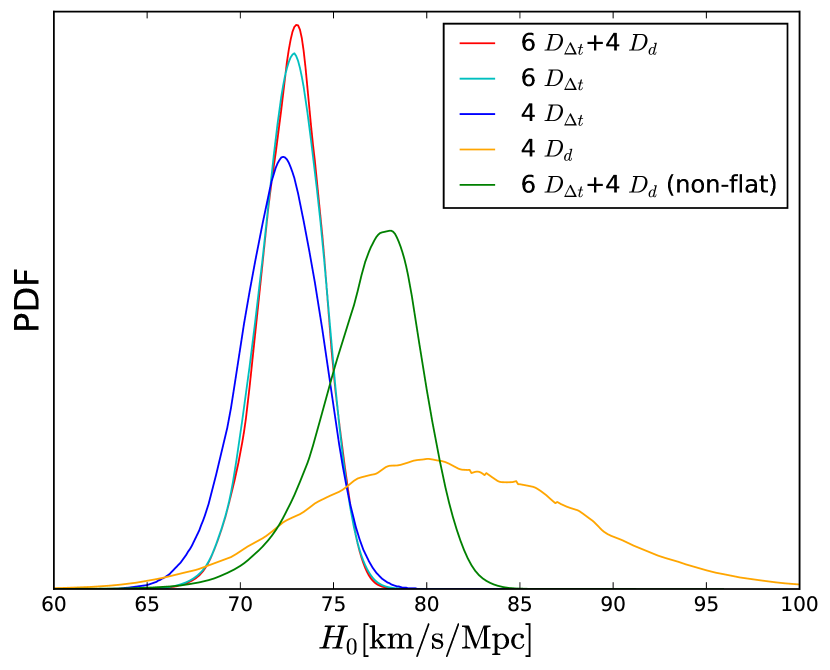
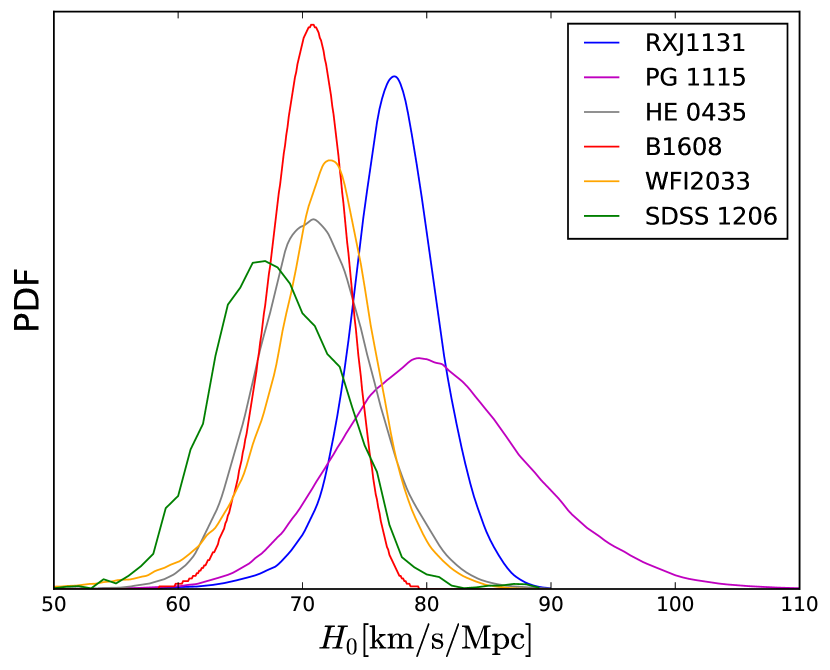
Figure 1 shows the joint posteriors and the numerical results are summarized in Table 2. First of all, we consider the full data set consisting of 6 lenses, 4 of which have both and measurements. The constraint is assuming the universe is flat. It is more stringent than our previous result based on 4 lenses with only data, . This model-independent result has comparable value and error bars as that under the flat CDM model by H0LiCOW, , supporting the tension with the BAO and CMB results. (Note that the looser constraints expected from removing the CDM assumption are offset by including supernova distances.)
In addition, we test the contribution of the data by taking and separately. The constraint from 4 data alone is relatively weaker, , and the 6 data show almost the same constraint power, , as the full set. Nevertheless, the result from data is free from assumptions concerning spatial curvature (although note that other lens parameters, such as stellar anisotropy, enter.)
We also consider the non-flat case for the full dataset for completeness. We set the uniform prior of the curvature parameter to be as in Wong et al. (2019). The constraints are and . Like the CDM-assumed case where , (Wong et al., 2019), our non-flat result shows a larger (possibly the data, which give a higher , have more influence in this case) and slightly favors an open universe. However, the change of relative to the flat case in this work is more distinct. It is worth mentioning that the constraint on in our method is model-independent as well.
Furthermore, to understand the relative contributions, we constrain with each lens in the model-independent manner. We use both and data (if it has). Figure 2 shows the individual posteriors. The numerical results are shown in Table 3, in order of increasing lens redshift. As one can see, a trend may exist: the values roughly decrease with the lens redshift or the distance. Our results further confirm the trend noticed in Wong et al. (2019); Liao et al. (2019) and shown in Fig. 5 in Millon et al. (2019) based on CDM. We explore this further in Section 5.
4. Consistency tests
In this section, we check to what extent the SL data are internally consistent and to what extent they are consistent with the SNe data. This is important to confirm that the results from the combination of lens systems, and from combination of SL and SNe, are robust. As the available SL distances become more numerous and more precise, one can better assess the consistency of these distances with the SNe distances. We begin by comparing the distance posteriors of the SL data, with the values of those quantities predicted by the SNe data.
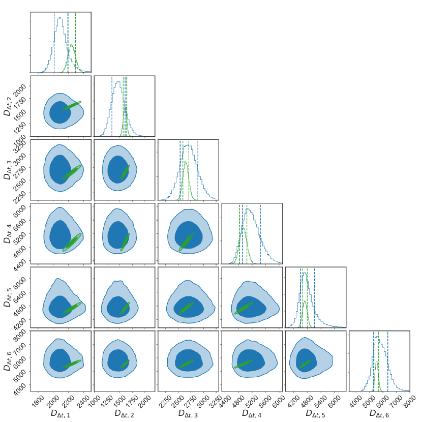
In Fig. 3, we plot the measured posteriors of the individual systems’ time-delay distances at the 68% and 95% confidence level, as well as the SNe posterior predictions of those systems’ time-delay distances using a GP regression on the Pantheon data. (The uncertainties on the angular distances are currently too large to add useful information to this comparison.) Since the SNe cannot constrain an absolute scale, the SNe posterior predictions for the SL distances are anchored in this figure by our combined measurement , giving the extended green contours, reflecting both the uncertainty in and the GP-based unanchored distances (). On the whole, the measurements of the SL distances are consistent with the SNe posterior predictions, in both the 1D and 2D joint posteriors, although since we have ordered the systems by lens redshift one can notice a tendency for the SL posterior to drift rightward (to higher distance and hence lower ) across the SNe posterior with increasing redshift. This will be explored further in Sec. 5.
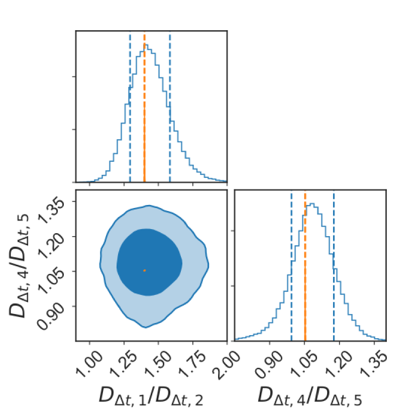
By forming ratios of time-delay distances, we can cancel out the dependence on , forming relative distances that the SNe are particularly suited to. In Fig. 4, we plot the measured SL posteriors of the ratios of time-delay distances for certain combinations of the systems, as well as the posterior predictions for those ratios from the SNe data. Indeed, the SNe posterior predictions are nearly pointlike. Rather than showing hundreds of 2D joint combinations of the 15 possible time-delay ratios, we select two cases: the left panel shows the ratios for the two pairs of systems nearly at the same lens redshift (see Table 1), and the right panel for two pairs of systems with the most extreme differences in lens redshift. The pairs nearly at the same redshift (one pair with both and one pair with both ) are highly consistent with the very precise SNe predictions. Those pairs at very different redshifts (thus one system has and one system has ), are shifted to the boundary of the 68% confidence region, in both 1D and 2D posteriors. This is not statistically significant, but does seem to continue a trend.
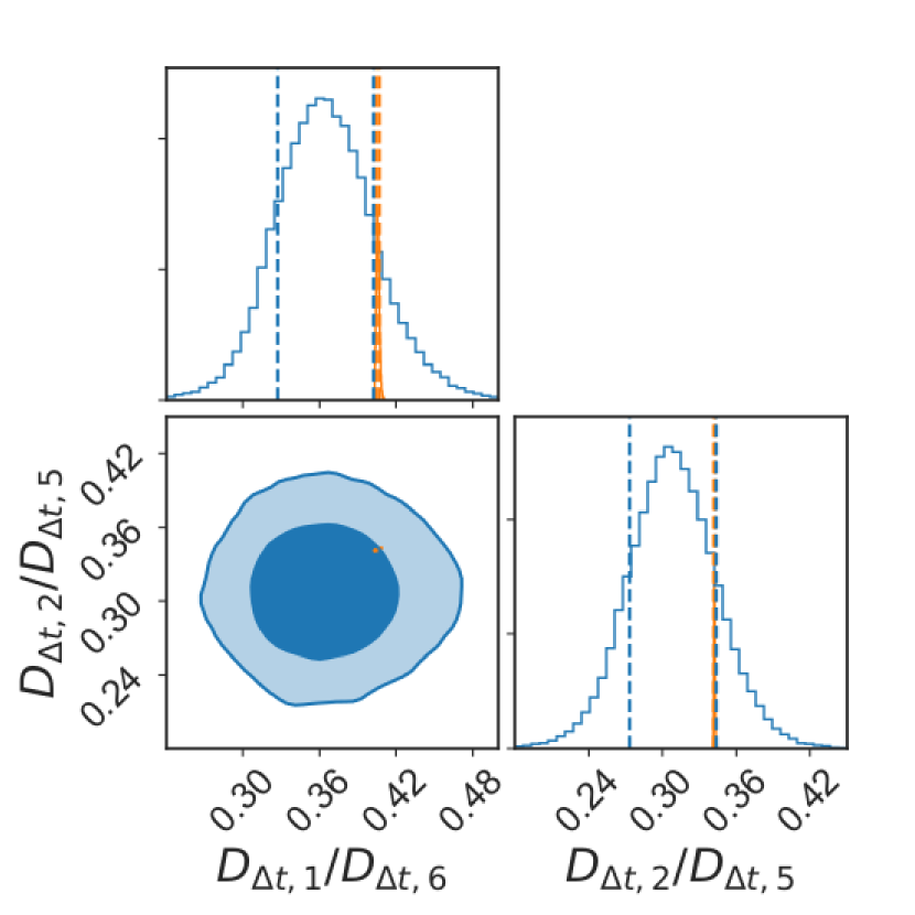
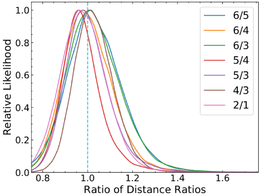
To investigate this further, in Fig. 5, we plot the measured SL 1D posteriors of every combination of the ratios of the time-delay distances of sources with lens redshifts both at or both at (left panel), or one at and one at (right panel). These 1D posterior ratios are given relative to the predictions of those same ratios from the SNe data, i.e. , so consistency gives the value of 1. This can also be viewed equivalently as , testing that SL cosmology is consistent with SNe cosmology, irrespective of .
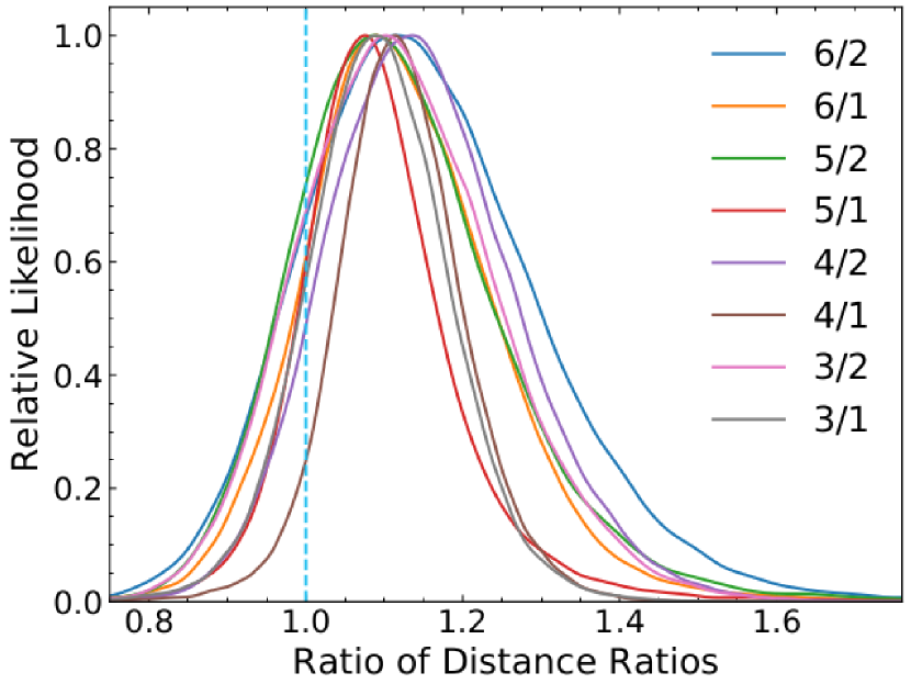
Interestingly, when both lens systems in the ratio have , or both have , then the posteriors of the 7 possible combinations all peak very close to unity, showing consistency (see left panel). However, when the lenses in the ratio lie on opposite sides of , then although the posteriors are still consistent with the value 1, the peaks tend to be higher. Any one posterior could fluctuate above the consistency value of 1, but we note that all 8 possible combinations all lie high. This is not to say that one should multiply 8 deviations (Wong et al. (2019) find this trend to be somewhat under ); we merely consider it odd enough to make it worthwhile looking for physics (remember, this is independent of the value of ) that could account for this. This is what we explore in the next section. Alternately, it could be due to some unidentified observational systematic, and one should see if this putative trend persists with new lens systems and new data.
5. A Question of Gravity
In going from the four lens systems of Birrer et al. (2019) to the seven lens systems of Wong et al. (2019) and Shajib et al. (2019) (the posterior chains for the last, DES J0408-5354, have not been publicly released yet but we include in this section their quoted value from it), the apparent trend of the time-delay distance with respect to the distance relation predicted by the supernova luminosity distance (Liao et al., 2019), or derived Hubble constant (Wong et al., 2019), as a function of time-delay distance or lens redshift has remained. In particular, see Fig. 5 of Millon et al. (2019). The statistical sample is still small, so perhaps this can be just an odd fluctuation despite the extra systems not reducing the trend.
In this section we briefly explore the conjecture that the trend is physical, and that it could be related not to the background expansion history (distances, so SN and BAO are unaffected) but rather the behavior of gravity on light deflection (lensing) evolving with redshift. This is commonly called and arises in many modified gravity theories.
The light deflection depends on the sum of the time-time and space-space metric potentials, , and is related to the density contrast by
| (7) |
Could the trend be reflecting ? Note that does not affect supernova distances, so those would reflect the actual background expansion history.
Here we simply give a rough analysis, ignoring some subtleties we mention later. The measured lensing time delays depend on
| (8) |
where is the difference in Fermat potentials. The Fermat potential difference
| (9) |
where is the angular difference between the image location and unlensed source location, and is a projected potential. The angular deflection with modified gravity light propagation becomes
| (10) |
and the projected potential is related to the convergence from mass along the line of sight by
| (11) |
Thus the gravitational effects on light propagation give
| (12) |
Since the Hubble constant estimated from a lens system comes from then for given measured lens system characteristics we have
| (13) |
That is, if is increasing with then the derived value of will increase for lower redshift lens systems.
We can assume this is the cause of the observed trend in derived from the lens systems and derive what function is needed. At high redshift we expect gravity to restore to general relativity (e.g. to preserve the successes of the cosmic microwave background and primordial nucleosynthesis) so we take values of derived at high redshift to be the true values. Figure 6 shows the values given in Millon et al. (2019), within CDM, for the seven lens systems and an illustrative power law in scale factor,
| (14) |
(Note that for many modified gravity models actually levels out to a constant de Sitter value not far into the future.)
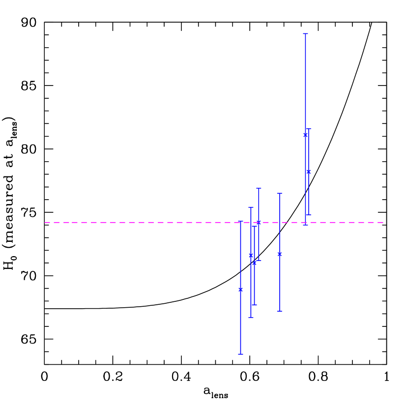
The rise in measured values comes in quite steeply with scale factor, around (or ). A change so rapid to distances themselves is quite difficult to achieve, since distances are integrals over the expansion rate (and double integrals over dark energy equation of state). And certainly no such dramatic change in seen in supernova distances. However, by changing the gravitational strength affecting light deflection, , this is less difficult. Indeed, such a rapid change has been shown to occur for some actual modified gravity theories – see for example Fig. 5 (right panel, thin curves) of Linder (2017). Note the numerical solution there shows that indeed the effect on can first become significant at low redshifts. While that particular theory (uncoupled Galileon) is ruled out, it does give a proof of principle that modified gravity can act in such a manner.
One might also speculate that the effect on light deflection could show up in weak lensing measurements. For the convergence or shear power spectrum, the relativistic Poisson equation (7) shows that and so the measured shear power will be proportional to . There is an extra element in that the growth of structure also depends on , but we focus here on . The value of the mass fluctuation amplitude , or , derived from the shear power spectrum will thus be proportional to . This was discussed in Daniel & Linder (2010) – “For higher [], lower values of will produce comparable lensing potentials. Larger [] does not cause to decrease per se, rather it brings lower values of into better agreement with the data”. Since we take to be strengthening at lower redshift for the SL case, this means that the value of or derived from low redshift surveys should be less than from high redshift surveys (or Planck CMB). This trend does seem consistent with weak lensing survey data (but again, evolution of can overturn this).
Regarding the subtleties we mentioned at the beginning of this section, note that the light deflection occurs all along the path and not just at the lens, but as with general relativistic light deflection one can treat the deflection as occurring at the lens, in a single screen approximation. Right at the lens we might expect the modified gravity to be screened, but further out from the lens the screening vanishes and the dominant part of the path integral is roughly at the lens redshift. Thus we take .
Finally, it is not clear how could help with the Cepheid measurement of higher , though the value from the tip of the red giant branch technique is more consistent. This whole section is simply speculation, but if the trend in measurements with distance persists, we might consider it a question of gravity.
6. Conclusion and Discussions
Based on the method we previously proposed, we give a cosmology model-independent determination of with the updated H0LiCOW dataset consisting of six lenses. The absolute lensing distances ( and ) are used to anchor the Pantheon SNe samples that give the shape of the distance-redshift relation through GP regression. The results are for a flat universe and for a non-flat universe. These values are consistent with the results assuming a CDM model, and have comparable uncertainties, though they have the advantage of being cosmology model independent (and include SN). With current data, measurements do not play a significant role, though they have the property of being relatable to SN independent of spatial curvature.
We perform several consistency tests of the data, and between the different probes. All show consistency, though an odd systematic trend persists in the value of the derived with lens redshift. We illustrate this trend through several methods. In particular, one could interpret it as a transition at . Irrespective of the value of , the distances from SL systems lying all below or all above are highly consistent with the SNe cosmology (this holds for all 7 such combinations of systems), but comparison of lensing systems on either side of all show an offset (admittedly individually statistically minor) from the SN cosmology – this holds, in the same direction, for all 8 such combinations of systems.
This could be a statistical fluke (though it has persisted since the first analysis with fewer systems) or some observational systematic. We speculate about one possible explanation based on physics beyond the standard model, showing how a modification in the effect of gravity on light propagation, , could account for this. Moreover, models in the literature show that the magnitude and redshift dependence of such an effect is possible, and this could also affect the perceived value of , possibly bearing on that tension as well. Given the low statistical significance with current data, we merely suggest keeping an eye on whether further, or improved, data continue to support such a physics explanation.
Fortunately time-delay strong lensing is a burgeoning field with the onset of cosmic surveys, and more well-measured and well-analyzed lenses are not far off, with imaging surveys such as DES, ZTF, LSST, and Euclid. Monitoring campaigns, adaptive optics, and spectroscopic followup (including multiobject instruments such as DESI) all play important roles as well. More lens systems at all redshifts – near , below, and well above will test whether a standard cosmology matches both strong lenses and supernovae. Continued detailed systematics studies of all distance indicators – and all light deflection probes – will be essential for confirming any result.
Acknowledgments
KL was supported by the National Natural Science Foundation of China (NSFC) No. 11973034. AS would like to acknowledge the support of the Korea Institute for Advanced Study (KIAS) grant funded by the Korea government and Kobayashi-Maskawa Institute (KMI) and Nagoya University for their hospitality in the final stages of this project. EL is supported in part by the Energetic Cosmos Laboratory and by the U.S. Department of Energy, Office of Science, Office of High Energy Physics, under Award DE-SC-0007867 and contract no. DE-AC02-05CH11231.
References
- Addison et al. (2018) Addison, G.E., Watts, D.J., Bennett, C.L., Halpern, M., Hinshaw, G., Weiland, J.L., 2018, ApJ, 853, 119 [arXiv:1707.06547]
- Aubourg et al. (2015) Aubourg, É., Bailey, S., Bautista, J. E., et al. 2015, Phys. Rev. D, 92, 123516
- Birrer et al. (2016) Birrer S., Amara A., Refregier A., 2016, JCAP, 08, 020
- Birrer et al. (2019) Birrer S., Treu T., Rusu C. E., et al., 2019, MNRAS, 484, 4726 [arXiv:1809.01274]
- Chen et al. (2019) Chen G. C.-F., Fassnacht D., Suyu S. H., et al., 2019, arXiv:1907.02533
- Collett et al. (2019) Collett T., Montanari F., Räsänen S., 2019, PhRvL, 123, 231101
- Cuceu et al. (2019) Cuceu, A., Farr, J., Lemos, P., Font-Ribera, A., 2019, arXiv:1906.11628
- Cuesta et al. (2015) Cuesta, A. J., Verde, L., Riess, A., Jimenez, R. 2015, MNRAS, 448, 3463
- Daniel & Linder (2010) Daniel, S.F., Linder, E.V., 2010, Phys. Rev. D, 82, 103523 [arXiv:1008.0397]
- Freedman et al. (2020) Freedman W. L., Madore B. F., Hoyt T., et al., 2020, arXiv:2002.01550
- Jee et al. (2015) Jee I., Komatsu E., Suyu S.-H. 2015, JCAP, 11, 033
- Jee et al. (2016) Jee I., Komatsu E., Suyu S. H., Huterer D. 2016, JCAP, 04, 031
- Jee et al. (2019) Jee I., Suyu S., Komatsu E., et al., 2019, Science, 365, 1134
- Joudaki et al. (2018) Joudaki, S., Kaplinghat, M., Keeley, R., et al. 2018, Phys. Rev. D, 97, 123501
- Kirkby & Keeley (2017) Kirkby, D., Keeley, R. 2017, 10.5281/zenodo.999564
- Koo et al. (2020) Koo, H., Shafieloo, A., Keeley, R.E., L’Huillier, B. 2020, arXiv:2001.10887
- Liao et al. (2019) Liao, K., Shafieloo, A., Keeley, R.E., Linder, E.V., 2019, ApJ, 886, L23 [arXiv:1908.04967]
- Linder (2017) Linder, E.V., 2017, Phys. Rev. D, 95, 023518 [arXiv:1607.03113]
- Macaulay et al. (2019) Macaulay, E., et al., 2019, MNRAS, 486, 2184 [arXiv:1811.02376]
- Millon et al. (2019) Millon, M., Galan, A., Courbin, F., et al., arXiv:1912.08027
- Pandey, Raveri, Jain (2019) Pandey, S., Raveri, M., Jain, B. 2019, arXiv:1912.04325
- Paraficz & Hjorth (2009) Paraficz D., Hjorth J., 2009, A&A, 507, L49
- Philcox et al. (2020) Philcox, O.H.E., Ivanov, M.M, Simonović, M., Zaldarriaga, M., 2020, arXiv:2002.04035
- Planck (2018) Planck Collaboration et al., 2018, preprint, arXiv:1807.06209
- Refsdal (1964) Refsdal S., 1964, MNRAS, 128, 307
- Riess et al. (2019) Riess A. G., Casertano S., Yuan W., Macri L. M., Scolnic D., 2019, ApJ, 876, 85
- Rusu et al. (2017) Rusu C. E., Fassnacht C. D., Sluse D., et al. 2017, MNRAS, 467, 4220
- Rusu et al. (2019) Rusu C. E., Wong K. C., Bonvin V., et al., 2019, arXiv: 1905.09338
- Scolnic et al. (2018) Scolnic D. M., et al., 2018, ApJ, 859, 101
- Shajib et al. (2019) Shajib, A.J., Birrer, S., Treu, T., et al., arXiv:1910.06306
- Suyu et al. (2010) Suyu S. H., Marshall P. J., Auger M. W., et al., 2010, ApJ, 711, 201
- Suyu et al. (2014) Suyu S. H., Treu T., Hilbert S., et al., 2014, ApJL, 788, L35
- Suyu et al. (2017) Suyu S. H., Bonvin V., Courbin F., et al., 2017, MNRAS, 468, 2590
- Taubenberger et al. (2019) Taubenberger S., Suyu S. H., Komatsu E., et al., 2019, arXiv:1905.12496
- Treu (2010) Treu T. 2010, Annu. Rev. Astron. Astrophys., 48, 87
- Treu & Marshall (2016) Treu T., Marshall P. J., 2016, Astron. Astrophys. Rev., 24, 11
- Weinberg (1972) Weinberg, S. 1972, Gravitation and Cosmology: Principles and Applications of the General Theory of Relativity
- Wong et al. (2019) Wong K. C., Suyu S. H., Chen G. C.-F., et al., 2019, arXiv:1907.04869
- Wong et al. (2017) Wong K. C., Suyu S. H., Auger M. W., et al., 2017, MNRAS, 465, 4895