Deterministic Approximation for Submodular Maximization over a Matroid in Nearly Linear Time
We study the problem of maximizing a non-monotone, non-negative submodular function subject to a matroid constraint. The prior best-known deterministic approximation ratio for this problem is under time complexity. We show that this deterministic ratio can be improved to under time complexity, and then present a more practical algorithm dubbed TwinGreedyFast which achieves deterministic ratio in nearly-linear running time of . Our approach is based on a novel algorithmic framework of simultaneously constructing two candidate solution sets through greedy search, which enables us to get improved performance bounds by fully exploiting the properties of independence systems. As a byproduct of this framework, we also show that TwinGreedyFast achieves deterministic ratio under a -set system constraint with the same time complexity. To showcase the practicality of our approach, we empirically evaluated the performance of TwinGreedyFast on two network applications, and observed that it outperforms the state-of-the-art deterministic and randomized algorithms with efficient implementations for our problem.
1 Introduction
Submodular function maximization has aroused great interests from both academic and industrial societies due to its wide applications such as crowdsourcing [47], information gathering [35], sensor placement [33], influence maximization [37, 48] and exemplar-based clustering [30]. Due to the large volume of data and heterogeneous application scenarios in practice, there is a growing demand for designing accurate and efficient submodular maximization algorithms subject to various constraints.
Matroid is an important structure in combinatorial optimization that abstracts and generalizes the notion of linear independence in vector spaces [8]. The problem of submodular maximization subject to a matroid constraint (SMM) has attracted considerable attention since the 1970s. When the considered submodular function is monotone, the classical work of Fisher et al. [27] presents a deterministic approximation ratio of , which keeps as the best deterministic ratio during decades until Buchbinder et al. [14] improve this ratio to very recently.
When the submodular function is non-monotone, the best-known deterministic ratio for the SMM problem is , proposed by Lee et al. [38], but with a high time complexity of . Recently, there appear studies aiming at designing more efficient and practical algorithms for this problem. In this line of studies, the elegant work of Mirzasoleiman et al. [44] and Feldman et al. [25] proposes the best deterministic ratio of and the fastest implementation with an expected ratio of , and their algorithms can also handle more general constraints such as a -set system constraint. For clarity, we list the performance bounds of these work in Table 1. However, it is still unclear whether the deterministic ratio for a single matroid constraint can be further improved, or whether there exist faster algorithms achieving the same deterministic ratio.
In this paper, we propose an approximation algorithm TwinGreedy (Alg. 1) with a deterministic ratio and running time for maximizing a non-monotone, non-negative submodular function subject to a matroid constraint, thus improving the best-known deterministic ratio of Lee et al. [38]. Furthermore, we show that the solution framework of TwinGreedy can be implemented in a more efficient way, and present a new algorithm dubbed TwinGreedyFast with deterministic ratio and nearly-linear running time. To the best of our knowledge, TwinGreedyFast is the fastest algorithm achieving the deterministic ratio for our problem in the literature. As a byproduct, we also show that TwinGreedyFast can be used to address a more general -set system constraint and achieves a approximation ratio with the same time complexity.
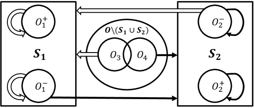
It is noted that most of the current deterministic algorithms for non-monontone submodular maximization (e.g., [44, 25, 45]) leverage the “repeated greedy-search” framework proposed by Gupta et al. [31], where two or more candidate solution sets are constructed successively and then an unconstrained submodular maximization (USM) algorithm (e.g., [12]) is called to find a good solution among the candidate sets and their subsets. Our approach is based on a novel “simultaneous greedy-search” framework different from theirs, where two disjoint candidate solution sets and are built simultaneously with only single-pass greedy searching, without calling a USM algorithm. We call these two solution sets and as “twin sets” because they “grow up” simultaneously. Thanks to this framework, we are able to bound the “utility loss” caused by greedy searching using and themselves, through a careful classification of the elements in an optimal solution and mapping them to the elements in . Furthermore, by incorporating a thresholding method inspired by Badanidiyuru and Vondrák [2] into our framework, the TwinGreedyFast algorithm achieves nearly-linear time complexity by only accepting elements whose marginal gains are no smaller than given thresholds.
We evaluate the performance of TwinGreedyFast on two applications: social network monitoring and multi-product viral marketing. The experimental results show that TwinGreedyFast runs more than an order of magnitude faster than the state-of-the-art efficient algorithms for our problem, and also achieves better solution quality than the currently fastest randomized algorithms in the literature.
| Algorithms | Ratio | Time Complexity | Type |
| Lee et al. [38] | Deterministic | ||
| Mirzasoleiman et al. [44] | Deterministic | ||
| Feldman et al. [25] | Randomized | ||
| Buchbinder and Feldman [10] | Randomized | ||
| TwinGreedy (Alg. 1) | Deterministic | ||
| TwinGreedyFast (Alg. 2) | Deterministic |
1.1 Related Work
When the considered submodular function is monotone, Calinescu et al. [15] propose an optimal expected ratio for the problem of submodular maximization subject to a matroid constraint (SMM). The SMM problem seems to be harder when is non-monotone, and the current best-known expected ratio is 0.385 [10], got after a series of studies [50, 29, 24, 38]. However, all these approaches are based on tools with high time complexity such as multilinear extension.
There also exist efficient deterministic algorithms for the SMM problem: Gupta et al. [31] are the first to apply the “repeated greedy search” framework described in last section and achieve ratio, which is improved to by Mirzasoleiman et al. [44] and Feldman et al. [25]; under a more general -set system constraint, Mirzasoleiman et al. [44] achieve deterministic ratio and Feldman et al. [25] achieve deterministic ratio (assuming that they use the USM algorithm with deterministic ratio in [9]); some studies also propose streaming algorithms under various constraints [45, 32].
As regards the efficient randomized algorithms for the SMM problem, the SampleGreedy algorithm in [25] achieves expected ratio with running time; the algorithms in [11] also achieve a expected ratio with slightly worse time complexity of and a expected ratio under cubic time complexity of 111Although the randomized 0.283-approximation algorithm in [11] has a better approximation ratio than TwinGreedy, its time complexity is larger than that of TwinGreedy by at least an additive factor of , which can be large as can be in the order of .; Chekuri and Quanrud [16] provide a expected ratio under adaptive rounds; and Feldman et al. [26] propose a expected ratio under the steaming setting. It is also noted that Buchbinder et al. [14] provide a de-randomized version of the algorithm in [11] for monotone submodular maximization, which has time complexity of . However, it remains an open problem to find the approximation ratio of this de-randomized algorithm for the SMM problem with a non-monotone objective function.
A lot of elegant studies provide efficient submodular optimization algorithms for monotone submodular functions or for a cardinality constraint [2, 13, 4, 43, 5, 36, 23, 22]. However, these studies have not addressed the problem of non-monotone submodular maximization subject to a general matroid (or -set system) constraint, and our main techniques are essentially different from theirs.
2 Preliminaries
Given a ground set with , a function is submodular if for all , . The function is called non-negative if for all , and is called non-monotone if . For brevity, we use to denote for any , and write as for any . We call as the “marginal gain” of with respect to .
An independence system consists of a finite ground set and a family of independent sets satisfying: (1) ; (2) If , then (called hereditary property). An independence system is called a matroid if it satisfies: for any and , there exists such that (called exchange property).
Given an independence system and any , is called a base of if: (1) ; (2) . The independence system is called a -set system if for every and any two basis of , we have (). It is known that -set system is a generalization of several structures on independence systems including matroid, -matchoid and -extendible system, and an inclusion hierarchy of these structures can be found in [32].
In this paper, we consider a non-monotone, non-negative submodular function . Given and a matroid , our optimization problem is . In the end of Section 4, we will also consider a more general case where is a -set system.
We introduce some frequently used properties of submodular functions. For any and any , we have ; this property can be derived by the definition of submodular functions. For any and a partition of , we have
| (1) |
For convenience, we use to denote for any positive integer , and use to denote the rank of , i.e., , and denote an optimal solution to our problem by .
3 The TwinGreedy Algorithm
In this section, we consider a matroid constraint and introduce the TwinGreedy algorithm (Alg. 1) that achieves approximation ratio. The TwinGreedy algorithm maintains two solution sets and that are initialized to empty sets. At each iteration, it considers all the candidate elements in that can be added into or without violating the feasibility of . If there exists such an element, then it greedily selects where such that adding into can bring the maximal marginal gain without violating the feasibility of . TwinGreedy terminates when no more elements can be added into or with a positive marginal gain while still keeping the feasibility of . Then it returns the one between and with the larger objective function value.
Although the TwinGreedy algorithm is simple, its performance analysis is highly non-trivial. Roughly speaking, as TwinGreedy adopts a greedy strategy to select elements, we try to find some “competitive relationships” between the elements in and those in , such that the total marginal gains of the elements in with respect to and can be upper-bounded by and ’s own objective function values. However, this is non-trivial due to the correlation between the elements in and . To overcome this hurdle, we first classify the elements in , as shown in Definition 1:
Definition 1
Consider the two solution sets and when TwinGreedy returns. We can write as where , such that is added into by the algorithm before for any . With this ordered list, given any , we define
| (2) |
That is, denotes the set of elements in () that are added by the TwinGreedy algorithm before adding . Furthermore, we define
We also define the marginal gain of any as , where if and otherwise ().
Intuitively, each element can also be added into without violating the feasibility of when is added into , while the elements in do not have this nice property. The sets and can be understood similarly. With the above classification of the elements in , we further consider two groups of elements: and . By leveraging the properties of independence systems, we can map the first group to and the second group to , as shown by Lemma 1 (the proof can be found in the supplementary file). Intuitively, Lemma 1 holds due to the exchange property of matroids.
Lemma 1
There exists an injective function such that:
-
1.
For any , we have .
-
2.
For each , we have .
Similarly, there exists an injective function such that for each and for each .
The first property shown in Lemma 1 implies that, at the moment that is added into , can also be added into without violating the feasibility of (for any ). This makes it possible to compare the marginal gain of with respect to with that of . The construction of is also based on this intuition. With the two injections and , we can bound the marginal gains of to with respect to and , as shown by the Lemma 2. Lemma 2 can be proved by using Definition 1, Lemma 1 and the submodularity of .
Lemma 2
The proof of Lemma 2 is deferred to the supplementary file. In the next section, we will provide a proof sketch for a similar lemma (i.e., Lemma 3), which can also be used to understand Lemma 2. Now we can prove the performance bounds of TwinGreedy:
Theorem 1
When is a matroid, the algorithm returns a solution with approximation ratio, under time complexity of .
Proof: If or , then we get an optimal solution, which is shown in the supplementary file. So we assume and . Let and . By Eqn. (1), we get
| (6) | |||
| (7) |
Using Lemma 2, we can get
| (8) |
where the second inequality is due to that and are both injective functions shown in Lemma 1, and that for every according to Line 1 of TwinGreedy. Besides, according to the definition of , we must have for each , because otherwise should be added into as . Similarly, we get for each . Therefore, we have
| (9) |
4 The TwinGreedyFast Algorithm
As the TwinGreedy algorithm still has quadratic running time, we present a more efficient algorithm TwinGreedyFast (Alg. 2). As that in TwinGreedy, the TwinGreedyFast algorithm also maintains two solution sets and , but it uses a threshold to control the quality of elements added into or . More specifically, given a threshold , TwinGreedyFast checks every unselected element in an arbitrarily order. Then it chooses such that adding into does not violate the feasibility of while is maximized. If the marginal gain is no less than , then is added into , otherwise the algorithm simply neglects . The algorithm repeats the above process starting from and decreases by a factor at each iteration until is sufficiently small, then it returns the one between and with the larger objective value.
The performance analysis of TwinGreedyFast is similar to that of TwinGreedy. Let us consider the two solution sets and when TwinGreedyFast returns. We can define , , , , , , and in exact same way as Definition 1, and Lemma 1 still holds as the construction of and only depends on the insertion order of the elements in , which is fixed when TwinGreedyFast returns. We also try to bound the marginal gains of - with respect to and in a way similar to Lemma 2. However, due to the thresholds introduced in TwinGreedyFast, these bounds are slightly different from those in Lemma 2, as shown in Lemma 3:
Lemma 3
The TwinGreedyFast algorithm satisfies:
| (12) | |||||
| (13) | |||||
| (14) |
where and are the two functions defined in Lemma 1.
Proof: (sketch) At the moment that any is added into , it can also be added into due to Definition 1. Therefore, we must have according to the greedy selection rule of TwinGreedyFast. Using submodularity, we get the first inequality in the lemma:
For any , consider the moment that TwinGreedyFast adds into . According to Lemma 1, we have . This implies that has not been added into yet, because otherwise we have and hence according to the hereditary property of independence systems, which contradicts . As such, we must have and where is the threshold used by TwinGreedyFast when adding , because otherwise should have been added before in an earlier stage of the algorithm with a larger threshold. Combining these results gives us
The other inequalities in the lemma can be proved similarly.
With Lemma 3, we can use similar reasoning as that in Theorem 1 to prove the performance bounds of TwinGreedyFast, as shown in Theorem 2. The full proofs of Lemma 3 and Theorem 2 can be found in the supplementary file.
Theorem 2
When is a matroid, the algorithm returns a solution with approximation ratio, under time complexity of .
Extensions:
The TwinGreedyFast algorithm can also be directly used to address the problem of non-monotone submodular maximization subject to a -set system constraint (by simply inputting a -set system into TwinGreedyFast). It achieves a deterministic ratio under time complexity in such a case, which improves upon both the ratio and time complexity of the results in [44, 31]. We note that the prior best known result for this problem is a -approximation under time complexity proposed in [25]. Compared to this best known result, TwinGreedyFast achieves much smaller time complexity, and also has a better approximation ratio when . The proof for this performance ratio of TwinGreedyFast (shown in the supplementary file) is almost the same as those for Theorems 1-2, as we only need to relax Lemma 1 to allow that the preimage by or of any element in contains at most elements.
5 Performance Evaluation
In this section, we evaluate the performance of TwinGreedyFast under two social network applications, using both synthetic and real networks. We implement the following algorithms for comparison:
-
1.
SampleGreedy: This algorithm is proposed in [25] which has expected ratio and running time. To the best of our knowledge, it is currently the fastest randomized algorithm for non-monotone submodular maximization over a matroid.
-
2.
Fantom: Excluding the ratio proposed in [38], the Fantom algorithm from [44] has the best deterministic ratio for our problem. As it needs to call an unconstrained submodular maximization (USM) algorithm, we use the USM algorithm proposed in [12] with deterministic ratio and linear running time. As such, Fantom achieves deterministic ratio in the experiments.222We have also tested Fantom using the randomized USM algorithm in [12] with expected ratio. The experimental results are almost identical, although Fantom has a larger ratio (in expectation) in such a case.
-
3.
ResidualRandomGreedy: This algorithm is from [11] which has expected ratio and running time. We denote it as “RRG” for brevity.
-
4.
TwinGreedyFast: We implement our Algorithm 2 by setting . As such, it achieves 0.15 deterministic approximation ratio in the experiments.
5.1 Applications
Given a social network where is the set of nodes and is the set of edges, we consider the following two applications in our experiments. Both applications are instances of non-monotone submodular maximization subject to a matroid constraint, which is proved in the supplementary file.
-
1.
Social Network Monitoring: This application is similar to those applications considered in [40] and [36]. Suppose that each edge is associated with a weight denoting the maximum amount of content that can be propagated through . Moreover, is partitioned into disjoint subsets according to the users’ properties such as ages and political leanings. We need to select a set of users to monitor the network, such that the total amount of monitored content is maximized. Due to the considerations on diversity or fairness, we also require , where is a predefined constant.
-
2.
Multi-Product Viral Marketing: This application is a variation of the one considered in [18]. Suppose that a company with a budget needs to select a set of at most seed nodes to promote products. Each node can be selected as a seed for at most one product and also has a cost for serving as a seed. The goal is to maximize the revenue (with budget-saving considerations): , where is the set of seed nodes selected for product , and is a monotone and submodular influence spread function as that proposed in [34]. We also assume that is large enough to keep the revenue non-negative, and assume that selecting no seed nodes would cause zero revenue.
5.2 Experimental Results
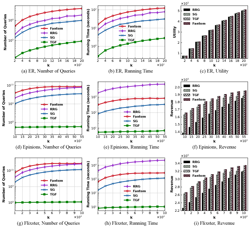
The experimental results are shown in Fig. 2. In overview, TwinGreedyFast runs more than an order of magnitude faster than the other three algorithms; Fantom has the best performance on utility; the performance of TwinGreedyFast on utility is close to that of Fantom.
5.2.1 Social Network Monitoring
We generate an Erdős–Rényi (ER) random graph with 3000 nodes and set the edge probability to . The weight for each is generated uniformly at random from and all nodes are randomly assigned to five groups. In the supplementary file, we also generate Barabási–Albert (BA) graphs for comparison, and the results are qualitatively similar. It can be seen from Fig. 2(a) that Fantom incurs the largest number of queries to objective function, as it leverages repeated greedy searching processes to find a solution with good quality. SampleGreedy runs faster than RRG, which coincides with their time complexity mentioned in Section 1.1. TwinGreedyFast significantly outperforms Fantom, RRG and SampleGreedy by more than an order of magnitude in Fig. 2(a) and Fig. 2(b), as it achieves nearly linear time complexity. Moreover, it can be seen from Figs. 2(a)-(b) that TwinGreedyFast maintains its advantage on efficiency no matter the metric is wall-clock running time or number of queries. Finally, Fig. 2(c) shows that all the implemented algorithms achieve approximately the same utility on the ER random graph.
5.2.2 Multi-Product Viral Marketing
We use two real social networks Flixster and Epinions. Flixster is from [6] with 137925 nodes and 2538746 edges, and Epinions is from the SNAP dataset collection [39] with 75879 nodes and 508837 edges. We consider three products and follow the Independent Cascade (IC) model [34] to set the influence spread function for each product . Note that the IC model requires an activation probability associated with each edge . This probability is available in the Flixster dataset (learned from real users’ action logs), and we follow Chen et al. [17] to set for the Epinions dataset, where is the set of in-neighbors of . As evaluating under the IC model is NP-hard, we follow the approach in [7] to generate a set of one million random Reverse-Reachable Sets (RR-sets) such that can be approximately evaluated using these RR-sets. The cost of each node is generated uniformly at random from , and we set to keep the function value non-negative. More implementation details can be found in the supplementary file.
We plot the experimental results on viral marketing in Fig. 2(d)-Fig. 2(i). The results are qualitatively similar to those in Fig. 2(a)-Fig. 2(c), which show that TwinGreedyFast is still significantly faster than the other algorithms. Fantom achieves the largest utility again, while TwinGreedyFast performs closely to Fantom and outperforms the other two randomized algorithms on utility.
6 Conclusion and Discussion
We have proposed the first deterministic algorithm to achieve an approximation ratio of for maximizing a non-monotone, non-negative submodular function subject to a matroid constraint, and our algorithm can also be accelerated to achieve nearly-linear running time. In contrast to the existing algorithms adopting the “repeated greedy-search” framework proposed by [31], our algorithms are designed based on a novel “simultaneous greedy-search” framework, where two candidate solutions are constructed simultaneously, and a pair of an element and a candidate solution is greedily selected at each step to maximize the marginal gain. Moreover, our algoirthms can also be directly used to handle a more general -set system constraint or monotone submodular functions, while still achieving nice performance bounds. For example, by similar reasoning with that in Sections 3-4, it can be seen that our algorithms can achieve ratio for monotone under a -set system constraint, which is almost best possible [2]. We have evaluated the performance of our algorithms in two concrete applications for social network monitoring and multi-product viral marketing, and the extensive experimental results demonstrate that our algorithms runs in orders of magnitude faster than the state-of-the-art algorithms, while achieving approximately the same utility.
Acknowledgements
This work was supported by the National Key RD Program of China under Grant No. 2018AAA0101204, the National Natural Science Foundation of China (NSFC) under Grant No. 61772491 and Grant No. U1709217, Anhui Initiative in Quantum Information Technologies under Grant No. AHY150300, and the Fundamental Research Funds for the Central Universities.
Broader Impact
Submodular optimization is an important research topic in data mining, machine learning and optimization theory, as it has numerous applications such as crowdsourcing [47], viral marketing [34], feature selection [28], network monitoring [40], document summarization [41, 20], online advertising [49], crowd teaching [46] and blogosphere mining [21]. Matroid is a fundamental structure in combinatorics that captures the essence of a notion of "independence" that generalizes linear independence in vector spaces. The matroid structure has been pervasively found in various areas such as geometry, network theory, coding theory and graph theory [8]. The study on submodular maximization subject to matroid constraints dates back to the 1970s (e.g., [27]), and it is still a hot research topic today [44, 25, 45, 5, 16, 3]. A lot of practical problems can be cast as the problem of submodular maximziation over a matroid constraint (or more general -set system constraints), such as diversity maximization [1], video summarization [52], clustering [42], multi-robot allocation [51] and planning sensor networks [19]. Therefore, our study has addressed a general and fundamental theoretical problem with many potential applications.
Due to the massive datasets used everywhere nowadays, it is very important that submodular optimization algorithms should achieve accuracy and efficiency simultaneously. Recently, there emerge great interests on designing more practical and efficient algorithms for submodular optimization (e.g., [2, 13, 4, 43, 36, 23, 11]), and our work advances the state of the art in this area by proposing a new efficient algorithm with improved performance bounds. Moreover, our algorithms are based on a novel “simultaneous greedy-search” framework, which is different from the classical “repeated greedy-search” and “local search” frameworks adopted by the state-of-the-art algorithms (e.g., [31, 38, 25, 44]). We believe that our “simultaneous greedy-search” framework has the potential to be extended to address other problems on submodular maximization with more complex constraints, which is the topic of our ongoing research.
References
- Abbassi et al. [2013] Z. Abbassi, V. S. Mirrokni, and M. Thakur. Diversity maximization under matroid constraints. In KDD, pages 32–40, 2013.
- Badanidiyuru and Vondrák [2014] A. Badanidiyuru and J. Vondrák. Fast algorithms for maximizing submodular functions. In SODA, pages 1497–1514, 2014.
- Balcan and Harvey [2018] M.-F. Balcan and N. J. Harvey. Submodular functions: Learnability, structure, and optimization. SIAM Journal on Computing, 47(3):703–754, 2018.
- Balkanski et al. [2018] E. Balkanski, A. Breuer, and Y. Singer. Non-monotone submodular maximization in exponentially fewer iterations. In NIPS, pages 2353–2364, 2018.
- Balkanski et al. [2019] E. Balkanski, A. Rubinstein, and Y. Singer. An optimal approximation for submodular maximization under a matroid constraint in the adaptive complexity model. In STOC, pages 66–77, 2019.
- Barbieri et al. [2012] N. Barbieri, F. Bonchi, and G. Manco. Topic-aware social influence propagation models. In ICDM, pages 81–90, 2012.
- Borgs et al. [2014] C. Borgs, M. Brautbar, J. Chayes, and B. Lucier. Maximizing social influence in nearly optimal time. In SODA, pages 946–957, 2014.
- Bryant and Perfect [1980] V. Bryant and H. Perfect. Independence Theory in Combinatorics: An Introductory Account with Applications to Graphs and Transversals. Springer, 1980.
- Buchbinder and Feldman [2018] N. Buchbinder and M. Feldman. Deterministic algorithms for submodular maximization problems. ACM Transactions on Algorithms, 14(3):1–20, 2018.
- Buchbinder and Feldman [2019] N. Buchbinder and M. Feldman. Constrained submodular maximization via a nonsymmetric technique. Mathematics of Operations Research, 44(3):988–1005, 2019.
- Buchbinder et al. [2014] N. Buchbinder, M. Feldman, J. Naor, and R. Schwartz. Submodular maximization with cardinality constraints. In SODA, pages 1433–1452, 2014.
- Buchbinder et al. [2015] N. Buchbinder, M. Feldman, J. Seffi, and R. Schwartz. A tight linear time (1/2)-approximation for unconstrained submodular maximization. SIAM Journal on Computing, 44(5):1384–1402, 2015.
- Buchbinder et al. [2017] N. Buchbinder, M. Feldman, and R. Schwartz. Comparing apples and oranges: Query trade-off in submodular maximization. Mathematics of Operations Research, 42(2):308–329, 2017.
- Buchbinder et al. [2019] N. Buchbinder, M. Feldman, and M. Garg. Deterministic (+ )-approximation for submodular maximization over a matroid. In SODA, pages 241–254, 2019.
- Calinescu et al. [2011] G. Calinescu, C. Chekuri, M. Pal, and J. Vondrák. Maximizing a monotone submodular function subject to a matroid constraint. SIAM Journal on Computing, 40(6):1740–1766, 2011.
- Chekuri and Quanrud [2019] C. Chekuri and K. Quanrud. Parallelizing greedy for submodular set function maximization in matroids and beyond. In STOC, pages 78–89, 2019.
- Chen et al. [2009] W. Chen, Y. Wang, and S. Yang. Efficient influence maximization in social networks. In KDD, pages 199–208, 2009.
- Chen et al. [2020] W. Chen, W. Zhang, and H. Zhao. Gradient method for continuous influence maximization with budget-saving considerations. In AAAI, 2020.
- Corah and Michael [2018] M. Corah and N. Michael. Distributed submodular maximization on partition matroids for planning on large sensor networks. In CDC, pages 6792–6799, 2018.
- El-Arini and Guestrin [2011] K. El-Arini and C. Guestrin. Beyond keyword search: Discovering relevant scientific literature. In KDD, pages 439–447, 2011.
- El-Arini et al. [2009] K. El-Arini, G. Veda, D. Shahaf, and C. Guestrin. Turning down the noise in the blogosphere. In KDD, pages 289–298, 2009.
- Ene and Nguyen [2019] A. Ene and H. L. Nguyen. Towards nearly-linear time algorithms for submodular maximization with a matroid constraint. In ICALP, page 54:1–54:14, 2019.
- Fahrbach et al. [2019] M. Fahrbach, V. Mirrokni, and M. Zadimoghaddam. Non-monotone submodular maximization with nearly optimal adaptivity and query complexity. In ICML, pages 1833–1842, 2019.
- Feldman et al. [2011] M. Feldman, J. Naor, and R. Schwartz. A unified continuous greedy algorithm for submodular maximization. In FOCS, pages 570–579, 2011.
- Feldman et al. [2017] M. Feldman, C. Harshaw, and A. Karbasi. Greed is good: Near-optimal submodular maximization via greedy optimization. In COLT, pages 758–784, 2017.
- Feldman et al. [2018] M. Feldman, A. Karbasi, and E. Kazemi. Do less, get more: Streaming submodular maximization with subsampling. In NIPS, pages 732–742, 2018.
- Fisher et al. [1978] M. Fisher, G. Nemhauser, and L. Wolsey. An analysis of approximations for maximizing submodular set functions—ii. Mathematical Programming Study, 8:73–87, 1978.
- Fujii and Sakaue [2019] K. Fujii and S. Sakaue. Beyond adaptive submodularity: Approximation guarantees of greedy policy with adaptive submodularity ratio. In ICML, pages 2042–2051, 2019.
- Gharan and Vondrák [2011] S. O. Gharan and J. Vondrák. Submodular maximization by simulated annealing. In SODA, pages 1098–1116, 2011.
- Gomes and Krause [2010] R. Gomes and A. Krause. Budgeted nonparametric learning from data streams. In ICML, page 391–398, 2010.
- Gupta et al. [2010] A. Gupta, A. Roth, G. Schoenebeck, and K. Talwar. Constrained non-monotone submodular maximization: Offline and secretary algorithms. In WINE, pages 246–257, 2010.
- Haba et al. [2020] R. Haba, E. Kazemi, M. Feldman, and A. Karbasi. Streaming submodular maximization under a -set system constraint. In ICML, (arXiv:2002.03352), 2020.
- Iyer and Bilmes [2013] R. K. Iyer and J. A. Bilmes. Submodular optimization with submodular cover and submodular knapsack constraints. In NIPS, pages 2436–2444, 2013.
- Kempe et al. [2003] D. Kempe, J. Kleinberg, and É. Tardos. Maximizing the spread of influence through a social network. In KDD, pages 137–146, 2003.
- Krause and Guestrin [2011] A. Krause and C. Guestrin. Submodularity and its applications in optimized information gathering. ACM Transactions on Intelligent Systems and Technology, 2(4):1–20, 2011.
- Kuhnle [2019] A. Kuhnle. Interlaced greedy algorithm for maximization of submodular functions in nearly linear time. In NIPS, pages 2371–2381, 2019.
- Kuhnle et al. [2018] A. Kuhnle, J. D. Smith, V. Crawford, and M. Thai. Fast maximization of non-submodular, monotonic functions on the integer lattice. In ICML, pages 2786–2795, 2018.
- Lee et al. [2010] J. Lee, V. S. Mirrokni, V. Nagarajan, and M. Sviridenko. Maximizing nonmonotone submodular functions under matroid or knapsack constraints. SIAM Journal on Discrete Mathematics, 23(4):2053–2078, 2010.
- Leskovec and Krevl [2014] J. Leskovec and A. Krevl. Snap datasets: Stanford large network dataset collection. URL: http://snap.stanford.edu/, 2014.
- Leskovec et al. [2007] J. Leskovec, A. Krause, C. Guestrin, C. Faloutsos, J. VanBriesen, and N. Glance. Cost-effective outbreak detection in networks. In KDD, pages 420–429, 2007.
- Lin and Bilmes [2011] H. Lin and J. Bilmes. A class of submodular functions for document summarization. In ACL/HLT, pages 510–520, 2011.
- Liu et al. [2014] M.-Y. Liu, O. Tuzel, S. Ramalingam, and R. Chellappa. Entropy-rate clustering: Cluster analysis via maximizing a submodular function subject to a matroid constraint. IEEE Transactions on Pattern Analysis and Machine Intelligence, 36(1):99–112, 2014.
- Mirzasoleiman et al. [2015] B. Mirzasoleiman, A. Badanidiyuru, A. Karbasi, J. Vondrák, and A. Krause. Lazier than lazy greedy. In AAAI, pages 1812–1818, 2015.
- Mirzasoleiman et al. [2016] B. Mirzasoleiman, A. Badanidiyuru, and A. Karbasi. Fast constrained submodular maximization: Personalized data summarization. In ICML, pages 1358–1367, 2016.
- Mirzasoleiman et al. [2018] B. Mirzasoleiman, S. Jegelka, and A. Krause. Streaming non-monotone submodular maximization: Personalized video summarization on the fly. In AAAI, pages 1379–1386, 2018.
- Singla et al. [2014] A. Singla, I. Bogunovic, G. Bartok, A. Karbasi, and A. Krause. Near-optimally teaching the crowd to classify. In ICML, pages 154–162, 2014.
- Singla et al. [2016] A. Singla, S. Tschiatschek, and A. Krause. Noisy submodular maximization via adaptive sampling with applications to crowdsourced image collection summarization. In AAAI, page 2037–2041, 2016.
- Soma and Yoshida [2017] T. Soma and Y. Yoshida. Non-monotone dr-submodular function maximization. In AAAI, pages 898–904, 2017.
- Soma and Yoshida [2018] T. Soma and Y. Yoshida. Maximizing monotone submodular functions over the integer lattice. Mathematical Programming, 172(1-2):539–563, 2018.
- Vondrák [2013] J. Vondrák. Symmetry and approximability of submodular maximization problems. SIAM Journal on Computing, 42(1):265–304, 2013.
- Williams et al. [2017] R. K. Williams, A. Gasparri, and G. Ulivi. Decentralized matroid optimization for topology constraints in multi-robot allocation problems. In ICRA, pages 293–300, 2017.
- Xu et al. [2015] J. Xu, L. Mukherjee, Y. Li, J. Warner, J. M. Rehg, and V. Singh. Gaze-enabled egocentric video summarization via constrained submodular maximization. In CVPR, pages 2235–2244, 2015.
Appendix A: Missing Proofs
A.1 Proof of Lemma 1
Proof: We only prove the existence of , as the existence of can be proved in the same way. Suppose that the elements in are (listed according to the order that they are added into ). We use an argument inspired by [15] to construct . Let . We execute the following iterations from to . At the beginning of the -th iteration, we compute a set . If (so ), then we set and . If and , then we pick an arbitrary and set ; . If , then we simply set . After that, we set and enter the -th iteration.
From the above process, it can be easily seen that has the properties required by the lemma as long as it is a valid function. So we only need to prove that each is mapped to an element in , which is equivalent to prove as each is mapped to an element in according to the above process. In the following, we prove by induction, i.e., proving for all .
We first prove . By way of contradiction, let us assume . Then, there must exist some satisfying according to the exchange property of matroids. Moreover, according to the definition of , we also have , which implies . So we can get due to , and the hereditary property of independence systems, but this contradicts the definition of . Therefore, holds when .
Now suppose for certain . If , then we have and hence . If , then we know that there does not exist such that . This implies due to the exchange property of matroids. So we also have , which completes the proof.
A.2 Proof of Lemma 2
Lemma 4
The TwinGreedy algorithm satisfies
| (15) |
Proof of Lemma 4: We only prove the first inequality, as the second one can be proved in the same way. For any , consider the moment that TwinGreedy inserts into . At that moment, adding into also does not violate the feasibility of according to the definition of . Therefore, we must have , because otherwise would not be inserted into according to the greedy rule of TwinGreedy. Using submodularity and the fact that , we get
| (16) |
and hence
| (17) |
which completes the proof.
Lemma 5
The TwinGreedy algorithm satisfies
| (18) |
Proof of Lemma 5: We only prove the first inequality, as the second one can be proved in the same way. For any , consider the moment that TwinGreedy inserts into . At that moment, adding into also does not violate the feasibility of as according to Lemma 1. This implies that has not been inserted into yet. To see this, let us assume (by way of contradiction) that has already been added into when TwinGreedy inserts into . So we have . As , we must have due to the hereditary property of independence systems. However, this contradicts as .
As has not been inserted into yet at the moment that is inserted into , and , we know that must be a contender to when TwinGreedy inserts into . Due to the greedy selection rule of the algorithm, this means . As , we also have . Putting these together, we have
| (19) |
which completes the proof.
Lemma 6
The TwinGreedy algorithm satisfies
| (20) |
Proof of Lemma 6: We only prove the first inequality, as the second one can be proved in the same way. Consider any . According to Lemma 1, we have , which means that can be added into without violating the feasibility of when is added into . According to the greedy rule of TwinGreedy and submodularity, we must have , because otherwise should be added into , which contradicts . Therefore, we get
| (21) |
which completes the proof.
A.3 Proof of Theorem 1
Proof: We only consider the special case that or is empty, as the main proof of the theorem has been presented in the paper. Without loss of generality, we assume that is empty. According to the greedy rule of the algorithm, we have
| (22) |
and . Combining these with
| (23) |
we get , which proves that is an optimal solution when is empty.
A.4 Proof of Lemma 3
Lemma 7
For the TwinGreedyFast algorithm, we have
| (24) |
Proof of Lemma 7: The proof is similar to that of Lemma 4, and we present the full proof for completeness. We will only prove the first inequality, as the second one can be proved in the same way. For any , consider the moment that TwinGreedy inserts into and suppose that the current threshold is . Therefore, we must have . At that moment, adding into also does not violate the feasibility of according to the definition of . So we must have , because otherwise we have , and hence would be inserted into according to the greedy rule of TwinGreedyFast. Using submodularity and the fact that , we get
| (25) |
and hence
| (26) |
which completes the proof.
Lemma 8
For the TwinGreedyFast Algorithm, we have
| (27) |
Proof of Lemma 8: We only prove the first inequality, as the second one can be proved in the same way. For any , consider the moment that TwinGreedyFast adds into . Using the same reasoning with that in Lemma 5, we can prove: (1) has not been inserted into at the moment that is inserted into ; (2) (due to Lemma 1).
Let be the threshold set by the algorithm when is inserted into . So we must have . Moreover, we must have . To see this, let us assume by way of contradiction. If , then we get , which contradicts . If , then consider the moment that is checked by the TwinGreedyFast algorithm when the threshold is . Let be the set of elements in at that moment. Then we have due to and submodularity of . Moreover, we must have due to and the hereditary property of independence systems. Consequently, should have be added by the algorithm when the threshold is , which contradicts the fact stated above that has not been added into at the moment that is inserted into (under the threshold ). According to the above reasoning, we get
| (28) |
which completes the proof.
Lemma 9
For the TwinGreedyFast algorithm, we have
| (29) |
Proof of Lemma 9: We only prove the first inequality, as the second one can be proved in the same way. Consider any . According to Lemma 1, we have , i.e., can be added into without violating the feasibility of when is added into . By similar reasoning with that in Lemma 8, we can get , because otherwise must have been added into in an earlier stage of the TwinGreedyFast algorithm (under a larger threshold) before is added into , but this contradicts . Therefore, we get
| (30) |
which completes the proof.
A.5 Proof of Theorem 2
Appendix B: Extensions for a -Set System Constraint
When the independence system input to the TwinGreedyFast algorithm is a -set system, it returns a solution achieving approximation ratio. To prove this, we can define , , , , , , and in exact same way as Definition 1, and then propose Lemma 10, which relaxes Lemma 1 to allow that the preimage by or of any element in contains at most elements. The proof of Lemma 10 is similar to that of Lemma 1. For the sake of completeness and clarity, We provide the full proof of Lemma 10 in the following:
Lemma 10
There exist a function such that:
-
1.
For any , we have .
-
2.
For each , we have .
-
3.
Let for any . Then we have for any .
Similarly, there exists a function such that for each and for each and for each .
Proof of Lemma 10: We only prove the existence of , as the existence of can be proved in the same way. Suppose that the elements in are (listed according to the order that they are added into ). We use an argument inspired by [15] to construct . Let . We execute the following iterations from to . At the beginning of the -th iteration, we compute a set . If , then we set set ; if and (so ), then we pick a subset satisfying and ; if and , then we pick a subset satisfying . After that, we set for each and set , and then enter the -th iteration.
From the above process, it can be easily seen that Condition 1-3 in the lemma are satisfied. So we only need to prove that each is mapped to an element in , which is equivalent to prove as each is mapped to an element in according to the above process. In the following, we will prove by induction, i.e., proving for all .
When , consider the set . Clearly, each element satisfies according to the definition of . Besides, we must have for each , because otherwise there exists satisfying , and hence we get due to and the hereditary property of independence systems; contradicting . Therefore, we know that is a base of . As and , we get according to the definition of -set system.
Now suppose that for certain . If , then we have and hence . If , then we know that there does not exist such that due to the above process for constructing . Now consider the set , we know that is a base of and , which implies according to the definition of -set system.
The above reasoning proves for all by induction, so we get and hence the lemma follows.
With Lemma 10, Lemma 3 still holds under a -set system constraint, as the proof of Lemma 3 only uses the hereditary property of independence systems and does not require that the functions and are injective. Therefore, we can still use Lemma 3 to prove the performance bounds of TwinGreedyFast under a -set system constraint, as shown in Theorem 3. Note that the proof of Theorem 3 can also be used to prove Theorem 2, simply by setting .
Theorem 3
When the independence system input to TwinGreedyFast is a -set system, the TwinGreedyFast algorithm returns a solution with approximation ratio, under time complexity of .
Proof of Theorem 3: We first consider the special case that or is empty, and show that TwinGreedyFast achieves approximation ratio under this case. Without loss of generality, we assume is empty. By similar reasoning with the proof of Theorem 1 (Appendix A.3), we get . Besides, for each , we must have (where is the smallest threshold tested by the algorithm), because otherwise should be added into by the TwinGreedyFast algorithm. By the submodularity of , we have
which proves that has a approximation ratio. In the sequel, we consider the case that and . Let and . By submodularity, we have
| (31) | |||
| (32) |
Using Lemma 3, we get
| (33) | |||||
where the third inequality is due to Lemma 10. Besides, according to the definition of , we must have for each , where is the smallest threshold tested by the algorithm, because otherwise should be added into as . Similarly, we get for each . Therefore, we have
| (34) | |||
| (35) |
As is a non-negative submodular function and , we have
| (36) |
By summing up Eqn. (31)-(36) and simplifying, we get
So we have . Note that the TwinGreedyFast algorithm has at most iterations with time complexity in each iteration. Therefore, the total time complexity is , which completes the proof.
Appendix C: Supplementary Materials on Experiments
C.1 Social Network Monitoring
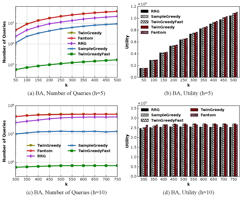
It can be easily verified that the social network monitoring problem considered in Section 5 is a non-monotone submodular maximization problem subject to a partition matroid constraint. We provide additional experimental results on Barabasi-Albert (BA) random graphs, as shown in Fig. 3. In Fig. 3, we generate a BA graph with 10,000 nodes and , and set for Fig. 3(a)-(b) and set for Fig. 3(c)-(d), respectively. The other settings in Fig. 3 are the same with those for ER random graph in Section 5. It can be seen that the experimental results in Fig. 3 are qualitatively similar to those on the ER random graph, and TwinGreedyFast still runs more than an order of magnitude faster than the other three algorithms. Besides, it is observed from Fig. 3 that TwinGreedyFast and TwinGreedy perform closely to Fantom and slightly outperform RRG and SampleGreedy on utility, while it is also possible that TwinGreedyFast/TwinGreedy can outperform Fantom on utility in some cases.
In Table 2, we study how the utility of TwinGreedyFast can be affected by the parameter . The experimental results in Table 2 reveal that, the utility of TwinGreedyFast slightly increases when decreases, and almost does not change when is sufficiently small (e.g., ). Therefore, we would not suffer a great loss on utility by setting to a relatively large number in for TwinGreedyFast.
| 50 | 100 | 150 | 200 | 250 | 300 | 350 | 400 | 450 | 500 | |
|---|---|---|---|---|---|---|---|---|---|---|
| 0.2 | 0.145 | 0.281 | 0.410 | 0.529 | 0.637 | 0.744 | 0.836 | 0.925 | 1.004 | 1.078 |
| 0.15 | 0.149 | 0.289 | 0.415 | 0.535 | 0.643 | 0.747 | 0.841 | 0.929 | 1.008 | 1.082 |
| 0.1 | 0.154 | 0.291 | 0.418 | 0.538 | 0.648 | 0.751 | 0.846 | 0.933 | 1.013 | 1.085 |
| 0.05 | 0.154 | 0.293 | 0.421 | 0.540 | 0.651 | 0.753 | 0.848 | 0.935 | 1.015 | 1.087 |
| 0.02 | 0.155 | 0.294 | 0.422 | 0.541 | 0.652 | 0.754 | 0.849 | 0.936 | 1.015 | 1.087 |
| 0.01 | 0.155 | 0.294 | 0.422 | 0.541 | 0.652 | 0.754 | 0.849 | 0.936 | 1.015 | 1.087 |
| 0.005 | 0.155 | 0.294 | 0.422 | 0.541 | 0.652 | 0.754 | 0.849 | 0.936 | 1.015 | 1.088 |
C.2 Multi-Product Viral Marketing
We first prove that the multi-product viral marketing application considered in Section 5 is an instance of the problem of non-monotone submodular maximization subject to a matroid constraint. Recall that we need to select seed nodes from a social network to promote products, and each node can be selected as a seed for at most one product. These requirements can be modeled as a matroid constraint, as proved in the following lemma:
Lemma 11
Define the ground set and , where for any . Then is a matroid.
Proof of Lemma 11: It is evident that is an independence system. Next, we prove that it satisfies the exchange property. For any and satisfying , there must exist certain such that (i.e., and ), because otherwise we have ; contradicting . As , we can add the element in into without violating the feasibility of , which proves that satisfies the exchange property of matroids.
Next, we prove that the objective function in multi-product viral marketing is a submodular function defined on :
Lemma 12
For any and , define
| (37) |
where and is a non-negative submodular function defined on (i.e., an influence spread function). We also define . Then is a submodular function defined on .
Proof of Lemma 12: For any and any , we must have and . So we get . If , then we have and hence due to and the submodularity of . If , then we also have , which completes the proof.
As we set , the objective function is also non-negative. Note that denotes the total expected number of nodes in that can be activated by under the celebrated Independent Cascade (IC) Model [34]. As evaluating for any given under the IC model is an NP-hard problem, we use the estimation method proposed in [7] to estimate , based on the concept of “Reverse Reachable Set” (RR-set). For completeness, we introduce this estimation method in the following:
Given a directed social network with each edge associated with a probability , a random RR-set under the IC model is generated by: (1) remove each edge independently with probability and reverse ’s direction if it is not removed; (2) sample uniformly at random and set as the set of nodes reachable from in the graph generated by the first step. Given a set of random RR-sets, any and any , we define
| (38) |
According to [7], is an unbiased estimation of , and is also a non-negative monotone submodular function defined on . Therefore, in our experiments, we generate a set of one million random RR-sets and use to replace in the objective function shown in Eqn. (37), which keeps as a non-negative submodular function defined on .