Deterministic Equations for Feedback Control of Open Quantum Systems

Introduction.— Feedback control finds numerous applications across practically all quantum coherent platforms, in tasks such as cooling protocols Hopkins et al. (2003); D’Urso et al. (2003); Steck et al. (2006); Bushev et al. (2006); Jacobs et al. (2015); Frimmer et al. (2016); Guo et al. (2019); Buffoni et al. (2019); Manikandan and Qvarfort (2023); De Sousa et al. (2025), quantum error correction Sarovar et al. (2004); Marcos et al. (2020), entanglement generation Ristè et al. (2013), thermodynamics Pekola (2015); Potts and Samuelsson (2018); Barker et al. (2022), transport van der Wiel et al. (2002), control Vijay et al. (2012); Ristè et al. (2012); Campagne-Ibarcq et al. (2013), and quantum batteries Mitchison et al. (2021). Notably, feedback has been instrumental in the experimental realization of Maxwell’s demon in the quantum regime Vidrighin et al. (2016); Naghiloo et al. (2018); Ribezzi-Crivellari and Ritort (2019), prompting the development of generalized formulations of the second law of thermodynamics to incorporate feedback-based measurement processes Sagawa and Ueda (2010, 2012); Funo et al. (2013). These developments highlight the fundamental importance of quantum feedback in both theory and experiment, motivating further research into its underlying principles and applications.

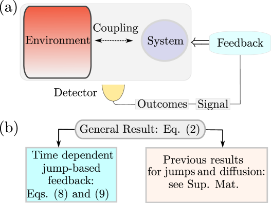
Broadly speaking, feedback refers to the process of dynamically controlling a system based on previous detection outcomes (see Fig. 1(a)). In continuously monitored open quantum systems this can be readily implemented using stochastic differential equations, both in the quantum jump and the quantum diffusion (e.g. homodyne/heterodyne) unravellings Belavkin (1983, 1992a, 1987, 1992b); Wiseman (1994a); Wiseman and Milburn (1993, 2010); Korotkov (2001); Jacobs (2014); Zhang et al. (2017). However, this approach typically requires computationally expensive statistical sampling and often obscures physical insights, as it does not yield analytical expressions for key system properties, such as the steady state (when it exists). For this reason, deterministic feedback equations have long been sought for Sarovar et al. (2004); Tilloy (2024); Annby-Andersson et al. (2022); Wiseman and Milburn (1993); Wiseman (1994b); Wiseman and Milburn (2010); Kewming et al. (2024).

Let $x_{1:n}=(x_{1},x_{2},\dots,x_{n})$ denote some stochastic data obtained from an experiment. Typically, feedback schemes do not make use of the entire dataset. Instead, they rely on a compressed representation of the data, which we henceforth refer to as the signal. This signal is defined as a function of the data, $y_{n}=y_{n}(x_{1:n})$. Hence, to classify different types of feedback schemes, it is helpful to clarify (i) what signal is being used and (ii) what the corresponding feedback actions are. For a given choice of signal, one can then construct various types of feedback actions. An illustrative example is homodyne detection-based feedback Wiseman and Milburn (1993): the data $x_{n}$ is the homodyne current; the signal is the instantaneous outcome ($y_{n}=x_{n}$); and the action is a drive in the system Hamiltonian $H(y_{n})$ that depends on the magnitude of the signal. Ref. Annby-Andersson et al. (2022) recently extended this to low-pass (LP) filters of the form $y_{n}=\sum_{i=1}^{n}\delta t\gamma e^{-\gamma\delta t(n-i)}x_{i}$, for a bandwidth $\gamma$. The particular case in which all detection weights are equal to one corresponds to a signal that depends on the entire history (often called the “integrated charge”), $y_{n}=\sum_{j=1}^{n}x_{j}$, and was studied in Kewming et al. (2024). In these cases, the authors derive deterministic equations that describe the feedback protocol based on the corresponding signals.

To further illustrate this point, Ref. Wiseman (1994a) derived a famous deterministic jump equation that implements the following protocol: if a quantum jump is observed, then we apply a quantum channel. The channel is now an abrupt action, that instantaneously modifies the system. Extending this to a smooth time-dependent action, such as turning on a Hamiltonian drive, is one of our present goals. Furthermore, for more general jump-based feedback — especially those involving time-dependent actions — no deterministic equations are typically available. For instance, in the case of quantum jumps, the output data $x_{n}$ at each time step $t_{n}=n\delta t$ is not a continuous, noisy current, but rather a discrete sequence of “clicks”, being either $x_{n}=0$ (no jump) or $x_{n}=k=1,2,\ldots$ for a jump in channel $k$. A natural kind of feedback for quantum jumps would be: if a quantum jump is observed, modify the Hamiltonian for some fixed amount of time. This protocol is, in fact, routinely used in quantum dot experiments which monitor the jumps using a quantum point contact Hofmann et al. (2016); Ye et al. (2025). However, this cannot be described using only feedback based on the latest outcome ($y_{n}=x_{n}$) because most of the time we would have $y_{n}=0$. Consequently, feedback schemes that depend on jump timing generally lack a corresponding deterministic evolution equation.

In this letter we consider the most general type of continuously monitored open quantum system, formulated in terms of quantum instruments Milz and Modi (2021). We first show (Result 1) that it is possible to derive a deterministic feedback equation for any signal that can be written as $y_{n}=f_{n}(x_{n},y_{n-1})$, where $f_{n}$ is an update rule that depends only on the previous signal and the present outcome. To illustrate the generality and power of this result, in the Supplemental Material Sup we use it to derive various other deterministic feedback equations Annby-Andersson et al. (2022); Wiseman and Milburn (1993); Wiseman (1994b); Kewming et al. (2024) in the literature (see Fig. 1(b)). Next, we specialize this to the case of quantum jumps, and derive a deterministic equation (Result 2) that allows for feedback based on: (i) what was the channel of the last jump [Eq. (6)] and (ii) how long has it been since the last jump occurred [Eq. (7)]. The combination of these two features allow for non-trivial feedback strategies that are experimentally relevant Hofmann et al. (2016); Ye et al. (2025). For example, one can turn on coherent drives based on whether a tunneling event into or out of a quantum dot has occurred, or depending on whether a photon has been emitted or absorbed by an atom. More sophisticated strategies are also possible, such as turning on a drive only after a certain time has elapsed since the last detected jump.

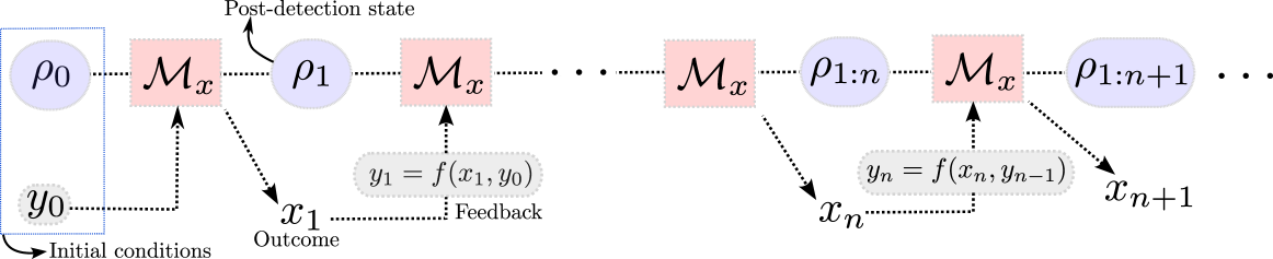
Sequential measurements.$-$ Continuously measured quantum systems can be described by the sequential application of super-operators $\{\mathcal{M}_{x}\}$, corresponding to trace non-increasing maps such that $\sum_{x}\mathcal{M}_{x}$ is a quantum channel Milz and Modi (2021). These maps are called instruments, and they describe the joint transition of the quantum state induced by the dynamical evolution and measurement process, whereas $x$ represents a possible measurement outcome.

For instance, one may assume that the measurements are described by the set $\{V_{x}\}$ of Kraus operators applied at regular intervals $t_{j}=j\delta t$, where $j=0,1,2,\dots$ and $\delta t>0$. In between, the system may evolve from $t$ to $t+\delta t$ with some dynamical map $\rho(t+\delta t)=\Lambda_{t+\delta t,t}\rho(t)$. Given an initial state $\rho_{0}$, after $n$ steps one obtains a sequence of outcomes $x_{1:n}=(x_{1},x_{2},\dots,x_{n})$, and the corresponding conditional state of the system is denoted by $\rho_{1:n}$. In this case, the instruments are defined as the maps $\mathcal{M}_{x}\rho=V_{x}[\Lambda_{t+\delta t,t}(\rho)]V_{x}^{\dagger}$, and according to the measurement postulate, the probability of the next outcome $x_{n+1}$ given the previous dataset $x_{1:n}$ is given by $P(x_{n+1}|x_{1:n})=\mathrm{Tr}[\mathcal{M}_{x_{n+1}}(\rho_{x_{1:n}})]$, and the post-detection state becomes $\rho_{x_{1:n+1}}=\frac{\mathcal{M}_{x_{n+1}}(\rho_{x_{1:n}})}{P(x_{n+1}|x_{1:n})}$.

A feedback mechanism is a dynamic adjustment of the instruments $\mathcal{M}_{x}$ at each step, based on prior outcomes. The most general mechanism could depend on the entire detection history, and would therefore give rise to instruments of the form $\mathcal{M}_{x_{n}}(x_{1:n-1})$, where the variable in the subscript defines the possible random outcomes and the variable in parenthesis defines the past information that can be used to alter the instrument. In practice, however, one seldom uses the entire data record $x_{1:n}$, but only some summary statistic. Here we implement this by defining a signal $y_{n}$ which evolves according to the update rule $y_{n}=f_{n}(x_{n},y_{n-1})$, for some function $f_{n}$. This defines a general type of causal signal. But it is worth noting that this is still entirely general. For instance, if we choose an update rule of the form $y_{n}=\text{append}(y_{n-1},x_{n})$, then the signal becomes the entire dataset. But, of course, in this case the memory required grows with each step. In practice, however, one is often interested in signals with finite memory. Feedback is implemented by assuming that, in each step, the instruments can depend on the signal at that instant (see Fig. 2). The stochastic dynamics therefore reads

Our goal is to develop a deterministic equation for this general feedback protocol. To do that we define the signal-resolved state Kewming et al. (2024); Annby-Andersson et al. (2022) (also called Hybrid Quantum-Classical State Tilloy (2024); Layton et al. (2024); Diósi (2023); Oppenheim et al. (2023)) as $\varrho_{n}(y)=E[\rho_{1:n}\delta_{y,y_{n}}]$, where $E[\cdot]$ denotes the average over trajectories, and $\delta_{y,y_{n}}$ is the Kronecker delta. The trace of this state, $\mathrm{Tr}[\varrho_{n}(y)]=P(y_{n}=y)$, gives the distribution of the stochastic signal at step $n$, while the marginalization over all possible signals yields the unconditional state of the system, $\sum_{y}\varrho_{n}(y)=\bar{\rho}_{n}$. Notice that $\rho_{x_{1:n}}$ is a stochastic (conditional) state, but $\varrho_{n}(y)$ is deterministic. As our first result, we show in Sup that $\varrho_{n}(y)$ evolves according to a deterministic equation.

The particular case $y_{n}=x_{n}$ is treated separately in Sup , section S.V.B. The intuition behind (2) is that because $\varrho_{n}(y)$ is resolved in $y$, the state at step $n+1$ should be just a sum over all possible trajectories consistent with the constraint $y_{n}=f_{n}(x_{n},y_{n-1})$. Solving (2) yields not only the unconditional state $\bar{\rho}_{n}$, but also the probability distribution $P(y_{n}=y)$ of the stochastic signal $y_{n}$. Moreover, it can be used to study either transients or the steady-state, obtained by setting $\varrho_{n+1}(y)=\varrho_{n}(y)=\varrho_{\rm ss}(y)$. To illustrate the generality of this result, in Sup we use it to derive various other deterministic equations in the literature Annby-Andersson et al. (2022); Wiseman and Milburn (1993); Wiseman (1994b); Kewming et al. (2024).

Quantum jumps.$-$ We now specialize Result 1 to the case of quantum jumps, for which deterministic feedback equations are much more scarce. We assume the system evolves according to a quantum master equation of the form

with Hamiltonian $H$ and jump operators $L_{k}$. Our goal is to augment this with the possibility that $H(y)$ and $\{L_{k}(y)\}$ both depend on the recorded signal $y$.

Let $\Sigma$ denote the set of jumps that are assumed to be monitored. At the stochastic level, the outcome at each step $\delta t$ is either $x_{n}=0$ (no jump) or $x_{n}=k\in\Sigma$ when there is a jump of type $k$. The corresponding instruments read Landi et al. (2024)

where $\mathcal{J}_{k}(y)\rho=L_{k}(y)\rho L_{k}^{\dagger}(y)$ and $\mathcal{L}_{0}(y)=\mathcal{L}(y)-\sum_{k\in\Sigma}\mathcal{J}_{k}(y)$.

We consider two types of signals. First, one that records the channel $k\in\Sigma$ of the last jump. This can be constructed with a filter function $f_{n}$ of the form

Second, a signal that counts how much time has elapsed since the last jump, which is built using

We refer to them as the jump signal and the counting signal, respectively. The total signal is $y_{n}=(k_{n},\tau_{n})$ and we consider feedback mechanisms that may depend on both. In this case, the instruments are defined by Eqs. (4) and (5), and the feedback action corresponds to allowing both the system’s Hamiltonian $H$ and the jump operators $L_{k}$ at step $n$ to depend on the last jump $k_{n-1}$ and the elapsed time $\tau_{n-1}$ since its detection. Starting from Result 1, we show in Sup the following result:

In this limit $\delta t\to 0$ the signals become continuous-time stochastic processes $k_{t}$ and $\tau_{t}$. They specify that, at time $t$, the last jump that happened was in channel $k_{t}$, and occurred at time $t-\tau_{t}$. The quantity $\mathrm{Tr}[\varrho_{t}(k,\tau)]$ is the joint distribution of $(k_{t},\tau_{t})$, and from (7) it follows that $\tau_{t}\in[0,t]$. The resolved state is normalized as $\sum_{k\in\Sigma}\int_{0}^{t}\mathrm{Tr}[\varrho_{t}(k,\tau)]d\tau=1$, and the unconditional state is recovered as

Result 2 cannot, in general, be written as a differential equation. Notwithstanding, it is still amenable to analytical treatment — as detailed in Sup — especially if one is interested in the steady-state. In contrast, let us now consider the special case where the feedback is independent of the counting signal (7), but might still depend on the jump signal (6). We show in Sup that the marginal state $\varrho_{t}(k)=\int_{0}^{t}d\tau\varrho_{t}(k,\tau)$ will evolve as

This is now simply a system of coupled master equations, one for each possible jump channel $k\in\Sigma$. A similar equation was previously derived in Blanchard and Jadczyk (1995) in a different context.

Returning to the general Result 2, the situation simplifies when the feedback is applied only on the no-jump part of the dynamics (e.g. in the Hamiltonian). In this case $\mathcal{J}_{k}(k^{\prime},\tau^{\prime})=\mathcal{J}_{k}$ and Eqs. (8)- (10) imply that

The signal-resolved state can hence be written in terms of the unconditional state $\bar{\rho}_{t}$ which, in turn, satisfies the closed integral equation

The steady-state, if it exists, is obtained by setting $t\to\infty$ and will therefore be the solution of the algebraic equation

Combining this with Eq. (12) yields the steady-state signal-resolved state. In turn, this can be used to calculate various time-related properties, such as waiting-time distributions, the average time between jumps, etc.

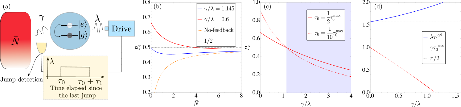
Example.– To illustrate our results, consider a coherently driven qubit coupled to a thermal reservoir with temperature $T$ and energy $\omega$ under the action of feedback. Let $\ket{e}$ (excited) and $\ket{g}$ (ground) denote the computational basis. We assume a master equation of the form (3) with jump operators $L_{-}=\sqrt{\gamma(\bar{N}+1)}\leavevmode\nobreak\ |g\rangle\langle e|$ and $L_{+}=\sqrt{\gamma\bar{N}}\leavevmode\nobreak\ |e\rangle\langle g|$ describing, respectively, the emission and absorption of a quanta. Here $\bar{N}=(\text{exp}(\omega/T)-1)^{-1}$ is the Bose-Einstein distribution and $\gamma>0$ is the coupling strength. The 3 possible outcomes, at each $dt$, are therefore $x_{n}=-1,+1,0$ (emission, absorption, no-jump). We consider a drive with intensity $\lambda$ and frequency $\omega_{d}$, working in a frame rotating at $\omega_{d}$ and under the rotating wave approximation. The Hamiltonian when the driving is turned off/on are, respectively, $H_{\text{off}}=-\frac{\Delta}{2}\sigma_{z}$ and $H_{\text{on}}=-\frac{\Delta}{2}\sigma_{z}+\lambda\sigma_{x}$, where $\Delta=\omega-\omega_{d}$. Our goal is to invert the populations of $\ket{e}$ and $\ket{g}$ (achieving $P_{e}>P_{g}$) using the quantum jump detection record and feedback.

The protocol is defined as follows: If $x_{n}=+1$ (thermal absorption) the system’s Hamiltonian is set to $H=H_{\text{off}}$. If $x_{n}=-1$ (thermal emission), and a time $\tau_{0}$ elapses without any subsequent absorption, we turn the external drive ($H=H_{\text{on}}$) for a duration $\tau_{1}$. The idea is that, upon detecting an emission and observing no absorption for a time $\tau_{0}$, the external drive acts on the system for a time $\tau_{1}$, inducing Rabi oscillations that transfer the population from $\ket{g}$ to $\ket{e}$ (see Fig. 3(a)). Whenever the drive is active and an absorption event is detected, the drive is subsequently turned off.

This feedback protocol affects only the system’s Hamiltonian; hence, the steady state can be obtained from Eq. (14). The analytical formula for the population of the excited state, $P_{e}\equiv\left<e|\rho_{ss}|e\right>$, is provided Sup for the case $\Delta=0$, as a function of the bath parameters $\bar{N}$ and $\gamma$, as well as the feedback parameters $\lambda$, $\tau_{0}$, and $\tau_{1}$. By maximizing $P_{e}$ with respect to $\tau_{1}$, one obtains the optimal duration $\tau_{1}^{\text{opt}}$ for which the external drive should remain on. We find that

where $p=\gamma/\lambda$ and $\theta(x)$ is the Heaviside function. This is only finite for $p<4$, and diverges otherwise. It is noteworthy that $\tau_{1}^{\text{opt}}$ is independent of both the feedback delay $\tau_{0}$ and the bath occupation $\bar{N}$; it depends only the ratio $p=\gamma/\lambda$ between the coupling rate to the bath and the external drive. Fig. 3(b) shows $P_{e}$ vs. $\bar{N}$ for $\tau_{0}=0$. We find that for $\gamma/\lambda\leq 1.145$ (determined numerically), there exists a critical value $\bar{N}_{\text{c}}\geq 0$ such that $P_{e}>1/2$ for all $\bar{N}<\bar{N}_{\text{c}}$. This therefore establishes the population inversion threshold. For $\gamma/\lambda>1.145$ the drive is so weak that a pi pulse takes a time that is longer than the time-scale over which the bath exchanges energy with the qubit.

Next we consider a more realistic scenario where we have a time delay $\tau_{0}$ between the last detected jump $x_{n}=-1$ and the moment the external drive is turned on. Even in this more general case, the optimal drive duration that maximizes the population of the excited state remains given by Eq. (15) Sup . In the low-temperature limit $\bar{N}\rightarrow 0$, the expression for $P_{e}$, evaluated at the optimal drive duration, simplifies to

The time delay appear as an additive term $\gamma\leavevmode\nobreak\ \tau_{0}$ in the denominator. The largest delay that still provides a population inversion ($P_{e}=1/2$) in the low-temperature limit ($\bar{N}\rightarrow 0$) is

In Fig. 3(c), we illustrate how $P_{e}$ is affected by varying the delay $\tau_{0}$. We consider $\bar{N}=0$, for which $P_{e}=1/2$ occurs precisely at $\gamma/\lambda=1.145$. The plots show how increasing $\tau_{0}$ deteriorates the population inversion. Fig. 3(d) plots Eqs. (15) and (17) vs. $\gamma/\lambda$, again for $\bar{N}=0$. In the strong-drive regime ($\gamma\ll\lambda$), we find that $\tau_{0}^{\text{max}}\sim 1/\gamma$, indicating that the maximum delay is on the order of the system’s natural timescale $\gamma^{-1}$. Conversely, $\tau_{0}^{\text{max}}=0$ for $\gamma/\lambda>1.145$, reflecting that population inversion is no longer possible in this regime, regardless of the feedback delay. Additionally, we observe that $\gamma\tau_{1}^{\text{opt}}$ increases with $\gamma/\lambda$, implying that as the drive strength $\lambda$ decreases relative to $\gamma$, the drive must remain on for a longer duration to optimize $P_{e}$.

As a final comment, it is worth mentioning that this protocol can be adapted to increase the population of the ground state: by turning on the drive when an absorption is detected, the drive will move the system toward the ground state through Rabi oscillations. In this case, the protocol effectively operates as a cooling protocol based on quantum jump detections.

Conclusion.—We derived a deterministic equation that describes a general feedback protocol, encompassing both discrete and continuous feedback. It encompass previous results as particular cases, and allows for the derivation of novel feedback schemes, as we have shown here in the context of quantum jumps. The method is based on a signal-resolved state, which provides access not only to the quantum dynamics, but also to the full statistics of the detection signal. Furthermore, it is a deterministic approach, which introduces new analytical tools that offer deeper physical insight into the interplay between feedback and quantum dynamics. Its applications span a wide range of fields, with particular relevance to quantum control, thermodynamics, and quantum information theory. We illustrated this with a detailed account of the use quantum jump detections and feedback for population inversion of a two-level system.

Acknowledgments.— The authors acknowledge fruitful discussions with Mark Mitchison, Guilherme Fiusa, Abhaya Hegde.

References

- Hopkins et al. (2003) A. Hopkins, K. Jacobs, S. Habib, and K. Schwab, Phys. Rev. B 68, 235328 (2003).
- D’Urso et al. (2003) B. D’Urso, B. Odom, and G. Gabrielse, Phys. Rev. Lett. 90, 043001 (2003).
- Steck et al. (2006) D. A. Steck, K. Jacobs, H. Mabuchi, S. Habib, and T. Bhattacharya, Phys. Rev. A 74, 012322 (2006).
- Bushev et al. (2006) P. Bushev, D. Rotter, A. Wilson, F. m. c. Dubin, C. Becher, J. Eschner, R. Blatt, V. Steixner, P. Rabl, and P. Zoller, Phys. Rev. Lett. 96, 043003 (2006).
- Jacobs et al. (2015) K. Jacobs, H. I. Nurdin, F. W. Strauch, and M. James, Phys. Rev. A 91, 043812 (2015).
- Frimmer et al. (2016) M. Frimmer, J. Gieseler, and L. Novotny, Phys. Rev. Lett. 117, 163601 (2016).
- Guo et al. (2019) J. Guo, R. Norte, and S. Gröblacher, Phys. Rev. Lett. 123, 223602 (2019).
- Buffoni et al. (2019) L. Buffoni, A. Solfanelli, P. Verrucchi, A. Cuccoli, and M. Campisi, Phys. Rev. Lett. 122, 070603 (2019).
- Manikandan and Qvarfort (2023) S. K. Manikandan and S. Qvarfort, Phys. Rev. A 107, 023516 (2023).
- De Sousa et al. (2025) G. De Sousa, P. Bakhshinezhad, B. Annby-Andersson, P. Samuelsson, P. P. Potts, and C. Jarzynski, Phys. Rev. E 111, 014152 (2025).
- Sarovar et al. (2004) M. Sarovar, C. Ahn, K. Jacobs, and G. J. Milburn, Phys. Rev. A 69, 052324 (2004).
- Marcos et al. (2020) D. Marcos, A. Smith, A. Bednorz, and N. Yunger Halpern, Phys. Rev. X 10, 041013 (2020).
- Ristè et al. (2013) D. Ristè, M. Dukalski, C. A. Watson, G. de Lange, M. J. Tiggelman, Y. M. Blanter, K. W. Lehnert, R. N. Schouten, and L. DiCarlo, Nature 502, 350 (2013).
- Pekola (2015) J. P. Pekola, Nature Physics 11, 118 (2015).
- Potts and Samuelsson (2018) P. P. Potts and P. Samuelsson, Phys. Rev. Lett. 121, 210603 (2018).
- Barker et al. (2022) D. Barker, M. Scandi, S. Lehmann, C. Thelander, K. A. Dick, M. Perarnau-Llobet, and V. F. Maisi, Phys. Rev. Lett. 128, 040602 (2022).
- van der Wiel et al. (2002) W. G. van der Wiel, S. De Franceschi, J. M. Elzerman, T. Fujisawa, S. Tarucha, and L. P. Kouwenhoven, Rev. Mod. Phys. 75, 1 (2002).
- Vijay et al. (2012) R. Vijay, C. Macklin, D. H. Slichter, S. J. Weber, K. W. Murch, R. Naik, A. N. Korotkov, and I. Siddiqi, Nature 490, 77 (2012).
- Ristè et al. (2012) D. Ristè, C. C. Bultink, K. W. Lehnert, and L. DiCarlo, Phys. Rev. Lett. 109, 240502 (2012).
- Campagne-Ibarcq et al. (2013) P. Campagne-Ibarcq, E. Flurin, N. Roch, D. Darson, P. Morfin, M. Mirrahimi, M. H. Devoret, F. Mallet, and B. Huard, Phys. Rev. X 3, 021008 (2013).
- Mitchison et al. (2021) M. T. Mitchison, J. Goold, and J. Prior, Quantum 5, 500 (2021).
- Vidrighin et al. (2016) M. D. Vidrighin, O. Dahlsten, M. Barbieri, M. S. Kim, V. Vedral, and I. A. Walmsley, Phys. Rev. Lett. 116, 050401 (2016).
- Naghiloo et al. (2018) M. Naghiloo, J. J. Alonso, A. Romito, E. Lutz, and K. W. Murch, Phys. Rev. Lett. 121, 030604 (2018).
- Ribezzi-Crivellari and Ritort (2019) M. Ribezzi-Crivellari and F. Ritort, Nature Physics 15, 660 (2019).
- Sagawa and Ueda (2010) T. Sagawa and M. Ueda, Phys. Rev. Lett. 104, 090602 (2010).
- Sagawa and Ueda (2012) T. Sagawa and M. Ueda, Phys. Rev. Lett. 109, 180602 (2012).
- Funo et al. (2013) K. Funo, Y. Watanabe, and M. Ueda, Phys. Rev. E 88, 052121 (2013).
- Belavkin (1983) V. P. Belavkin, Autom. Remote Control 44, 178 (1983).
- Belavkin (1992a) V. P. Belavkin, J. Multivar. Anal. 42, 171 (1992a).
- Belavkin (1987) V. P. Belavkin, in Information Complexity and Control in Quantum Physics, edited by A. Blaquiere, S. Diner, and G. Lochak (Springer Vienna, Vienna, 1987) pp. 311–329.
- Belavkin (1992b) V. P. Belavkin, Commun. Math. Phys. 146, 611 (1992b).
- Wiseman (1994a) H. M. Wiseman, Phys. Rev. A 49, 2133 (1994a).
- Wiseman and Milburn (1993) H. M. Wiseman and G. J. Milburn, Phys. Rev. Lett. 70, 548 (1993).
- Wiseman and Milburn (2010) H. M. Wiseman and G. J. Milburn, Quantum Measurement and Control (Cambridge University Press, 2010).
- Korotkov (2001) A. N. Korotkov, Phys. Rev. B 63, 115403 (2001).
- Jacobs (2014) K. Jacobs, Quantum Measurement Theory and Its Applications (Cambridge University Press, 2014).
- Zhang et al. (2017) J. Zhang, Y.-X. Liu, R.-B. Wu, K. Jacobs, and F. Nori, Phys. Rep. 679, 1 (2017).
- Tilloy (2024) A. Tilloy, SciPost Phys. 17, 083 (2024).
- Annby-Andersson et al. (2022) B. Annby-Andersson, F. Bakhshinezhad, D. Bhattacharyya, G. De Sousa, C. Jarzynski, P. Samuelsson, and P. P. Potts, Phys. Rev. Lett. 129, 050401 (2022).
- Wiseman (1994b) H. M. Wiseman, Phys. Rev. A 49, 2133 (1994b).
- Kewming et al. (2024) M. J. Kewming, A. Kiely, S. Campbell, and G. T. Landi, Phys. Rev. A 109, L050202 (2024).
- (42) See the Supplemental Material at [URL will be inserted by publisher] for details.
- Hofmann et al. (2016) A. Hofmann, V. F. Maisi, C. Gold, T. Krähenmann, C. Rössler, J. Basset, P. Märki, C. Reichl, W. Wegscheider, K. Ensslin, and T. Ihn, Phys. Rev. Lett. 117, 206803 (2016).
- Ye et al. (2025) F. Ye, A. Ellaboudy, and J. M. Nichol, Phys. Rev. Appl. 23, 044063 (2025).
- Milz and Modi (2021) S. Milz and K. Modi, PRX Quantum 2, 030201 (2021).
- Layton et al. (2024) I. Layton, J. Oppenheim, and Z. Weller-Davies, Quantum 8, 1565 (2024).
- Diósi (2023) L. Diósi, Phys. Rev. A 107, 062206 (2023).
- Oppenheim et al. (2023) J. Oppenheim, C. Sparaciari, B. Šoda, and Z. Weller-Davies, Quantum 7, 891 (2023).
- Landi et al. (2024) G. T. Landi, M. J. Kewming, M. T. Mitchison, and P. P. Potts, PRX Quantum 5, 020201 (2024).
- Blanchard and Jadczyk (1995) P. Blanchard and A. Jadczyk, Annalen der Physik 507, 583 (1995).
- Oppenheim (2023) J. Oppenheim, Phys. Rev. X 13, 041040 (2023).
- Jacobs and Steck (2006) K. Jacobs and D. A. Steck, Contemporary Physics 47, 279 (2006).
- Bednorz et al. (2012) A. Bednorz, W. Belzig, and A. Nitzan, New Journal of Physics 14, 013009 (2012).
Appendix A Supplementary Material
We begin by introducing the language of instruments in Section B, defining the concepts that were used throughout this work. Next, we provide a detailed proof of the central results presented in the main text – namely, Results 1 and 2 – in Section C. Furthermore, we present a formulation in terms of matrix equations for the main results in Section D, where we also include a discussion about the steady state and generator of the feedback dynamics. In Section E, we present the details of the example used in the main text, namely the inversion protocol, and finally in Section F we show how some previous results can be recovered starting from Eq. (18).