Deterministic Lower Bounds for -Edge Connectivity in the Distributed Sketching Model
Abstract
We study the -edge connectivity problem on undirected graphs in the distributed sketching model, where we have nodes and a referee. Each node sends a single message to the referee based on its 1-hop neighborhood in the graph, and the referee must decide whether the graph is -edge connected by taking into account the received messages.
We present the first lower bound for deciding a graph connectivity problem in this model with a deterministic algorithm. Concretely, we show that the worst case message length is bits for -edge connectivity, for any super-constant . Previously, only a lower bound of bits was known for (-edge) connectivity, due to Yu (SODA 2021). In fact, our result is the first super-polylogarithmic lower bound for a connectivity decision problem in the distributed graph sketching model.
To obtain our result, we introduce a new lower bound graph construction, as well as a new 3-party communication complexity problem that we call . As this problem does not appear to be amenable to reductions to existing hard problems such as set disjointness or indexing due to correlations between the inputs of the three players, we leverage results from cross-intersecting set families to prove the hardness of for deterministic algorithms. Finally, we obtain the sought lower bound for deciding -edge connectivity via a novel simulation argument that, in contrast to previous works, does not introduce any probability of error and thus works for deterministic algorithms.
1 Introduction
We consider the distributed graph sketching model [BMN+11], where distributed nodes each observe their list of neighbors in a graph. Every node sends a single message to a central entity, called referee, who must compute a function of the graph based on the received messages. In this setting, any graph problem can be solved trivially by instructing each one of the nodes to simply include their entire neighborhood information in the message to the referee. To obtain more efficient algorithms that scale to large graphs, the main goal is to keep the maximum size of these messages (also called sketches) as small as possible, preferably polylogarithmic in . In contrast, the full list of neighbors of a node could be as large as bits, under the standard assumption that the node IDs are a permutation of . Consequently, nodes can afford to convey only incomplete information (hence the name “sketch”) of their local neighbors to the referee, which may paint a somewhat ambiguous picture of the actual graph. While it may be tempting to conclude that small sketches do not allow us to solve interesting graph problems in this model, the surprising breakthrough of Ahn, Guha, and McGregor [AGM12a] showed that several fundamental graph problems, such as connectivity and spanning trees, can indeed be solved with sketches of only bits, if nodes have access to shared randomness and one is willing to accept a polynomially small probability of error. Their technique (called “AGM sketches”) paved the way for sketch-based graph algorithms for many other graph problems, including vertex connectivity [GMT15] and approximate graph cuts [AGM12b]; see the survey of [McG14] for a list of additional graph problems.111Strictly speaking, [AGM12a] showed these results for fully dynamic graph streams in the semi-streaming model, but it is straightforward to adapt them to the distributed graph sketching model, as observed in [BMRT14].
1.1 Randomized Lower Bounds for Connectivity Problems
The question whether AGM sketches are optimal for connectivity problems remained an open problem for several years, until the seminal work by Nelson and Yu [NY19] showed that bits are indeed required for computing spanning forests in the distributed graph sketching model. The main idea of their lower bound is to use a reduction to a variant of the universal relation problem [KRW95] in 2-party communication complexity, denoted by , where Alice starts with a subset of some universe , and Bob gets a proper subset . Alice sends a single message to Bob, who must output some element in . In [KNP+17a], Kapralov, Nelson, Pachoki, Wang, and Woodruf showed that bits are required for solving with high probability. To obtain a reduction to in the distributed sketching model, [NY19] define a tripartite graph on vertex sets , , and a much smaller set . Each node has a set of unique neighbors in (not shared with any other node in ) as well as some neighbors in . Since every node in is connected to at most one node , any spanning forest must include some edge between and a node in . The neighborhood of a randomly chosen is determined by the input of such that Alice’s set corresponds to all of ’s neighbors, whereby Bob’s set specifies the subset of neighbors in . They show that the players can jointly simulate the nodes in and (but not !), whereby Bob also simulates the referee. From the resulting spanning forest, Bob can extract an edge between and , which corresponds to an element in , and thus solves . Notably absent in their simulation are the nodes in , which neither Alice or Bob can simulate, due to their lack of knowledge of set . In fact, trying to faithfully simulate every node executing a distributed sketching algorithm in a 2-party model poses a major technical challenge since every edge is shared between its neighbors. However, [NY19] show that choosing to be polynomially smaller than suffices to overcome this obstacle: Since each will be a neighbor of many and does not know which of them is the important node (as all of these neighborhoods are sampled from the same hard input distribution for ), it follows that the amount of information that the referee can learn about the neighbors of from the sketches of the nodes in is only (roughly) , and thus negligible. Hence, Alice and Bob can omit these messages in their simulation altogether, while only causing a small increase in the overall error probability, due to Pinsker’s inequality [Pin64]. We remark that the actual lower bound construction of [NY19] uses multiple copies of this basic building block.
More recently, Robinson [Rob23] extended the approach of [NY19] to constructing a -edge connected spanning subgraph (-ECSS), with the main difference being a modified graph construction that enables a reduction to the multi-output variant of universal relation, called , which has a lower bound of bits [KNP+17a] and requires Bob to find elements of . The simulation argument in [Rob23] does not directly use Pinsker’s inequality as in [NY19], and instead obtains a slightly smaller, but nevertheless nonzero, probability of error, by devising a mechanism of reconstructing the output when omitting the sketches of the nodes in . At the risk of stating the obvious, we point out that this result does not have any implications for the problem of deciding whether a given graph is -edge connected, which is the focus of the current paper.
In [Yu21], Yu proved that the decision problem of graph connectivity is subject to the same lower bound on the message length as computing a spanning forest, which fully resolved the complexity of connectivity in the distributed sketching model. For this purpose, [Yu21] introduced and proved the hardness of a new decision version of universal relation, called . Just as for the problem, Alice again gets a set . However, Bob not only gets but, in addition, he also knows a partition of . The inputs adhere to the promise that either or , and, upon receiving Alice’s message, Bob needs to decide which is the case. In order to embed an instance of in a graph, [Yu21] adapted the construction of [NY19] by partitioning the set into and , and by sampling the neighborhood of each node in according to the hard distribution of . Following the overall simulation approach of [NY19], Alice’s input of is embedded at some special node . Accordingly, the partition-promise of translates to each having all its -neighbors in either or .
We point out that there does not appear to be a natural extension of the connectivity lower bound of [Yu21] to -edge connectivity. Even though can be generalized to , proving a lower bound that scales linearly with for this generalization appears to be far from straightforward. Interestingly, the situation is reversed for the standard “search” version of , where the proof of the lower bound for is technically less involved than the corresponding result for , see [KNP+17a]. A second obstacle is that, in contrast to the problem of finding a -edge connected spanning subgraph [Rob23], designing a suitable lower bound graph for deciding -edge connectivity is itself nontrivial. This is because choosing the neighborhood of every node in according to the hard distribution of the generalized variant of and embedding it in the constructions of [NY19, Yu21] may result in a graph that is very likely to be -edge connected, independently of the neighborhood of the special node .
1.2 Why Deterministic Lower Bounds?
Interestingly, none of the above mentioned lower bound results provide a straightforward way towards obtaining stronger bounds for deterministic graph sketching algorithms (that never fail): Since any deterministic one-way algorithm for , , or needs to send Alice’s entire input to Bob,222While there is no published deterministic lower bound for , the same communication complexity bound as for the search version follows from standard fooling set and counting arguments for one-way communication; see, e.g., [KN97]. it may appear that, at first glance, we can simply “plug in” these results for deterministic protocols and directly obtain stronger lower bounds in the graph sketching model. This intuition, however, turns out to be misleading, as a major technical challenge is that the simulations used in [NY19, Yu21, Rob23] are themselves randomized and, more importantly, are necessarily “lossy” in the sense that they introduce a nonzero probability of error, due to forgoing the simulation of some nodes—in particular, all nodes in . This poses a major technical obstacle towards obtaining lower bounds for algorithms that fail with exponentially small probability, including deterministic ones.333We discuss prior work on lower bounds for other graph problems in the sketching model in Section 1.4. To the best of our knowledge, achieving a perfect (i.e., -error) simulation of graph sketching algorithms in a two-party communication complexity model remains a challenging open problem.
1.3 Our Contributions
In this work, we take the first step toward determining lower bounds for deterministic connectivity algorithms in the graph sketching model. In more detail, we focus on the problem of deciding -edge connectivity, and we show that any deterministic sketching algorithm has a worst case sketch length that is almost linear (in ):
Theorem 1.
Every deterministic algorithm that decides -edge connectivity on -node graphs in the distributed sketching model has a worst case message length of bits, for any super-constant , where is a suitable constant.
The proof of Theorem 1 requires us to overcome several technical challenges:
-
•
To obtain a graph that is hard for deciding -edge connectivity in the distributed sketching model, we need to find a suitable graph construction. We cannot directly extend the constructions used for deciding graph connectivity in [Yu21], as this crucially rests on the assumption that the neighborhood of every node in (see Sec. 1.1) must be chosen from the same distribution. In fact, the straightforward generalization of this idea to -edge connectivity would yield a graph that is very likely to be -edge connected, for large values of . In this work, we propose a new construction that does not preserve the uniformity property of [Yu21] regarding the input distribution. Instead, there is a special node , with a somewhat larger degree than its peers, which we connect in a way such that the -edge connectivity of the graph entirely rests on the choice of neighborhood for this node. Nevertheless, we ensure that its neighbors have no easy way of distinguishing from the vast majority of unimportant nodes. This approach introduces additional technical difficulties that we address in our simulation.
-
•
As elaborated in more detail in Section 1.2, we need to depart from the well-trodden path of using the “partial simulation” argument pioneered in [NY19] (and also used in the work of [Yu21] and [Rob23]), where some nodes are omitted from being simulated, as this would result in a nonzero error algorithm. To avoid this pitfall, we design a completely different simulation that is suitable for deterministic algorithms. We point out that the main technical difficulty of the distributed sketching model, namely the “sharing” of edges between nodes, also surfaces in our setting and prevents us from devising a simulation, where every node ’s neighborhood is part of the input of one of the simulating players. Instead, we exploit some structural properties of the algorithm at hand that must hold for any deterministic protocol. In more detail, the main idea behind our approach is that it suffices to compute a sketch for that looks “compatible” with our (limited) knowledge of ’s neighborhood, and we prove that this indeed ensures an error free simulation.
-
•
Our simulation works in a simultaneous 3-party model of communication complexity, where two players, Alice and Bob, each send a single message to Charlie who computes the output. For this setting, we introduce the problem, which abstracts the core difficulty present in our lower bound graph construction: That is, nodes are unaware which of their incident edges point to the crucial node , even though itself is aware of its special role. We capture this property in the communication complexity setting by equipping Alice and Bob each with an input vector that has a single common coordinate whose XOR is . While Charlie knows the location of this coordinate, he does not know the values of the respective bits of Alice and Bob, which are needed for the correct output. The hardness of does not appear to follow from reductions to standard problems such as set disjointness or variants of indexing (see Sec. 4.1 for a more detailed discussion), due to the correlation between the inputs of the three players and since we consider ternary input vectors, whose entries may be either , , or . A further complication is that we need to assume Charlie knows the entire support (i.e., the indices of all non- entries) of Alice’s and Bob’s inputs. Instead, we devise a purely combinatorial argument based on properties of cross-intersecting set families to show the following result:
Theorem 2.
For any sufficiently large , there exists an such that the deterministic one-way communication complexity of in the simultaneous 3-party model is , where each -length input vector has support .
1.4 Additional Related Work
The distributed graph sketching model was first introduced by Becker, Matamala, Nisse, Rapaport, Suchan, and Todinca in [BMN+11], where they proved the hardness of several fundamental graph problems for deterministic sketching algorithms: In particular, they showed that problems including deciding whether the diameter is at most , and whether the graph contains a certain subgraph such as a triangle or a square, require sketches of large (i.e., super-polylogarithmic) size. Their approach works by showing that the existence of an efficient protocol for any of these problems can be leveraged for reconstructing graphs with certain properties using similar-sized sketches. However, as pointed out in [BMN+11], their approach does not extend to graph connectivity problems.
The model was further explored by Becker, Montealegre, Rapaport, and Todinca in [BMRT14], where they show separations between the power of deterministic, private randomness and public randomness algorithms. Apart from the aforementioned works of [NY19, Yu21, Rob23] on connectivity-related problems, Assadi, Kol, and Oshman [AKO20] showed a lower bound of bits on the sketch size for computing a maximal independent set. For the distributed sketching model with private randomness, Holm, King, Thorup, Zamir, and Zwick [HKT+19] showed that computing a spanning tree is possible with sketches of bits.
We point out that the distributed graph sketching model is known to be equivalent to a single-round variant of the broadcast congested clique, as observed in several earlier works [JLN18, AKO20], where each one of nodes can broadcast a single message per round that becomes visible to all other nodes at the end of the current round. In that context, the worst case sketch size corresponds to the available bandwidth, i.e., size of the broadcast message. Several works have studied tradeoffs between the number of rounds and the message size in the (multi-round) broadcast congested clique: Pai and Pemmaraju [PP20] showed that rounds are required if nodes can broadcast messages of size . The work of Montealegre and Todinca [MT16] revealed that there is a deterministic -round connectivity algorithm that sends messages of size . Subsequently, Jurdzinski and Nowicki [JN17] obtained an improved round complexity of when considering the standard assumption of bits per message.
1.5 Notation and Preliminaries
In the distributed sketching model each node is equipped with an ID of bits. We sometimes abuse notation and use to refer to either the node itself or its ID, depending on the context. Thus, when referring to the neighborhood of a node, we also mean the list of IDs associated to the node’s neighbors.
We use to denote the set of integers from to . For a set and some positive integer , we borrow the standard notation from extremal combinatorics (e.g., see [Juk01]) and use to denote the set family of all -element subsets of .
1.6 Roadmap
We structure the proof of Theorem 1 as follows: In Section 2, we introduce our new graph construction and analyze how its properties relate to -connectivity. Then, we show in Section 3 that, for any given deterministic algorithm that sends short sketches, there exists an instance of this lower bound graph, such that many nodes send the same message for certain pairs of inputs. After introducing and proving the hardness of the problem in Section 4, we show in Section 5 how to solve it by simulating a -edge connectivity algorithm on our lower bound graph. In Section 6, we combine these results to complete the proof of Theorem 1. Finally, we discuss some open problems in Section 7.
2 The Lower Bound Graph
In this section, we define the class of lower bound graphs for proving Theorem 1. Consider parameters and , where
| (1) |
for some suitable constant , which, in particular, rules out being a constant. We define the class of -node graphs on a vertex set , such that
| (2) | ||||
| (3) |
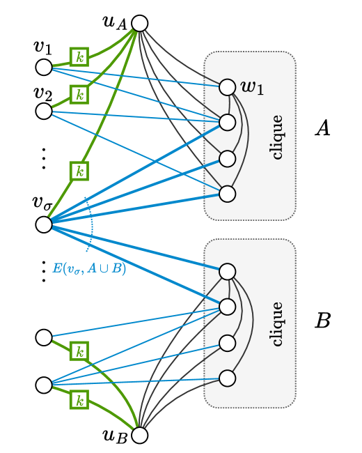
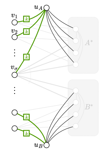
The set is further partitioned into vertex sets and , each of size at least . Every vertex has a unique identifier (ID), and we use any fixed arbitrary ID assignment from the set for all graphs in . Every graph is associated with a determining index . As we will see below, this name is motivated by the fact that the edges in the cut determine whether the graph is -connected.
Next, we define the edges of :
-
(E1)
and are cliques.
-
(E2)
For every , we add the edge , and, similarly, for every , we add .
We now define the edges in the cut : For every (), the incident edges are such that exactly one of the following two properties hold:
-
(E3)
and , or ; and there are parallel edges between and .
-
(E4)
and , and there are parallel edges between and .
We say that a node is -restricted if it satisfies (E3) and call -restricted if (E4) holds. Note that (E3) holds for a node even in the case that there are no edges at all between and .
Node , on the other hand, has exactly edges to nodes in , and
-
(E5)
there are parallel edges between and .
Moreover, one of the following two conditions hold:
-
(C0)
and ;
-
(C1)
and .
We point out that (E3), (E4), and (E5) require the input graph to be a multi-graph. This can be avoided by simply replacing and by cliques of size if desired, without changing the asymptotic bounds. Apart from the list of their neighbors, we provide additional power to the algorithm by revealing to each node whether it is -restricted, -restricted, or . Clearly, this can only strengthen the lower bound. Figure 1 shows an example of a graph .
We now state some properties of this construction. The next lemma is immediate from the description:
Lemma 1.
Every node is either , -restricted, or -restricted. Moreover, knows this information as part of its initial state.
Lemma 2.
Graph is -edge connected if and only if (C1) holds.
Proof.
Let be the subset of nodes that are -restricted, i.e., satisfy (E3), and also include in . Similarly, we define to contain all -restricted nodes, which satisfy (E4). Every has parallel edges to , which itself has an edge to each node in . Since is a clique of size at least , it follows that there are at least edge-disjoint paths between every pair of nodes in , which implies that is -edge connected. A similar argument shows that , , and induce a -edge connected subgraph. By properties (E1)-(E5), any edge in the cut must be in . Thus, the graph is -edge connected if and only if Case (C1) occurs. ∎
3 Existence of Indistinguishable Separated Pairs
As our overall goal is to prove Theorem 1, we assume towards a contradiction that each node sends at most bits throughout this section.
For a node , we call the subset of its neighbors in its -neighborhood. Here, our main focus will be to show that there is a way to choose the partition of that has properties suitable for our simulation in Section 5.
Definition 1 (Separated Pair).
We say that two -neighborhoods and form a separated pair for with respect to and , when the following are true:
-
•
if ’s -neighborhood corresponds to , then condition (C0) holds. In other words, and
-
•
if ’s -neighborhood is given by , then condition (C1) holds. Thus, and
Hence, if ’s -neighborhood is , the graph is -edge connected whereas if it is , then the graph is not -edge connected.
Since node has exactly neighbors in according to our lower bound graph description, we know that the set of all -neighborhoods of is of size . For technical reasons, however, we need to ensure that any pair of possible -neighborhoods of have an intersection that is at most a small constant fraction of . The proof of the next lemma follows via the probabilistic method and similar to Lemma 6 in [KNP+17a].444This is Lemma 7 in the full version of their paper on arXiv [KNP+17b]. We include a full proof in Appendix A for completeness.
Lemma 3.
Consider a set family , any small , and any positive integer . There exists a set family such that, for any two distinct , we have , and .
Instantiating Lemma 3 with and a suitable small constant , shows that
| (4) |
Given an arbitrary set , we say that is a partition of and each set is called a block of , if and all blocks are pairwise disjoint. For a fixed partition of and any , we define the projections and , and we also define the resulting image sets and . Consider the algorithm executed by some node . Let us assume that, for the time being, , and that node is equipped with ID . Together with the node IDs in its neighborhood, this fully determines the message sends to the referee. In particular, can send at most distinct messages, and hence the given algorithm induces a partition of into at most distinct blocks, where each block is a set of -neighborhoods for which sends the same message to Charlie. Let denote the largest one of these blocks, and observe that We emphasize that the depends on the ID of ; it may be the case that the resulting set contains a completely different set of neighborhoods for node (). Recall from Lemma 1 that a node may deduce whether by inspecting its degree and, consequently, the algorithm at may behave differently when compared to the case where is either -restricted or -restricted. That is, for a given partition of , the message sent by any -restricted node () induces a partition on , whereas the message sent by a -restricted node induces a partition on .
The next definition places some additional restrictions on a separated pair with respect to the three partitions , , and , which we will leverage in Section 5.
Definition 2 (Indistinguishable Separated Pair).
We say that and form an indistinguishable separated pair for , if the following properties hold:
-
(i)
and are in the same block of .
-
(ii)
and are distinct and in the same block of , and
-
(iii)
and are distinct and in the same block of .
-
(iv)
and form a separated pair for .
Lemma 4.
Suppose that we obtain the partition by assigning each vertex in uniformly at random to either or . Consider any . Then, with probability at least , there exist distinct that form an indistinguishable separated pair for .
Proof.
We start by defining additional partitions and that we obtain from and , respectively, as follows: For each block , we define
Partition has exactly the same number of blocks as , and we obtain from by defining it as the set containing all elements in . Analogously, we construct , which will have the same number of blocks as , and, for each , we get block , which contains all elements in . Thus, the number of blocks in , , and is at most , and all three of them partition the set given by Lemma 3.
To show the existence of the sought sets and , we need the following combinatorial statement:
Claim 1.
Let be a set of size , and let be partitions of , such that the number of blocks in each of the partitions is at most . Then, for every , there exists a block in that contains at least elements that are in the same block in each of the partitions .
Proof of Claim 1.
The case is immediate by the pigeonhole principle. For the inductive step, assume that the claim is true for some . That is, there is some block containing at least elements that are also in the same block in each of the partitions . Again, by the pigeonhole principle, we conclude that there exists a block that has at least elements of , as required. ∎
Instantiating Claim 1 with and partitions , , and , it follows that there exists a set , such that all sets in are in the same block in all three partitions. Moreover, (4) tells us that
Without loss of generality, assume that is even, and pair up the sets in in some arbitrary way. Let denote this set of pairs, and observe that
| (5) |
Consider any pair , and note that we have already shown that Property (i) of Definition 2 holds. To show Properties (ii) and (iii), suppose that . By construction of , we know that there exist some where is a block in , such that and , and, analogously, it follows that and are in a common block of .
To complete the proof, we need to bound the probability that and form a separated pair. Note that this will also imply and , by Definition 1 (see page 1).
Since , it must be true that either or . Without loss of generality, we can assume the former inequality holds—otherwise, simply exchange and . Recalling that , we know that , which means that, conditioned on , there are still at least
| (6) |
elements of , whose random assignment is not fixed by the conditioning. Let be the largest even integer such that and note that
| (7) |
Fix some order of the elements in , and define () to be the indicator random variable that is if and only if the -th element is in . Let . Our goal is to show that . In the worst case, all elements in lie in , and hence . Therefore, we need to make use of the following anti-concentration result to show that there is a sufficiently large probability for :
Lemma 5 (Proposition 7.3.2 in [MV01]).
Let be even, be independent random variables, where each takes the values of and with probability Let . For any integer , it holds that
To apply Lemma 5, define to be an integer such that
| (8) |
and note that holds, as long as since . By Lemma 5, we have
Recalling (5), it follows that the probability that none of the pairs in is a separated pair is at most
which is at most for sufficiently large .
It follows that one of the pairs in , all of which satisfy Properties (i)-(iii), is a separated pair with probability at least , which shows Property (iv) and completes the proof of Lemma 4. ∎
Recall that . For a randomly chosen partition of , Lemma 4 implies that a constant fraction of the nodes has indistinguishable separated pairs in expectation. Therefore, there must be some concrete choice for that ensures these properties. We are now ready to summarize the main result of this section while recalling the assumed upper bound on the message size:
4 The Problem
We now introduce a communication complexity problem in a 3-party model, whose hardness turns out to be crucial for obtaining a lower bound for deciding -edge connectivity in the sketching model.
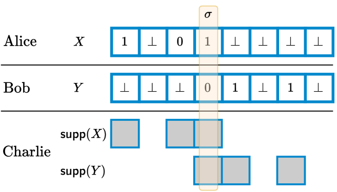
In the problem, we are given two positive integers and , where , and there are three players Alice, Bob, and Charlie. We focus on one-way communication protocols, where Alice and Bob each send a single message to Charlie, who outputs the result. Alice’s input is a ternary vector of length , denoted by , and, similarly, Bob gets a vector . We use to denote the support of a vector , i.e., the set of indices in , for which . Charlie does not know anything about and , except and .
Definition 3 (Valid Instance for ).
The tuple is a valid instance for , if and the following properties hold:
-
(P1)
There is exactly one index such that , where denotes the XOR operator.
-
(P2)
For every , it holds that or .
In conjunction, Properties (P1) and (P2) ensure that , and thus Charlie can deduce the value of directly from his input. To solve the problem, Alice and Bob each send a single message to Charlie, who must output “yes” if and , and “no” otherwise. See Figure 2 for an example.
4.1 Relationship to Other Problems in Communication Complexity.
In [AAD+23], the authors define the Leave-One Index problem (Problem 3 in [AAD+23]), where there are three players Alice, Bob, and Charlie. Alice and Bob hold the same string and Charlie knows an index . In addition, Alice has a set and Bob has a set with the property that , and the goal is that the players output , whereby the order of communication is Alice, Bob, and then Charlie. We point out that Leave-One Index lacks an important requirement of the problem, namely that Charlie also knows the exact support sets (not just their size) of the sets and given to Alice and Bob, which is crucial for the correctness of our simulation. Thus, it is unclear whether there exists a reduction between these problems.
The uniqueness of the shared index may give the impression, at first, that is related to a (promise) variant of computing the set intersection. However, we doubt the existence of a straightforward reduction, as, for the problem, the input vectors of Alice and Bob are ternary, and Charlie knows the (single) intersecting index as well as the support of the two input sets.
4.2 Hardness of the Problem
We now show that either Alice or Bob needs to send a message of size bits to Charlie in the worst case.
Theorem 2 (restated).
For any sufficiently large , there exists an such that the deterministic one-way communication complexity of in the simultaneous 3-party model is , where each -length input vector has support .
Proof.
Consider any protocol for and let be the worst case length of any message sent. Assume towards a contradiction that
| (9) |
Suppose that we fix Alice’s support to be a set of indices from , where is an integer parameter described below. We can partitions her possible input vectors into blocks such that the -th block contains all inputs on which Alice sends the number to Charlie. Clearly, the largest block in this partition contains at least inputs. Observe that there must exist a set of indices in such that, for each , there are inputs such that , i.e., Alice sends the same message for two inputs in which the bit at index is and , respectively. We say that index is flipped for , and we refer to as Alice’s flipped indices for support . Similarly, we can identify a set of flipped indices for Bob by partitioning all possible input vectors with support into blocks. Note that and need not be the same since Alice and Bob can execute different algorithms.
A crucial observation is that the algorithm fails, if there exist support sets and such that
-
(a)
, and
-
(b)
.
These conditions imply that the important index is flipped for Alice’s as well as Bob’s support. In more detail, this means that there are two inputs and for Alice that are in the same block , where and Alice sends the same message , and there are two inputs and in the same block , where , for which Bob sends , thus causing Charlie to fail in one of the (two) valid input combinations.
We show that if an algorithm manages to avoid (a) and (b) for all possible pairs of support sets, then it must send at least bits. Let be the set family of all possible -element support sets for the inputs of Alice and Bob. For each , define
which means that contains every support set where is a flipped index for of Alice, and we define analogously.
For the rest of the proof, if a statement holds for both and , we simply omit the superscript and write instead. Recall that each support contains at least flipped indices, i.e., and . This tells us that must be a member of at least of the set families, and thus
| (10) |
Consider and . The only way to avoid (a) and (b) is if and are not valid choices for the support of Alice’s input and Bob’s input , respectively (see Def. 3), which is the case if ; (recall that is impossible since ). For any , we can obtain a new set family by removing the index from each set in , i.e.,
The correctness of the assumed protocol implies the following:
Fact 1.
Set families and form a cross-intersecting family, which means that
| (11) |
Next, we employ an upper bound on the sum of the cardinalities of any two cross-intersecting set families:
Lemma 6 ([HM67]).
Let and be such that each is a family of -element sets on the same underlying set of size and assume that and are cross-intersecting. If , then
4.3 A Deterministic Algorithm for
The argument developed for our lower bound proof in Section 4.2 inspires the design of a simple deterministic algorithm that allows Alice and Bob to save a single bit by sending messages of length under certain conditions. As this is not needed for proving our main result, we relegate the details to Appendix B.
Theorem 3.
If , then there exists a deterministic one-way protocol for in the simultaneous -party model, such that Alice and Bob send at most bits to Charlie.
5 Simulation
In this section, we show how Alice, Bob, and Charlie can jointly simulate a given -edge connectivity algorithm in the 3-party model to solve the problem, for some given integers and , assuming that the sketches are sufficiently small for Corollary 1 to hold.
We now describe the details of the simulation and how the players can create the lower bound graph (see Sec. 2), given a valid instance of . First, each player locally computes
| (15) |
which will correspond to the number of nodes in the graph that the players construct. According to Corollary 1, there is a partitioning of into , as well as a set of size at least vertices, with the property that there exist indistinguishable separated pairs (see Def. 2), for each of the nodes in . We use to denote the first nodes in , ordered by IDs. Note that the players know, in advance, the IDs in the sets , , , , as these are fixed for all possible lower bound graphs in . Furthermore, they can also pre-compute the indistinguishable separated pair , for every , as these are fully determined by fixing , , and the algorithm at hand.
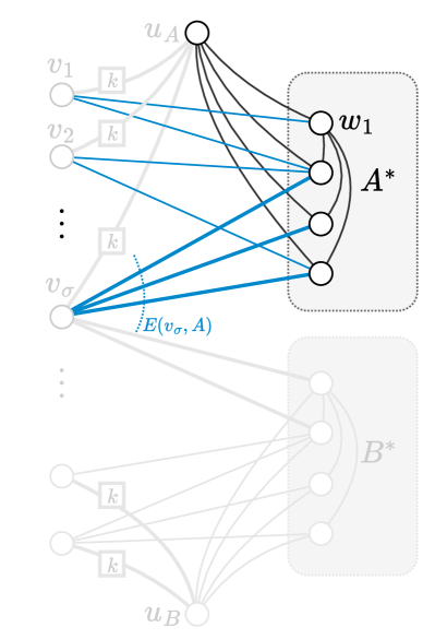
Alice’s and Bob’s Simulation:
Alice simulates all nodes in , whereas Bob is responsible for the nodes in . See Figures 3(a) and 3(b) for an example. First, Alice creates a clique on and connects to each node in this clique. Then, for each where , Alice inspects the input and adds edges incident to the nodes in as follows:
-
•
If , then she includes the edges between and the nodes in .
-
•
On the other hand, if , then Alice adds all edges connecting to .
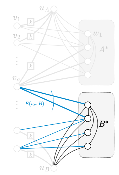
Bob adds a clique on and, analogously to Alice, includes an edge between and each node in . Next, we describe how Bob creates the edges between and node , for each :
-
•
If , then he adds edges between and .
-
•
If , he connects to each node in .
Finally, Alice and Bob locally execute algorithm to compute the sketches produced by their simulated nodes in and , respectively, which they send to Charlie.
Charlie’s Simulation:
Charlie is responsible for computing the sketches for , , and all nodes in , and he will also simulate the referee. To this end, he creates edges between and each node in —recall that these edges were also created by Alice for simulating the nodes in —and he also connects to every via parallel edges. Note that contains every such that or , whereby the latter case is equivalent to . Charlie also includes parallel edges connecting to every where . Similarly, he adds edges between and each node in . See Figure 3(c).
Next, we describe how Charlie simulates the nodes in :
-
•
First, consider the crucial node , where : Since Charlie does not know whether Alice and Bob used or for creating the edges between their nodes in and , he cannot hope to faithfully recreate the entire neighborhood of . However, what he can do instead is to directly compute the sketch that algorithm produces for node , in the case that . To see why this is true, recall that or form an indistinguishable separated pair, and Charlie knows the block in partition that contains as well as . This ensures that sends the same sketch given either neighborhood.
-
•
For any node (), Charlie proceeds analogously as in the case , with the only difference being that he no longer uses for identifying the common block that contains and (and deriving ’s sketch). Instead, if is -restricted (i.e., ), then he uses to find the common block that contains and and uses the associated block in (see Page 4) to derive ’s sketch. Otherwise, must be -restricted (), prompting him to find the common block in , and compute ’s sketch accordingly.
-
•
Charlie can directly simulate the remaining nodes in , i.e., every
since the only edges added for are parallel edges to .
Charlie simulates that the referee receives the sketches sent by the nodes in , , and , as well as the messages that it received from Alice and Bob for the nodes in and , which is sufficient for invoking and obtaining the decision by the referee. Charlie answers “yes” if and only if the decision was that the graph was -edge connected.
5.1 Correctness and Complexity Bounds of the Simulation
As made evident by the above description, our simulation constructs only certain graphs in . In particular, these are graphs where all edges in the cut are determined by separating pairs. We start by formalizing this restriction:
Definition 4.
Consider any graph and recall the existence of set , the partition , and the separating pairs for each , guaranteed by applying Corollary 1 to algorithm . We say that is compatible with a valid instance of if and, for every :
-
1.
If , then .
-
2.
If , then .
-
3.
If , then .
-
4.
If , then .
-
5.
If or , then has edges to .
-
6.
If , then has edges to .
Lemma 7.
Let be a graph that is compatible with an instance of . It holds that is -edge connected if and only if the solution to is “yes”, i.e., and .
Proof.
Since is a compatible graph, we know that . Thus, it follows from Lemma 2 that is -edge connected if and only condition (C1) holds, i.e., and . Since form a separated pair, we know from Definition 1 that this is satisfied for . According to Definition 4, we use to determine the neighbors of in if and only if and , which proves the correspondence between -edge connectivity and the solution to . ∎
Equipped with Definition 4, we are ready to show that the sketches produced by the simulation indeed correspond to an actual execution of on a suitable graph in .
Lemma 8.
Suppose that algorithm has a maximum sketch length of bits. Then, Charlie provides as input to the referee in the simulation the same set of sketches that the referee receives when executing algorithm on a graph compatible with the instance .
Proof.
Since the players construct a graph , where , it follows from (2) (on page 2) that . According to Corollary 1, this implies that the set must have a size of for some constant , which ensures that the set of size exists. Recall that all players can compute , since this is fully determined by the algorithm at hand (i.e., ) and the parameters , , and . We now argue that the simulation computes the correct sketch for every type of node in graph :
-
•
Nodes and : These nodes are only simulated by Charlie who knows , , and thus also . By the description of the simulation, Charlie creates their incident edges in a way that satisfies Points 5 and 6 of Definition 4.
-
•
Node : Without loss of generality, assume that ; the case is symmetric. In the execution on the compatible graph , the edges in the cut are fully determined by the separating pairs , which corresponds to how Alice creates the edges incident to in the simulation. Moreover, Alice will also add an edge , which ensures the same sketch for as in the actual execution.
-
•
Node : According to the simulation, Charlie will select one of the blocks , where , and , with the property that each of the blocks contains . Recall that these blocks exist due to Corollary 1. Let be the associated block of , and be the associated block of , see Page 4. If , then he computes where corresponds to the message sent by for the inputs in ; otherwise, if , then he computes . Finally, in the case that , he computes instead. A crucial observation is that, even though Charlie does not know whether Alice used or to create the edges in , this does not prevent him from computing the correct sketch for , since and are guaranteed to be in the same block in each of the partitions; a similar argument applies to the edges in .
-
•
Node : These nodes do not have any edges to . Instead, Charlie only creates parallel edges to , which matches the neighborhood of in the compatible graph . ∎
Lemma 9.
Suppose there exists a deterministic -edge connectivity algorithm, with the property that every node sends a sketch of length at most bits, when executing on . Then, has a deterministic communication complexity of bits.
Proof.
By Lemma 8, Charlie invokes the referee with the same set of sketches as in the execution of algorithm on the compatible graph . Thus, correctness follows directly from Lemma 7.
Next, we show the claimed bound on the communication complexity of . By (15) (see page 15), we know that the size of is chosen such that . Since every node in sends a sketch of at most bits in the simulation, and these are all the nodes simulated by Alice and Bob, sending these concatenated sketches to Charlie requires at most
| (16) |
bits, where we have used (3) in the second-last equality. ∎
6 Combining the Pieces
We now use the results from the previous sections to prove Theorem 1.
Theorem 1 (restated).
Every deterministic algorithm that decides -edge connectivity on -node graphs in the distributed sketching model has a worst case message length of bits, for any super-constant , where is a suitable constant.
Let be the maximum length of a sketch. Suppose that every node in sends at most bits, and consider an instance of . Lemma 9 tells us that we can solve an instance of if Alice and Bob send a message of bits. Since , the messages sent is thus bits. We obtain a contradiction to Theorem 2 which states that any deterministic algorithm for must send bits in the worst case.
7 Conclusion and Open Problems
A problem left open by our work is the complexity of randomized sketching algorithms for deciding -edge connectivity. As outlined in Section 1, the existing lower bound approach for graph connectivity does not appear to be amenable to a straightforward generalization. This suggests that either new technical ideas are needed for proving such a bound, or perhaps there is indeed a more efficient randomized algorithm:
Open Problem 1.
What is the sketch length of deciding -edge connectivity, if we allow a small probability of error?
Our result implies that any deterministic sketching algorithm must send sketches of near-linear (in ) bits in the worst case. While the AGM sketches [AGM12a] yield an upper bound of bits, currently there is no non-trivial deterministic upper bound:
Open Problem 2.
Is there a deterministic -edge connectivity algorithm that matches the best known randomized upper bound of bits on the sketch length?
Finally, we point out that our techniques do not shed light on the most fundamental open problem in this setting, namely (1-edge) connectivity:
Open Problem 3.
Can we solve connectivity deterministically in the distributed sketching model if messages are of length ?
Acknowledgements
The authors would like to thank the anonymous reviewer for pointing out the relationship between the problem and the Leave-One Index problem of [AAD+23].
Appendix
Appendix A Proof of Lemma 3
Lemma 3 (restated).
Consider a set family , any small , and any positive integer . There exists a set family such that, for any two distinct , we have , and .
Proof.
The proof is similar to Lemma 6 in [KNP+17a]. Fix . We choose independently and uniformly at random from . We first bound the expected size of the overlap of two given subsets. Consider two distinct indices , and define indicator random variables such that if and only if the -th element of intersects with , which happens with probability , and thus . While the variables are not independent, they are negatively dependent, and thus we can use a Chernoff bound to show concentration. For , we get
It follows by a union bound over the possible pairs of subsets that a set family with the required bounded intersection property exists with nonzero probability. Note that
| (since ) | |||
∎
Appendix B Proof of Theorem 3
Theorem 3 (restated).
If , then there exists a deterministic one-way protocol for in the simultaneous -party model, such that Alice and Bob send at most bits to Charlie.
Proof.
Consider an input vector with where . We can obtain a binary string of length from by simply removing all from the vector. In other words, the binary string of is . For the rest of the proof, we use to refer to the input vector or its binary string representation depending on the context.
We define to be the mapping of the bit string of to a -length bit string that we get by removing . That is,
Our algorithm determines the message sent by a party given the input vector to be , whereby is chosen in a way that guarantees that Charlie can compute the output correctly. Note that, given and , the only bit values of that Charlie can not deduce with certainty is the value at index , i.e., . Now, consider a valid input pair and , where . Upon receiving the messages and sent by Alice and Bob respectively, for some values and , Charlie can deduce and only if at least one of or is not .
In the following, we describe a protocol on how to choose the value so that Charlie can compute correctly: We construct a partition of into blocks such that for each :
-
(a)
For all , we have .
-
(b)
For all in , it holds that .555The reader may notice that the set families are defined analogously as in the lower bound proof in Section 4.2.
To see why Properties (a) and (b) are sufficient, consider and such that . Let and are such that and . The message sent by Alice and Bob given input and is thus and , respectively. By the properties of the partition, it follows that . Hence, at least one of them is not equal to , which allow Charlie to deduce the correct value of and .
To complete the proof, we give a concrete construction of the blocks : We partition into intervals, each of length , except possibly one interval, where the length is either or . We define to be the successor of in the interval containing , following the cyclic order. For instance, if the interval is , then
for Since we are considering cyclic order, the intervals are referred to as cycles. Note that if a cycle has only one element, say , we set to be an arbitrary element different from .
Let . We define to be the set that contains all in such that both and are in , i.e., . To ensure and are disjoint, we remove any that occurs in from one of them. It is straightforward to verify that the resulting indeed satisfy Properties (a) and (b).
It remains to show that . Consider . Recall that there are elements in and cycles. Given that from the assumption, there must exists distinct elements and in such that they are in the same cycle. Hence is in some . ∎
References
- [AAD+23] Vikrant Ashvinkumar, Sepehr Assadi, Chengyuan Deng, Jie Gao, and Chen Wang. Evaluating stability in massive social networks: Efficient streaming algorithms for structural balance. In APPROX/RANDOM, 2023.
- [AGM12a] Kook Jin Ahn, Sudipto Guha, and Andrew McGregor. Analyzing graph structure via linear measurements. In Proceedings of the twenty-third annual ACM-SIAM symposium on Discrete Algorithms, pages 459–467. SIAM, 2012.
- [AGM12b] Kook Jin Ahn, Sudipto Guha, and Andrew McGregor. Graph sketches: sparsification, spanners, and subgraphs. In Proceedings of the 31st ACM SIGMOD-SIGACT-SIGAI symposium on Principles of Database Systems, pages 5–14, 2012.
- [AKO20] Sepehr Assadi, Gillat Kol, and Rotem Oshman. Lower bounds for distributed sketching of maximal matchings and maximal independent sets. In PODC ’20: ACM Symposium on Principles of Distributed Computing, Virtual Event, Italy, August 3-7, 2020, pages 79–88, 2020.
- [BMN+11] Florent Becker, Martin Matamala, Nicolas Nisse, Ivan Rapaport, Karol Suchan, and Ioan Todinca. Adding a referee to an interconnection network: What can (not) be computed in one round. In 2011 IEEE International Parallel & Distributed Processing Symposium, pages 508–514. IEEE, 2011.
- [BMRT14] Florent Becker, Pedro Montealegre, Ivan Rapaport, and Ioan Todinca. The simultaneous number-in-hand communication model for networks: Private coins, public coins and determinism. In Structural Information and Communication Complexity - 21st International Colloquium, SIROCCO 2014, Takayama, Japan, July 23-25, 2014. Proceedings, pages 83–95, 2014.
- [GMT15] Sudipto Guha, Andrew McGregor, and David Tench. Vertex and hyperedge connectivity in dynamic graph streams. In Proceedings of the 34th ACM SIGMOD-SIGACT-SIGAI Symposium on Principles of Database Systems, pages 241–247, 2015.
- [HKT+19] Jacob Holm, Valerie King, Mikkel Thorup, Or Zamir, and Uri Zwick. Random k-out subgraph leaves only o(n/k) inter-component edges. In 60th IEEE Annual Symposium on Foundations of Computer Science, FOCS 2019, Baltimore, Maryland, USA, November 9-12, 2019, pages 896–909, 2019.
- [HM67] Anthony JW Hilton and Eric C Milner. Some intersection theorems for systems of finite sets. The Quarterly Journal of Mathematics, 18(1):369–384, 1967.
- [JLN18] Tomasz Jurdzinski, Krzysztof Lorys, and Krzysztof Nowicki. Communication complexity in vertex partition whiteboard model. In International Colloquium on Structural Information and Communication Complexity, pages 264–279. Springer, 2018.
- [JN17] Tomasz Jurdzinski and Krzysztof Nowicki. Brief announcement: on connectivity in the broadcast congested clique. In 31st International Symposium on Distributed Computing (DISC 2017). Schloss Dagstuhl-Leibniz-Zentrum fuer Informatik, 2017.
- [Juk01] Stasys Jukna. Extremal combinatorics: with applications in computer science, volume 29. Springer, 2001.
- [KN97] Eyal Kushilevitz and Noam Nisan. Communication Complexity. Cambridge University Press, 1997.
- [KNP+17a] Michael Kapralov, Jelani Nelson, Jakub Pachocki, Zhengyu Wang, David P Woodruff, and Mobin Yahyazadeh. Optimal lower bounds for universal relation, and for samplers and finding duplicates in streams. In 2017 IEEE 58th Annual Symposium on Foundations of Computer Science (FOCS), pages 475–486. Ieee, 2017.
- [KNP+17b] Michael Kapralov, Jelani Nelson, Jakub Pachocki, Zhengyu Wang, David P Woodruff, and Mobin Yahyazadeh. Optimal lower bounds for universal relation, and for samplers and finding duplicates in streams. arXiv preprint arXiv:1704.00633, 2017.
- [KRW95] Mauricio Karchmer, Ran Raz, and Avi Wigderson. Super-logarithmic depth lower bounds via the direct sum in communication complexity. Computational Complexity, 5:191–204, 1995.
- [McG14] Andrew McGregor. Graph stream algorithms: a survey. ACM SIGMOD Record, 43(1):9–20, 2014.
- [MT16] Pedro Montealegre and Ioan Todinca. Brief announcement: deterministic graph connectivity in the broadcast congested clique. In Proceedings of the 2016 ACM Symposium on Principles of Distributed Computing, pages 245–247, 2016.
- [MV01] Jiří Matoušek and Jan Vondrák. The probabilistic method. Lecture Notes, Department of Applied Mathematics, Charles University, Prague, 2001.
- [NY19] Jelani Nelson and Huacheng Yu. Optimal lower bounds for distributed and streaming spanning forest computation. In Proceedings of the Thirtieth Annual ACM-SIAM Symposium on Discrete Algorithms, SODA 2019, San Diego, California, USA, January 6-9, 2019, pages 1844–1860, 2019.
- [Pin64] Mark S Pinsker. Information and information stability of random variables and processes. Holden-Day, 1964.
- [PP20] Shreyas Pai and Sriram V Pemmaraju. Connectivity lower bounds in broadcast congested clique. In 40th IARCS Annual Conference on Foundations of Software Technology and Theoretical Computer Science (FSTTCS 2020). Schloss Dagstuhl-Leibniz-Zentrum für Informatik, 2020.
- [Rob23] Peter Robinson. Distributed sketching lower bounds for k-edge connected spanning subgraphs, BFS trees, and LCL problems. In 37th International Symposium on Distributed Computing (DISC 2023), pages 32–1. Schloss Dagstuhl–Leibniz-Zentrum für Informatik, 2023.
- [Yu21] Huacheng Yu. Tight distributed sketching lower bound for connectivity. In Proceedings of the 2021 ACM-SIAM Symposium on Discrete Algorithms, SODA 2021, Virtual Conference, January 10 - 13, 2021, pages 1856–1873, 2021.