Developing an Agent-Based Mathematical Model for Simulating Post-Irradiation Cellular Response: A Crucial Component of a Digital Twin Framework for Personalized Radiation Treatment
Abstract
In this study, we present the Physical-Bio Translator, an agent-based simulation model designed to simulate cellular responses following irradiation. This simulation framework is based on a novel cell-state transition model that accurately reflects the characteristics of irradiated cells. To validate the Physical-Bio Translator, we performed simulations of cell phase evolution, cell phenotype evolution, and cell survival. The results indicate that the Physical-Bio Translator effectively replicates experimental cell irradiation outcomes, suggesting that digital cell irradiation experiments can be conducted via computer simulation, offering a more sophisticated model for radiation biology. This work lays the foundation for developing a robust and versatile digital twin at multicellular or tissue scales, aiming to comprehensively study and predict patient responses to radiation therapy.
Keywords: Cell State Transition Theory, Radiation-induced Cellular Effects, Radiation-induced Bystander Effect, Cell State Model, Cell Cycle Arrest, Digital Twin
1 Introduction
“Digital twins” are software replicas that simulate the dynamic functions and potential failures of engineered products and processes. In the context of radiation oncology, patient-specific digital twins can integrate known human physiology and immunology with real-time, patient-specific clinical data to produce predictive computer simulations of tumor response following radiation treatment. These medical digital twins represent a powerful addition to the arsenal of tools used to combat cancer, enabling the development of optimized, personalized treatment protocols. By combining mechanistic knowledge, observational data, and patient medical histories with advanced experimental techniques, mathematical and computational modeling, and the power of artificial intelligence (AI), digital twins can significantly enhance our ability to quantitatively characterize and treat cancer. A robust digital twin modeling framework should incorporate models at subcellular, multicellular, and tissue scales to study and predict patient responses to radiation therapy comprehensively. This multiscale approach ensures a detailed and accurate representation of the biological processes involved, ultimately leading to more effective and individualized radiation treatment strategies.
One crucial component of this digital twin framework is a mathematical model that simulates radiation-induced cellular effects at the cellular scale. These effects can be viewed as the results of physical interactions within the cell, as all subsequent complex biological reactions stem from the initial energy deposition process. It is noteworthy that after radiation deposits energy in a cell, a very complex and continuous biological process ensues. Given the current state of simulation techniques, it is impractical to follow every detailed biochemical process to study radiation effects. Therefore, it is more effective to consider the complex biological processes from a mechanistic system perspective, using the results of physical interactions between radiation and the cell as inputs to the cell response system, and the final possible phenotypes of the cell as outputs.
Historically, mechanistic models have been employed to simulate post-irradiation cellular responses, with numerous models proposed [1, 2, 3, 4, 5]. These models have played a significant role in the fields of radiation biology and radiation therapy. However, several challenges remain. For instance, new phenomena such as non-targeted effects have been recognized in the radiation biology community, but most conventional modeling frameworks adhere strictly to target theory related models. A generalized mechanistic model that simulates both target and non-target effects is still missing. Additionally, most models heavily rely on assumptions that treat unknown mechanisms as a black box, lacking a detailed correlation between the radiation dose and its microscopic outcomes at both the cell and tissue levels.
In response to these challenges, several improvement strategies should be considered for model design and implementation. We propose that a better model should have the following characteristics:
-
•
The model incorporates a literature-based, rigorous mathematical formula that generalizes both target and non-target effects into a single mechanistic model, and it should quantitatively recapitulate measured data.
-
•
Following the principle of parsimony, the model includes only the most critical components based on literature, which can explain the radiation effect.
-
•
The model, parameterized to measured data, provides conceptual insights into radiation effects.
-
•
The model is "as mechanistic as possible" and should use parameters with clear biophysical meaning.
-
•
In addition to considering extensive observations of factual and empirical knowledge, the model incorporates quantification principles familiar in physical sciences to provide a different perspective on quantifying radiation effects.
-
•
The model is parameterized using population data, representing a hypothetical non-existent average cell, allowing the model to capture generalized effects and be reused in different applications.
-
•
The new mechanistic model could be designed and implemented in a modularized way, integrating physical, chemical, and biological phases into the simulation framework.
In this study we propose a novel agent-based mathematical model that simulates the post-irradiation cellular response. From a metaphorical perspective, the mechanistic model for interpreting the radiation response after irradiation functions as a “translator” between physical interactions and biological interactions. So, we name our model as Physical-Bio Translator. In the current development of the Physical-Bio Translator, several major functions have been implemented, including simulating the bystander effect on cells, and predicting the possible phenotypes after irradiation. In this paper, we will present Physical-Bio Translator in detail.
2 Methods and Materials
In this section, we introduce all the components of our developed agent-based mathematical model for simulating the radiation-induced cellular response.
2.1 Cell-State Model
Following standard approaches, our cell-state model quantifies the possible cell phenotypes transition in temporal after irradiation [6, 7, 8].
2.1.1 Cell State Classification
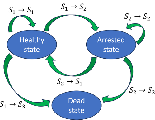
We define three major cell states: Healthy, Arrested, and Dead. A Healthy cell maintains its basic proliferation potential with no or very light damage. An Arrested cell has its cycle halted in a specific cell-cycle phase. A Dead cell has suffered irreparable damage and suspends material exchange with the extracellular matrix (ECM). We assume that the dead state is an average phenomenon of all the possible cell death routes, such as apoptosis, necrosis, etc. Each of these cell states differs depending on the cell’s phase in the cell cycle: G1, S, G2, or M.
2.1.2 Cell State Transitions
The allowed state transitions are:
-
•
From Healthy to Arrested or Dead.
-
•
From Arrested to Dead or Healthy.
Dead cells stay dead. Transitions depend only on a cell’s current state. These state transition rules are based on radiation biology experiments. For instance, 1) A high dose causing direct cell death corresponds to the state transition from Healthy to Dead; 2) A moderate dose causing cell-cycle arrest corresponds to the state transition from Healthy to Arrested; 3) Cell apoptosis after failed cell damage repair during cell-cycle arrest, corresponds to the state transition from Arrested to Dead; 4) A dead cell does not have capacity to repair damage, so theDead state is persistent. Because the dead state is an average phenomenon of different types of death, this formalism could be extended to include other definitions of cellular death types, e.g., cell apoptosis and necrosis. To model cell state transitions after radiation exposure, we propose state energy to quantify the radiation-induced damage to each cell. The state energy includes two parts: the direct state energy , which quantifies direct radiation-induced damage:
| (1) |
where is a constant and is the number of double-strand DNA breaks (DSBs) produced by direct radiation hitting the cell. The DSB is the most lethal DNA damage type to the cell, and here we aggregate all direct damage into an effective DSB number.
The indirect state energy quantifies the net damage from bystander signaling. The bystander signals emitted by a signaling cell can migrate and interact with other cells. In this work, we assume that the diffusion-reaction is the major process that contributes to the cell communication by bystander signals, and the receptor-ligand kinetics was considered to model the bystander signal and cell reaction process [9]. We describe the interaction by a second-order reaction depending on the bystander signal concentration and cell receptor concentration:
| (2) |
where is a constant, is the time after cell irradiation, is reaction rate coefficient at time , is the transient concentration of cell receptor concentration at time , and is the transient bystander signal concentration at .
Equation (2) integrates the absorption of bystander signals by the cell. For simplicity of denotation, we denote the integral of reaction rate as , i.e.
| (3) |
To be parallel to equation (1), we can write the indirect state energy as:
| (4) |
where is the bystander signal concentration absorbed in the cell. Both targeted and non-targeted cellular effect can lead to different level of DNA damage [10]. In this work, we propose that state energy is a measure of DNA damage induced by radiation including target effect and the bystander effect. State energy is dimensionless, and two types of state energy could be added together, then the total state energy of a cell could be as:
| (5) |
When a cell experiences a radiation dose directly or absorbs bystander signals, its state energy increases. When DNA damage is repaired, the state energy decreases. When state energy increases, a cell will have more potential to jump to higher energy cell states. We introduce another term, external perturbation energy, , to quantify the increase of the state energy. To quantify the energy state transition based on the transition rules, we introduce several basic propositions:
-
•
At a specific time, a cell can and only can stay in one specific energy state, and for each energy state, there is a corresponding state energy distribution. The details of the distribution will be explained below.
-
•
The cell state energy distribution will change if external perturbation energy is nonzero, and correspondingly, a cell will have certain probability of jumping to higher energy states if its state energy increases. A cell will have a certain probability of jumping to lower energy states if its state energy decreases, which corresponds to the cell damage reparation.
-
•
If a cell stays at the highest energy state (i.e. death state), there will be no further state transition. Also, if a cell stays at the lowest energy state (i.e. health state), its state energy cannot decrease.
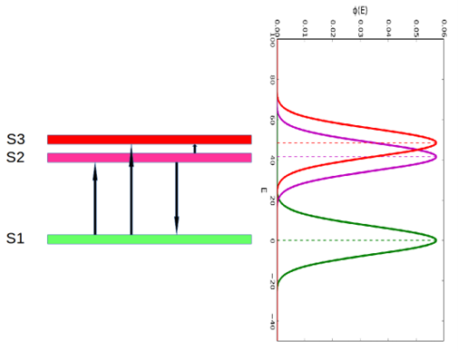
For a given level of dose to cells, some cells of a given type that are apparently identical will stay healthy, some will have cell cycle arrest and still others will die. In order to quantify the distribution of cell states, we introduce a distribution of cell state energies for each cell state. In this study, we have three cell states: , , and , representing the healthy state, arrested state and death state, respectively. Here we propose that for each cell state its state energy E follows a normal distribution . The state energy distribution of state could be written as:
| (6) |
where is the mean state energy of state , and is the standard deviation of state energy of state . It is noteworthy that could be taken as the most feasible state energy for state , and is a measure of the fluctuation of state energy distribution. One example of a state energy distribution is shown in Figure1. The biological implication of state energy distribution is that we often cannot determine a definite damage level for a certain cell phenotype after irradiation. Taking radiation-induced cell death for example, when we determine the lethal dose which induces cell death, we often observe that the lethal dose is within a dose interval instead of a single lethal dose. The same amount of radiation or bystander signal can cause stochastically different amounts of damage to identical cells.
When radiation-induced DNA damage is incurred, the cell state energy will increase, which will induce a change in the cell state energy distribution correspondingly. We assume that the shape of the state energy distribution will not change, but the mean state energy will shift. For instance, suppose the current energy state of the cell is , then if cell absorbs perturbation energy , its state energy distribution will be as:
| (7) |
After defining the state energy distribution, it is plausible to quantify the probability of state transitions. The cell state transition probability is quantified by calculating the overlapping integral of the state energy distribution.
The overlapping integral of two state energy distributions is written as:
| (8) |
where and are the state energy distribution functions of two cell energy states.
The computation of the overlapping integral for two state energy distributions, , depends on whether the two variances are equal or not. Here we start with the simpler case where we have . We then have
| (9) |
where is the cumulative distribution function of the normal distribution and it is as
It is obvious that , and if and only if those two normal distributions are identical. We use the overlapping integral as a measure of cell state transition probability between two states, and the transition probability from state to is:
| (10) |
Suppose initially at time , a cell stays at state . If it absorbs an external perturbation energy and its state energy distribution will shift to a possible higher energy state , then the transition probability from to is:
| (11) |
Based on equation (11), we can calculate the probabilities for all the possible transition routes. The possible cell state transition route is shown in Figure 2. The final transition route is selected based on a rejection algorithm based on Monte Carlo sampling [11]. The selection process is as follows:
-
•
if , where , the cell remains in
-
•
if , the cell transitions into
-
•
Otherwise, cell transitions into
2.1.3 Radiation Sensitivity in Different Cell Phases
Cells are known to have different radiation sensitivity in different cell phases. Cells in the G2 and M phases usually have higher radiation sensitivity, lower radiation sensitivity in the G1 phase, and the lowest radiation sensitivity during the latter part of the S phase. We define a radiation sensitivity factor for each cell phase. Here, we introduce a method to calculate the radiation sensitivity factor using the cell state transition rule we just introduced above.
For nomenclature simplicity, each cell phase is assigned an index i corresponding to the four cell phases where and corresponds to G1, corresponds to S, corresponds to G2, and corresponds to M. We denote as the mean state energy of state at cell phase, i.e., where and .
For cell phase G1, the transition probability from to after cell absorbs external perturbation energy is
| (12) |
Now we consider a less radiosensitive cell phase, S, the transition probability from to after absorbs energy is
| (13) |
From equation (12) and equation (13) we can know that transition probability is a function of . Here, we calculate the derivatives of equation (12) and equation (13) with respect to . We can have
| (14) |
where which is the normal distribution density function. Similarly, we can get
| (15) |
We define a radiation sensitivity factor f for each cell phase. We take for G1 phase, and the radiation sensitivity factors in other cell phases could be normalized according to . We propose that the radiation sensitivity factor for the cell phase G2 as:
| (16) |
Then we can have
| (18) |
Equation (18) shows the relationship between radiation sensitivity factor and the mean state energies.
2.1.4 Cell Arrest Duration Quantification
It is known that the cell cycle could be temporarily or permanently arrested for a while after cell irradiation. Here, we propose a method to calculate the cell arrest duration based on the cell state transition model. As well-studied experimentally [12, 13], the kinetics of DSB rejoining exhibits a fast initial rate, which then decreases with repair time. The most widely accepted description of this kinetic behavior uses two first-order components (fast and slow). This general two-repair-components model is used widely [14, 15, 16]. The main common characteristic of the model is assuming the fast repair and slow repair follow a first-order exponential decay scheme. Then the total DSB number after irradiation could be described as:
| (19) |
where is the DSB number in cell at time , and correspond to the weights of the two repair components respectively, and corresponds to the decay constants of repair components respectively. And we have .
We introduce two definitions for mathematical formalization. The transient arrest state is the state which will be released after a certain amount of time. The transient arrest duration is the total time for a cell staying at transient arrest state.
The cell state energy proposed in our model is a measure of DNA damage level. In this study, we propose that state energy also follows the same kinetics as radiation-induced DSB. The state energy with respect to time could be expressed as:
| (20) |
When a cell jumps to from , the state energy of will decrease with time because of the DNA damage repair. The probability of cell state transition from to at time will be as:
| (21) |
According to equation (20), we can know that
| (22) |
where is the initial cell state energy at . We take , so equation (21) could be written as:
| (23) |
Then we can know the jumping probability rate is as:
| (24) |
Based on equation (24), we can obtain the mean life time of which is the mean duration of transient arrest state. The mean lifetime of could be obtained by
| (25) |
Substituting back into equation (23) then the integration in equation (25) could be changed to as:
| (26) |
We can approximate equation (26) with the expansion of the term neglecting the higher order terms in the integration and we get the mean lifetime of that could be calculated as:
| (27) |
We see that the cell arrest duration could be determined by DNA repair kinetics and state energy distribution. From equation (27) we can know that the slow repair phase of DSB, which has the smaller half-life will dominate the transition duration. This is in line with one speculative view published in [17] that the slow homologous recombination repair (HRR) of DSB determines the length of cell arrest duration. Transient arrest duration is a measure of the time needed for cell state recovery.
2.2 Agent-based simulation
In this study, we use an agent-based simulation method to implement the cell-state model for simulating the cellular response after irradiation. By using a simplification of an agent-based approach that treats cells as simple interacting agents, we can simulate the interactions of tens of thousands to millions of cells, and we can describe the normally unreachable smaller-scale structure of tissues and organs. The agent model consists of two components, namely, cellular space and transition rule. Each cell is considered as a finite-state machine [18], and each cell has an identical pattern of local connections to other cells for input and output, along with boundary conditions if the lattice is finite. Each cell is denoted by an index and its state at time step is denoted as . The neighborhood of state of cell is denoted as . Cell updates its state according to the current state and the states of its neighbors.
| (28) |
At each time step, all cells update their state synchronously according to .
2.2.1 Simulating Cell Phase Transition
As soon as the duration of a given cell phase has passed, the transition to the next phase of the cell cycle occurs. The time at which the transition takes place varies in a random manner according to a distribution of durations of the cell cycle phases. A probability density function can be assigned to each phase such that the probability of the duration time for the phase having a value in the interval around t is given by . In this work, is defined as a Gaussian distribution [19]. In each phase, the phase duration time, , and a variance , which are identified with the mean and variance of . The probability density function of duration time is a half Gaussian distribution, and it is written as:
| (29) |
Naturally, without any perturbation, a cell will go through the normal cell cycle, and we can simulate the cell cycle progression based on the probability density distribution in equation [29]. We can use Monte Carlo sampling to determine the duration of one cell phase. For phase Gi, we can sample a duration length for it as
| (30) |
where and are random numbers.
We can determine the transition rule determined by time evolution as:
| (31) |
where is used to describe the cell phase transition result.
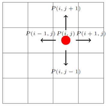
Cell cycle progression is dependent on external conditions, specifically the local nutrient availability (such as glucose concentration in the medium) and interaction with neighboring cells (integral pressure) [20]. In this work, we assume that all the cells are in good nutrient condition. The interaction with neighboring cells is considered by checking the contact inhibition condition of the cell. The cell will stay at quiescent state if there is no space for the daughter cells [21]. Regarding where to position the two daughter cells, one of the common rules is to position them randomly at the adjacent vacant sites. Taking an example as shown in Figure 3, if the grid lattice is filled by a cell, then we define a variable , otherwise . Then we can determine whether there is space for new cells in the system by checking the value of .
| (32) |
and apparently .
The transition rule determined by neighbor condition is as:
| (33) |
Then we can write the transition rule for cell phase transition as:
| (34) |
It is worth noting that the transition rule could be easily extended by incorporating other conditions which determine the cell phase transition process.
In this study, we used the cell phase ratio to describe the cell phase distribution, and the cell phase ratio of phase is defined as:
| (35) |
where is the cell phase ratio of cell phase, is the number of cells staying at phase and is the total number of cells.
2.2.2 Simulating Cell State Transition
The cell state transition is a continuous stochastic process evolving with time after cell irradiation. The cell state transition probability obtained by equation (11) is the total probability during the time until actual cell state transition (phenotype) is observed. In the agent-based model, the time is discretized into time steps and the probability of cell state transition should be determined for each time step. So here we introduce a model to quantify the probability of cell state transition in each time step. Firstly, the external perturbation energy for each cell is determined, then the probability of corresponding cell state transition is calculated based on in the time step. Secondly, the cell state transition decision is made based on the calculated transition probability.
The cell state transition is dependent on sources which contribute to . For instance, DSBs and bystander signals all can induce . The direct DSB is a more effective lethal damage compared to bystander signals, so it can induce the fast cell state transition. Relatively, the bystander signal is a less damaging agent which is subject to relatively constant and cyclic stresses to cells since the bystander signal will perpetuate in the cell culture until it decays away. In this work, considering the difference between those two external perturbation factors, we propose two types of cell state transition modes, i.e., delayed transition and instantaneous transition.
The instantaneous transition happens immediately after the cell absorbs external perturbation energy. The delayed transition is a relatively slow transition that happens after a certain time from the time when the cell absorbs external perturbation energy. For the delayed transition, the time-to-transition, , varies. In this work, we introduce a model to quantify the state transition as a failure process. First, we introduce a term, observation time , within which the radiation-induced cellular phenotype could be observed. The exact time of state transition is not known, and we can assume the time-to-transition as a random variable, , and it has a density function , then we can have
| (36) |
where is the cell state transition distribution function. The density function can be described in terms of as:
| (37) |
This can be interpreted as the probability that the cell state transition time will occur between the time and the next time .
Within the observation time, the total probability of cell state transition could be calculated by
| (38) |
Considering the cell state transition from to , then is determined as:
| (39) |
Here we propose that follows exponential distribution, and it is
| (40) |
Then we can know that
| (41) |
and from equation (41) we can solve out as
| (42) |
Without losing the generality, considering a time step starting at time , then we can know the probability of state transition in the time step will be as
| (43) |
where is the time when cell completes cell state transition within the time step, then we can obtain
| (44) |
which is the cell state transition probability in each time step.
The time step is chosen reasonably small considering the calculation cost and the accuracy. In this work, is chosen as 1 minute. The cell state transition probability in each time step will be used to determine whether the cell will go through cell state transition or not. In this work, the rejection sampling rule is used to determine the transition results. The transition rule is defined as:
| (45) |
where is a random number, and is used to describe the cell state transition result.
The cell state distribution of the cell culture could be obtained according to the cell state transition rule. In this study, we used the cell state ratio to describe the cell phase distribution, and the cell state ratio of state is defined as
| (46) |
where is the number of cells staying in cell state , and is the number of total cells.
2.3 Simulation example
In this work, a cell culture irradiation simulation is conducted using the developed model. In the simulation,1000 cells in a monolayer cell culture are irradiated using a 1 MeV electron plane source. The cell culture layout and the irradiation settings are shown in Figure4.
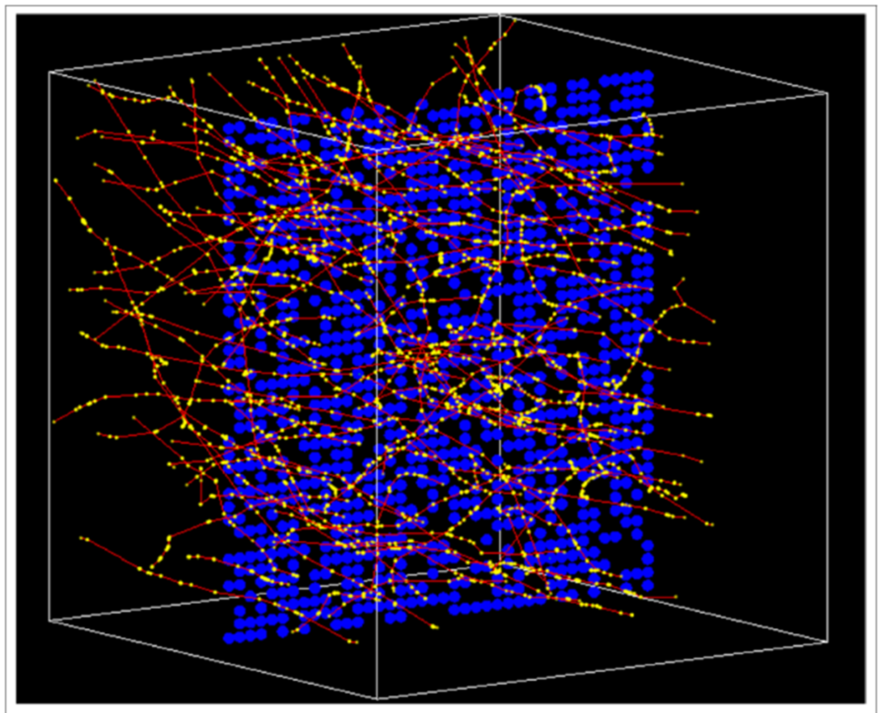
In simulation, we consider the direct radiation effect and indirect effect. The cell irradiation simulation is conducted using Geant4 [22]. The basic process of irradiation simulation using Geant4 is calculating the energy deposition points distribution information of all the cells. Then we calculate the cell dose and cell DSB number based on the energy deposition points information. Specifically, we use DBSCAN (Density-Based Spatial Clustering of Applications with Noise) algorithm [23, 24, 25] to obtain the DSB number of cells in the irradiation simulation. Also, we use a two-dimensional reaction-diffusion equation to quantify the bystander signal concentration in the cell culture, which is commonly adopted for modeling the diffusion and reaction process of bystander signals in the cell culture [26, 27].
The cell state transition process after irradiation within the simulated time is simulated. The cell phase distribution, cell state distribution, and cell survival fraction curve are obtained. At the starting time, the cell phase of each cell is randomly selected from five possible cell phases, i.e., G0, G1, S, G2, and M phase. In the simulation, the radiation is only delivered at the beginning time, . One simulation does not consider the radiation-induced bystander effect, while the other simulation considers the radiation-induced bystander effect. The total simulated time is 1667 minutes. The simulation parameters are listed in Table LABEL:tab:1.
| Name | Definition | Value | Unit | Reference |
| Dimension of cell culture in direction | 5 | mm | ||
| Dimension of cell culture in direction | 5 | mm | ||
| Dimension of cell home | 0.05 | mm | ||
| Time step for updating cell phase | 60 | second | ||
| Time step for updating cell state | 60 | second | ||
| Duration time of G1 phase | 15 | hour | Adopted from [28] | |
| Standard deviation of | 0.25 | hour | [8] | |
| Duration time of S phase | 9 | hour | Adopted from [28] | |
| Standard deviation of | 0.25 | hour | Adopted from [28] | |
| Duration time of G3 phase | 3 | hour | Adopted from [28] | |
| Standard deviation of | 0.25 | hour | Adopted from [28] | |
| Duration time of M phase | 1 | hour | Adopted from [28] | |
| Standard deviation of | 0.25 | hour | Adopted from [28] | |
| parameter for DSB number phase | 0.2497 | number | Estimated in this work, detailed estimation process seen in supplementary material | |
| parameter for integral number | 18.1517 | ml/pg | Estimated in this work, detailed estimation process seen in supplementary material | |
| Mean state energy of S1 state | 0 | Basis parameter, taking as zero | ||
| Mean state energy of S2 | 18.15 | Estimated in this work, detailed estimation process seen in supplementary material | ||
| Mean state energy of S3 | 48.47 | Estimated in this work, detailed estimation process seen in supplementary material | ||
| Standard deviation of state energy | 6.96 | Estimated in this work, detailed estimation process seen in supplementary material | ||
| Radiation sensivity factor of G1 phase | 1 | Basic parameter, taking as unit | ||
| Radiation sensivity factor of S phase | 0.816 | Extract the radiation sensitivity factors based on these published cell survival fraction curves. Here we take one published cell survival fraction curve in [29] | ||
| Radiation sensivity factor of G2 phase | 1.015 | Extract the radiation sensitivity factors based on these published cell survival fraction curves. Here we take one published cell survival fraction curve in [29] | ||
| Radiation sensivity factor of M phase | 1.015 | Extract the radiation sensitivity factors based on these published cell survival fraction curves. Here we take one published cell survival fraction curve in [29] | ||
| Fast decay constant of DSB | 3.31 | hour-1 | Adopted from [30] | |
| Slow decay constant of DSB | 0.14 | hour-1 | Adopted from [30] | |
| Weight fraction of fast decay of DSB | 0.62 | Adopted from [30] | ||
| Weight fraction of slow decay of DSB | 0.38 | Adopted from [30] | ||
| Total simulated time | 1667 | minute | ||
| Number of initial seeded cells | 1000 |
3 Results
3.1 Cell Phase Evolution
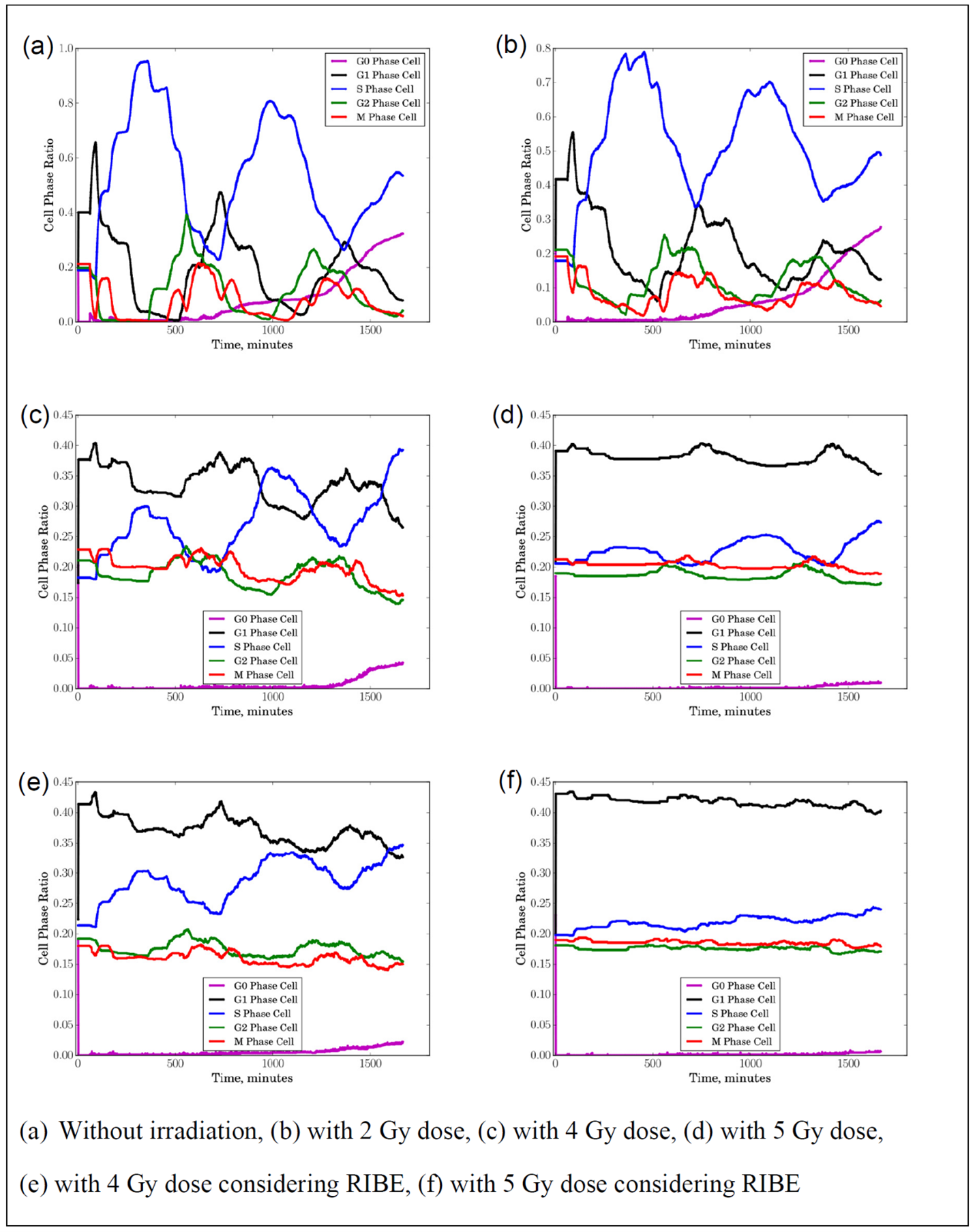
Figure 5a shows the cell phase distribution of 1000 seeded cells without irradiation. We can see that cells go through the normal proliferation process. With the initial cell phase distribution, the cell phase ratio of each cell phase varies with time. With cell phase progression, more and more cells will stay in quiescent state due to contact inhibition, so the cell phase of G0 increases. It is worth noting that the cell phase ratio distribution of interphase shows a periodic pattern reflecting the cell proliferation cycle. Figure 5b shows the cell phase distribution of seeded cells with 2 Gy dose irradiation, but no bystander effects are considered in the simulation. Compared to the condition of no irradiation, we can observe that the cell phase ratio of G1, S, and G2 all reduces due to radiation-induced cell death. Figure 5c shows the cell phase distribution of 1000 seeded cells with 4 Gy dose irradiation. We can see that there is a substantial decrease of cells going through mitosis and the periodic pattern of cell phase distribution in interphase is severely perturbed. Figure 5d shows the cell phase distribution of 1000 seeded cells with 5 Gy dose irradiation. We see that the cell phase distribution looks quite different compared to the case of no irradiation. Instead of a periodic pattern of cell phase ratio of interphase, the cell phase distribution has less variation with time because of fewer cells going through cell proliferation process. Figure 5e shows the cell phase distribution of 1000 seeded cells with 4 Gy dose irradiation, and bystander effects are considered in the simulation. We can see that there is a substantial difference in cell phase distribution between those simulations, and fewer cells going through mitosis compared to the case without considering bystander effects. We also can observe similar results for the simulation with 5 Gy dose irradiation as shown in Figure 5f.
3.2 Cell State Evolution
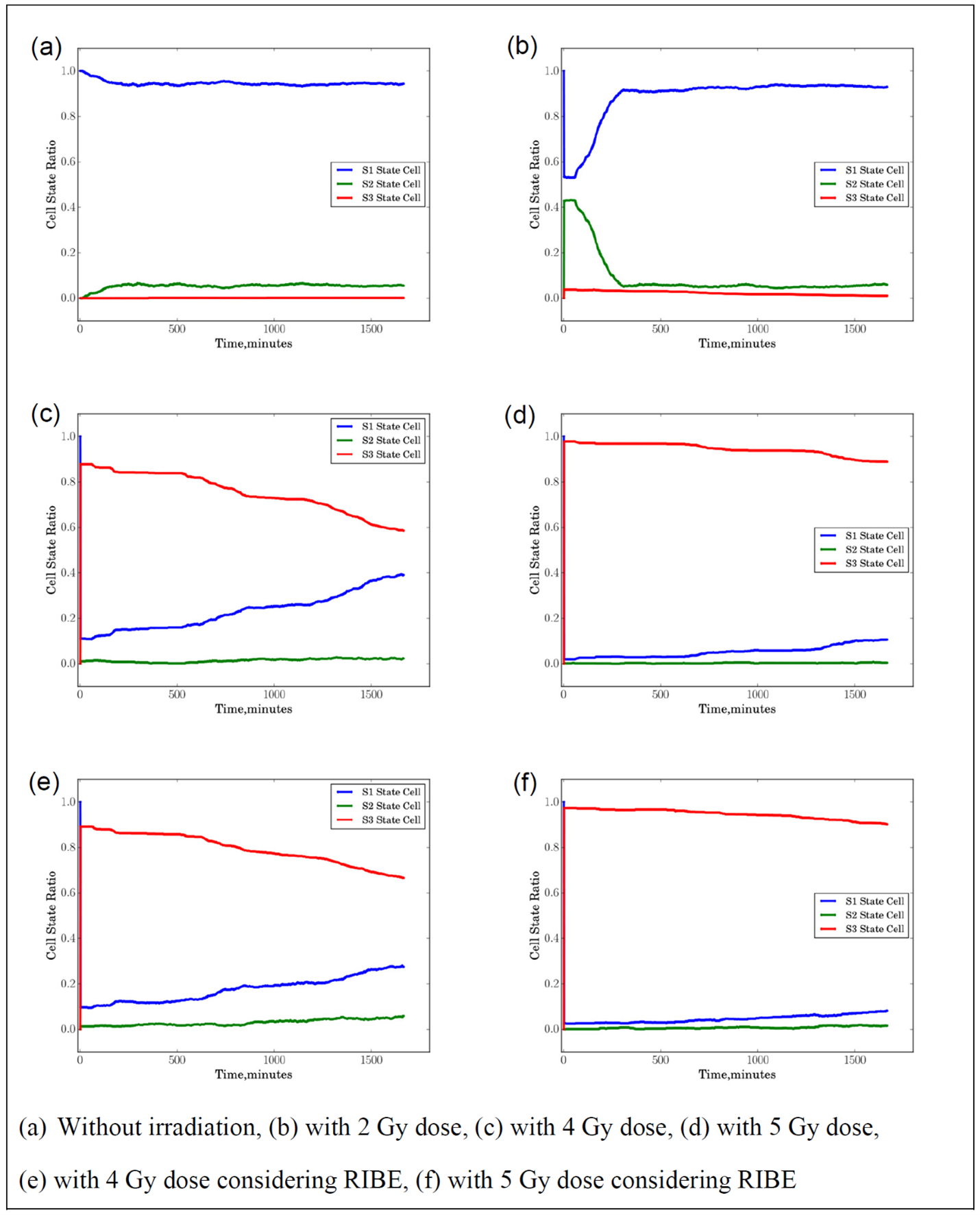
Figure 6a shows the cell state distribution of 1000 seeded cells without irradiation. For cells without irradiation, ideally, all the cells will stay in the healthy state S1 and the cell state distribution should be flat most of the time. However, due to the spontaneous death and spontaneous phase arrest, there are still some cells staying at S3 and S2 as shown in Figure 6a. Figure 6b shows the cell state distribution of 1000 seeded cells with 2 Gy dose irradiation. We can see that the ratio of S1 drops after the cell receives 2 Gy dose, while the ratio of S2 increases. The 2 Gy dose irradiation leads to cell death so the ratio of S1 has a drop after irradiation. Not all the cells are killed, so the with the cell proliferation and the damaged cells recovery the ratio of S1 gradually increases and saturates later. In contrast, with an initial increase, the ratio of S2 will gradually decrease and vary little with time going on. Figure 6c shows the cell state distribution of 1000 seeded cells with 4 Gy dose irradiation. We can see that the ratio of S1 substantially drops and the ratio of S3 increases after cell irradiation. Since there are still some surviving cells, the ratio of S1 gradually increases with time due to the newborn healthy cells and the ratio of S3 gradually decreases. Figure 6d shows the cell state distribution of 1000 seeded cells with 5 Gy dose irradiation. We can see that nearly 100% of cells are killed after irradiation, so the ratio of S3 increases after irradiation and varies little with time going on comparing to the case with 4 Gy irradiation, which means fewer cells go through proliferation after irradiation.
Figure 6e shows the cell state distribution of 1000 seeded cells with 4 Gy dose irradiation considering the bystander effects. We can see that fewer cells stay at S1 state considering the bystander effects compared to the case without considering bystander effects, but the difference is small, and it is less than 10% at most. We also can observe similar results for the simulation with 5 Gy dose irradiation as shown in Figure 6f.
3.3 Cell Survival Curve
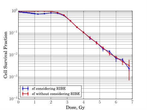
We obtained cell survival fraction curves of the seeded cells as shown in Figure 7. For the simulation case without modeling bystander effects, the cell survival curve captures the basic characteristics of survival fraction curve in experiment. There is a shoulder in the low dose region for the low LET radiation which is 1 MeV electron as simulated in this work, and there is an exponential drop when the dose passes the shoulder region. For the simulation case with modeling bystander effects, we also can observe that there is a hyper-radiosensitivity region when the dose is lower than 2 Gy.
4 Discussion
In this study, we introduce an agent-based simulation module (named Physical-Bio Translator) to simulate the cellular response after irradiation. The theoretical framework of the simulation is built upon a novel model, namely, the cell-state transition model, to simulate the cell’s response, which considers the realistic characteristics of irradiated cells. To validate the functionalities of the Physical-Bio Translator, we conducted an example simulation in which cell phase evolution, cell phenotype evolution, and cell survival were simulated. The results demonstrate that the Physical-Bio Translator can be used to replicate the cell irradiation experiment using simulation, showing promising prospects that a digital version of the cell irradiation experiment can be conducted through computer simulation with a better model for radiation biology. This work is a good start in paving the road for building a powerful and useful digital twin on multicellular or even tissue scales to study and predict patient responses to radiation therapy comprehensively.
Undoubtedly, the development of these digital twins will better promote the advancement of radiation biology, as digital twins can help us understand, observe, and even predict some radiation biology phenomena that traditionally require expensive and time-consuming experiments. Here, we use a discussion of the LQ model as an example to illustrate and support the ideas mentioned above, providing some initial insights to pave the way for further discussion.
A variety of cell survival models have been introduced to describe the cell survival data. The linear-quadratic (LQ) model is the most widely accepted mechanistic model of cell killing by radiation [31, 32, 33]. Despite its empirical nature, the LQ model is considered the best-fitting model to describe cell survival fraction curves and is of great interest in radiation oncology through radiotherapy-induced tissue reactions [34]. The LQ model stems from the curvilinear nature of dose response curves for the logarithm of cell survival. The binary misrepair model is the most common mechanistic rationale for the LQ formalism. However, to date, the LQ model still generates numerous debates, and inherent bio-molecular mechanisms remain unknown [34]. Besides the LQ model, some other models were also introduced, such as repair misrepair [35], the lethal-potentially lethal [36], or two-lesion kinetic model [37], etc. Overall, it is generally acknowledged that the biophysical basis of all such models rests on speculative assumptions about the microscopic events leading to the observed cell responses [26]. Moreover, these models also seem to lack a unified and logically coherent microscopic explanation for radiation biology. However, with the developed digital twin models, we can try to provide a more reasonable explanation for these models.
We simulate the cell survival fraction curve using the developed model without including any assumptions about the survival curve shape and lethal lesion distributions applied in the models. We obtained cell survival fraction curves of the seeded cells, and the results are in line with some experimental observations [38, 39, 40] where the hyper-radiosensitivity in the low dose region was reported. Thus, the simulated cell survival fraction curves suggest that the cell state transition theory is an effective theory to explore the radiation-induced effects from the first principles with limited hypotheses.
The key aim of developing this novel model is to overcome the inherent limitations of current traditional models, which lack a generalized theory for quantifying radiation-induced cellular effects, such as target effects and non-target effects. The model developed in this study has clear connections to physics and biology. Our developed model has parameters with direct biological meaning. Most importantly, these parameters can be quantified by experiment. The model developed in this work is a valuable tool for quantifying radiation-induced cellular effects, unraveling the intimate relationship between radiation energy deposition and biological effects.
To further improve this work, experimental validation of the bystander effect models introduced in this study is essential. Microbeam irradiation experiments targeting single cells or multicellular systems can provide direct evidence for validating the simulation results and the underlying mechanisms. Additionally, irradiation experiments using linear accelerators (linacs) with cultured cells can be employed to study cell viability, radiation-induced DNA damage repair kinetics, and other key biological endpoints. Such experimental validation would not only enhance confidence in the developed models but also provide insights into the applicability of the model to broader biological systems.
Another crucial aspect to consider is the uncertainty estimation of the model parameters. Accurate parameter estimation is critical for ensuring the predictive power and reliability of the simulation results. Future work should incorporate rigorous uncertainty quantification methods to account for variability in model parameters, providing a clearer understanding of their impact on the simulation outcomes.
5 Conclusions
In this study, we conducted a theoretical investigation to develop and implement a novel theory for quantifying radiation-induced cellular effects. This study is paired with new mathematical formalization and implementation methods for predicting the outcomes of cell responses after irradiation through an agent-based simulation method. We introduced a new set of mathematical structures for studying cell state transitions after irradiation, and the rigorous formalization ensures this mathematical structure remains well-posed and self-consistent. This resulted in a useful modeling theory for quantifying cell state transitions after irradiation, which serves as a key element for building an effective digital twin on a multicellular scale to simulate post-irradiation cellular responses. In the long run, this will serve as a crucial component of a digital twin framework for personalized radiation treatment.
6 Acknowledgments
RL acknowledges support from the Department of Radiation Oncology at the University of Nebraska Medical Center through faculty startup funding. Additional funding for this project was provided, in part, by The Otis Glebe Medical Research Foundation.
References
References
- [1] L. Bodgi, A. Canet, L. Pujo-menjouet, and A. Lesne, Mathematical models of radiation action on living cells: From the target theory to the modern approaches. A historical and critical review, J Theor Biol, vol. 394, pp. 93–101, 2016, doi: 10.1016/j.jtbi.2016.01.018.
- [2] D. J. Brenner, L. R. Hlatky, P. J. Hahnfeldt, Y. Huang, and R. K. Sachs, The linear-quadratic model and most other common radiobiological models result in similar predictions of time-dose relationships, Radiat Res, vol. 150, no. 1, pp. 83–91, 1998, doi: 10.2307/3579648.
- [3] S. B. Curtis, Lethal and potentially lethal lesions induced by radiation - a unified repair model, Radiat Res, vol. 106, no. 2, pp. 252–70, 1986, doi: 10.2307/3576798.
- [4] C. A. Tobias, The repair-misrepair model in radiobiology: comparison to other models, Radiat Res Suppl, vol. 8, no. May, pp. S77–S95, 1985.
- [5] R. D. Stewart, Two-lesion kinetic model of double-strand break rejoining and cell killing, Radiat Res, vol. 156, no. 4, pp. 365–78, Oct. 2001, Accessed: Jan. 17, 2016. [Online]. Available: http://www.ncbi.nlm.nih.gov/pubmed/11554848
- [6] N. Albright, A Markov Formulation of the Repair-Misrepair Model of Cell Survival, Radiat Res, vol. 118, no. 1, pp. 1–20, 1989.
- [7] M. P. Little, J. A. Filipe, K. M. Prise, M. Folkard, and O. V Belyakov, A model for radiation-induced bystander effects, with allowance for spatial position and the effects of cell turnover, J Theor Biol, vol. 232, no. 3, pp. 329–338, 2005, doi: 10.1016/j.jtbi.2004.08.016.
- [8] F. P. Faria, R. Dickman, and C. H. C. Moreira, Models of the radiation-induced bystander effect, Int J Radiat Biol, vol. 88, no. 8, pp. 592–9, Aug. 2012, doi: 10.3109/09553002.2012.692568.
- [9] A. Jansson, M. Harlen, S. Karlsson, P. Nilsson, and M. Cooley, 3D computation modelling of the influence of cytokine secretion on Th-cell development suggests that negative selection (inhibition of Th1 cells) is more effective than positive selection by IL-4 for Th2 cell dominance, Immunol Cell Biol, vol. 85, no. 3, pp. 189–96, Jan. 2007, doi: 10.1038/sj.icb.7100023.
- [10] Z. Nikitaki et al., Systemic mechanisms and effects of ionizing radiation: A new ‘old” paradigm of how the bystanders and distant can become the players, Semin Cancer Biol, Feb. 2016, doi: 10.1016/j.semcancer.2016.02.002.
- [11] J. Von, N. Sujnjnary, and G. E. Forsythe, Various Techniques Used in Connection With Random Digits, National Bureau of Standards, Applied Math Series, no. 12, pp. 36–38, 1951.
- [12] A. Asaithamby and D. J. Chen, Cellular responses to DNA double-strand breaks after low-dose gamma-irradiation, Nucleic Acids Res, vol. 37, no. 12, pp. 3912–23, Jul. 2009, doi: 10.1093/nar/gkp237.
- [13] P. M. Sharma, B. Ponnaiya, M. Taveras, I. Shuryak, H. Turner, and D. J. Brenner, High throughput measurement of H2AX DSB repair kinetics in a healthy human population, PLoS One, vol. 10, no. 3, p. e0121083, Jan. 2015, doi: 10.1371/journal.pone.0121083.
- [14] L. Herr, I. Shuryak, T. Friedrich, M. Scholz, M. Durante, and D. J. Brenner, New Insight into Quantitative Modeling of DNA Double-Strand Break Rejoining, Radiat Res, vol. 184, no. 3, pp. 280–95, Sep. 2015, doi: 10.1667/RR14060.1.
- [15] R. Hirayama, Y. Furusawa, T. Fukawa, and K. Ando, Repair kinetics of DNA-DSB induced by X-rays or carbon ions under oxic and hypoxic conditions, J Radiat Res, vol. 46, no. 3, pp. 325–332, 2005, doi: 10.1269/jrr.46.325.
- [16] F. Tommasino, T. Friedrich, U. Scholz, G. Taucher-Scholz, M. Durante, and M. Scholz, A DNA double-strand break kinetic rejoining model based on the local effect model, Radiat Res, vol. 180, no. 5, pp. 524–38, Nov. 2013, doi: 10.1667/RR13389.1.
- [17] G. Iliakis, Y. Wang, J. Guan, and H. Wang, DNA damage checkpoint control in cells exposed to ionizing radiation, Oncogene, vol. 22, no. 37, pp. 5834–5847, 2003, doi: 10.1038/sj.onc.1206682.
- [18] M. Mitchell, Computation in Cellular Automata: A Selected Review, Non-Standard Computation, pp. 95–140, 1998, doi: 10.1002/3527602968.ch4.
- [19] B. V Bronk, G. J. Dienes, and A. Paskin, The stochastic theory of cell proliferation, Biophys J, vol. 8, no. 11, pp. 1353–98, Nov. 1968, doi: 10.1016/S0006-3495(68)86561-0.
- [20] H. Kempf, H. Hatzikirou, M. Bleicher, and M. Meyer-hermann, In Silico Analysis of Cell Cycle Synchronisation Effects in Radiotherapy of Tumour Spheroids, PLoS Comput Biol, vol. 9, no. 11, 2013, doi: 10.1371/journal.pcbi.1003295.
- [21] M. Hwang, M. Garbey, S. A. Berceli, and R. Tran-Son-Tay, Rule-based simulation of multi-cellular biological systems-a review of modeling techniques, 2009. doi: 10.1007/s12195-009-0078-2.
- [22] S. Agostinelli et al., GEANT4 - A simulation toolkit, Nucl Instrum Methods Phys Res A, vol. 506, no. 3, pp. 250–303, Jul. 2003, doi: 10.1016/S0168-9002(03)01368-8.
- [23] J. Sander, M. Ester, H.-P. Kriegel, and X. Xu, A Density-Based Algorithm for Discovering Clusters in Large Spatial Databases with Noise, Data Min Knowl Discov, vol. 2, no. 2, pp. 169–194, 1998, doi: 10.1023/A:1009745219419.
- [24] Z. Francis, C. Villagrasa, and I. Clairand, Simulation of DNA damage clustering after proton irradiation using an adapted DBSCAN algorithm, Comput Methods Programs Biomed, vol. 101, no. 3, pp. 265–270, 2011, doi: 10.1016/j.cmpb.2010.12.012.
- [25] R. Liu, T. Zhao, M. H. Swat, F. J. Reynoso, and K. A. Higley, Development of Computational Model for Cell Dose and DNA Damage Quantification of Multicellular System, Int J Radiat Biol, pp. 1–14, Jul. 2019, doi: 10.1080/09553002.2019.1642537.
- [26] M. Tomezak, C. Abbadie, E. Lartigau, and F. Cleri, A biophysical model of cell evolution after cytotoxic treatments: damage, repair and cell response, J Theor Biol, vol. 389, pp. 146–158, 2015, doi: 10.1016/j.jtbi.2015.10.017.
- [27] Y. Hattori, A. Yokoya, and R. Watanabe, Cellular automaton-based model for radiation-induced bystander effects, BMC Syst Biol, vol. 9, no. 1, p. 90, Jan. 2015, doi: 10.1186/s12918-015-0235-2.
- [28] A. Altinok, D. Gonze, F. Le, and A. Goldbeter, An automaton model for the cell cycle, Interface Focus, vol. 1, no. November 2010, pp. 36–47, 2011.
- [29] E. J. Hall and A. J. Giaccia, Radiobiology for The Radiologist, 7th ed. 2012.
- [30] F. Tommasino, T. Friedrich, U. Scholz, G. Taucher-Scholz, M. Durante, and M. Scholz, A DNA double-strand break kinetic rejoining model based on the local effect model, Radiat Res, vol. 180, no. 5, pp. 524–38, Nov. 2013, doi: 10.1667/RR13389.1.
- [31] R. G. Dale, The application of the linear-quadratic dose-effect equation to fractionated and protracted radiotherapy, British Journal of Radiology, vol. 58, no. 690, pp. 515–528, 1985, doi: 10.1259/0007-1285-58-690-515.
- [32] A. M. Kellerer and H. H. Rossi, The theory of dual radiation action, Current topics in radiation research, vol. 8, pp. 85–158, 1972, doi: 10.1667/RRAV17.1.
- [33] D. E. Lea and D. G. Catcheside, The mechanism of the induction by radiation of chromosome aberrations in Tradescantia, J Genet, vol. 44, no. 2–3, pp. 216–245, Dec. 1942, doi: 10.1007/BF02982830.
- [34] L. Bodgi, A. Canet, L. Pujo-menjouet, and A. Lesne, Mathematical models of radiation action on living cells: From the target theory to the modern approaches. A historical and critical review, J Theor Biol, vol. 394, pp. 93–101, 2016, doi: 10.1016/j.jtbi.2016.01.018.
- [35] C. A. Tobias, The repair-misrepair model in radiobiology: comparison to other models, Radiat Res Suppl, vol. 8, no. May, pp. S77–S95, 1985.
- [36] S. B. Curtis, Lethal and potentially lethal lesions induced by radiation–a unified repair model, Radiat Res, vol. 106, no. 2, pp. 252–70, 1986, doi: 10.2307/3576798.
- [37] R. D. Stewart, Two-lesion kinetic model of double-strand break rejoining and cell killing, Radiat Res, vol. 156, no. 4, pp. 365–78, Oct. 2001.
- [38] C. Fernandez-Palomo, C. Seymour, and C. Mothersill, Inter-Relationship between Low-Dose Hyper-Radiosensitivity and Radiation-Induced Bystander Effects in the Human T98G Glioma and the Epithelial HaCaT Cell Line, Radiat Res, vol. 185, no. 2, pp. 124–33, 2016, doi: 10.1667/RR14208.1.
- [39] M. C. Joiner, B. Marples, P. Lambin, S. C. Short, and I. Turesson, Low-dose hypersensitivity: Current status and possible mechanisms, International Journal of Radiation Oncology Biology Physics, 2001, pp. 379–389. doi: 10.1016/S0360-3016(00)01471-1.
- [40] M. Tomita, K. Kobayashi, and M. Maeda, Microbeam studies of soft X-ray induced bystander cell killing using microbeam X-ray cell irradiation system at CRIEPI, J Radiat Res, vol. 53, no. 3, pp. 482–8, 2012, doi: 10.1269/jrr.11055.