\DeclareDelimFormat

[bib]multinamedelim, \DeclareDelimFormat[bib]finalnamedelim, \DeclareDelimFormat[parencite]nameyeardelim,

Deviations from the Nash equilibrium and emergence of tacit collusion in a two-player optimal execution game with reinforcement learning

Fabrizio Lillo^1,2¹¹1fabrizio.lillo@sns.it

and Andrea Macrì¹²²2andrea.macri@sns.it

¹ Scuola Normale Superiore, Pisa, Italy
² Dipartimento di Matematica University of Bologna, Bologna, Italy

(August 14, 2025)

Abstract

The use of reinforcement learning algorithms in financial trading is becoming increasingly prevalent. However, the autonomous nature of these algorithms can lead to unexpected outcomes that deviate from traditional game-theoretical predictions and may even destabilize markets. In this study, we examine a scenario in which two autonomous agents, modeled with Double Deep Q-Learning, learn to liquidate the same asset optimally in the presence of market impact, using the Almgren-Chriss (2000) framework. Our results show that the strategies learned by the agents deviate significantly from the Nash equilibrium of the corresponding market impact game. Notably, the learned strategies exhibit tacit collusion, closely aligning with the Pareto-optimal solution. We further explore how different levels of market volatility influence the agents’ performance and the equilibria they discover, including scenarios where volatility differs between the training and testing phases.

1 Introduction

The increasing automation of trading over the past three decades has profoundly transformed financial markets. The availability of large, detailed datasets has facilitated the rise of algorithmic trading—a sophisticated approach to executing orders that leverages the speed and precision of computers over human traders. By drawing on diverse data sources, these automated systems have revolutionized how trades are conducted. In 2019, it was estimated that approximately 92% of trading in the foreign exchange (FX) market was driven by algorithms as reported in [1]. The rapid advancements in Machine Learning (ML) and Artificial Intelligence (AI) have significantly accelerated this trend, leading to the widespread adoption of autonomous trading algorithms. These systems, particularly those based on Reinforcement Learning (RL), differ from traditional supervised learning models. Instead of being trained on labeled input/output pairs, RL algorithms explore a vast space of potential strategies, learning from past experiences to identify those that maximize long-term rewards. This approach allows for the continuous refinement of trading strategies, further enhancing the efficiency and effectiveness of automated trading.

The flexibility of RL comes with significant potential costs, particularly due to the opaque, black-box nature of these algorithms. This opacity can lead to unexpected outcomes that may destabilize the system they control—in this case, financial markets—through the actions they take, such as executing trades. The complexity and risk increase further when multiple autonomous agents operate simultaneously within the same market. The lack of transparency in RL algorithms may result in these agents inadvertently learning joint strategies that deviate from the theoretical Nash equilibrium, potentially leading to unintended market manipulation. Among the various risks, the emergence of collusion is particularly noteworthy. Even without explicit instructions to do so, RL agents may develop cooperative strategies that manipulate the market, a phenomenon known as tacit collusion. This type of emergent behavior is especially concerning because it can arise naturally from the interaction of multiple agents, posing a significant challenge to market stability and fairness.

In this paper, we investigate the equilibria and the emergence of tacit collusion in a market where two autonomous agents, driven by deep RL, engage in an optimal execution task. While tacit collusion in RL settings has been explored in areas such as market making (as reviewed below), much less is known about how autonomous agents behave when trained to optimally trade a large position. We adopt the well-established Almgren-Chriss framework first introduced in [2], for modeling market impact, focusing on two agents tasked with liquidating large positions of the same asset. The agents are modeled using Double Deep Q-Learning (DDQL) and engage in repeated trading to learn the optimal equilibrium of the associated open-loop game.

For this specific setup, the Nash equilibrium of the game has been explicitly derived in [3], providing a natural benchmark against which we compare our numerically derived equilibria. In addition, we explicitly derive the Pareto-optimal strategy and numerically characterize the Pareto-efficient set of solutions. Our primary goal is to determine whether the two agents, without being explicitly trained to cooperate or compete, can naturally converge to a collusive equilibrium, given the existence and uniqueness of the Nash equilibrium.

Our findings reveal that the strategies learned by the RL agents deviate significantly from the Nash equilibrium of the market impact game. Across various levels of market volatility, we observe that the learned strategies exhibit tacit collusion, closely aligning with the Pareto-optimal strategy. Given that financial market volatility is time-varying, we also examine the robustness of these strategies when trained and tested under different volatility regimes. Remarkably, we find that the strategies learned in one volatility regime remain collusive even when applied to different volatility conditions, underscoring the robustness of the training process.

Literature review.

Optimal execution has been extensively studied in the financial literature. Starting from the seminal contributions in [4] and in [2], many authors have contributed to extend the model’s consistency with reality. Notable examples in this area are: [5, 6, 7, 8, 9, 10, 11, 12, 13]. In its basic setting, the optimal execution problem considers just one agent unwinding or acquiring a quantity $q_{0}$ of assets within a certain time window. However, if many other agents are considered to be either selling or buying, thus pursuing their own optimal execution schedules in the same market, the model becomes more complicated since it now requires modelling other agents’ behaviour the same market. Using a large dataset of real optimal execution, [14] shows that the cost of an execution strongly depends on the presence of other agents liquidating the same asset. The increased complexity when treating the problem in this way allows for more consistency with reality and, at the same time, opens the path for further studies on how the agents interact with each other in such a context.

The optimal execution problem with $n$ -agents operating in the same market has thus been studied under a game theoretic lens in both its closed-loop (in [15, 16]) and open-loop (in [17, 18, 19, 3, 20]) formulations. In more recent works, rather than just optimal execution, liquidity competition is also analysed (as in [21, 22]) along with market making problems (as in [23, 24]).

In recent times, with the advancements of machine learning techniques, the original optimal execution problem has been extensively studied using RL techniques. Among the many³³3For a more comprehensive overview of the state of the art on RL methods in finance, please refer to [25] and [26], some examples in the literature on RL techniques applied to the optimal execution problem are found in [27, 28, 29].

Applications of multi-agent RL to financial problems are not incredibly numerous if compared to those that study the problem in a single agent scenario. Optimal execution in a multi-agent environment is tackled in [30], where the authors analyse the optimal execution problem form the standpoint of a many agents environment and an RL agent trading on Limit Order Book. The authors test and develop a multi-agent Deep Q-learning algorithm able to trade on both simulated and real order books data. Their experiments converge to agents who adopt only the so-called Time Weighted Average Price (TWAP) strategies in both cases. On the other hand, still on optimal execution problem’s applications of multi-agent RL, the authors in [31] analyse the interactions of many agents on their respective optimal strategies under the standpoint of cooperative competitive behaviours, adjusting the reward functions in the Deep Deterministic Policy Gradient algorithm used, in order to allow for either of the two phenomena, but still using the basic model introduced in [2], and modelling the interactions of the agents via full reciprocal disclosure of their rewards and not considering the sum of the strategies to be a relevant feature for the permanent impact in the stock price dynamics.

The existence of collusion and the emergence of collusive behaviours are probably the most interesting behaviours based on agents interaction in a market, as these are phenomena that might naturally arise in markets even if no instruction on how to and whether to collude or not, are given to the modelled agents. The emerging of tacit collusive behaviours has been analysed in various contexts. One of the first interesting examples is found in [32], where using Q-learning the authors show how competing producers in a Cournot oligopoly learn how to increase prices above Nash equilibrium by reducing production, thus firms learn to collude even if usually do not learn to make the highest possible joint profit. Hence the firms converge to a ‘collusive’ behaviour rather than to a ‘proper’ collusion equilibrium. Still in Cournot oligopoly, authors in [33] apply multi-agent Q-learning in electricity markets, the evidences of a collusive behaviour do still arise and the authors postulate that the collusive behaviour may arise from imperfect exploration of the agents in such a framework. Similarly, authors in [34] conclude that the use of deep RL leads to collusive behaviours faster than simulated tabular Q-learning algorithms. For what concerns financial markets, the problem becomes more involved since the actors in market do not directly set the price in a ‘one sided’ way as is the case for production economies that are studied in the previously cited works. Among the many contributions that study the emergence of collusive behaviours in financial markets, in [35] it is shown how tacit collusion arises between market makers, modelled using deep RL, in a competitive market. In [36] the authors show how market making algorithms tacitly collude to extract rents, and this behaviour strictly depends on tick size and coarseness of price grid. Finally, in [24] the authors use a multi-agent deep RL algorithm to model market makers competing in the same market, the authors show how competing market makers learn how to adjust their quotes, giving rise to tacit collusion by setting spread levels strictly above the competitive equilibrium level.

The paper is organised as follows: Section 2 introduces the market impact game theoretical setting, Section 3 introduces the DDQL algorithm for the multi-agent optimal execution problem, Section 4 discusses the results for different parameter settings, and finally, Section 5 provides conclusions and outlines further research directions.

2 Market impact game setting

The Almgren-Chriss model.

The setup of our framework is based on the seminal Almgren-Chriss model first introduced in [2] for optimal execution. In this setting, a single agent wants to liquidate an initial inventory of $q_{0}$ shares within a time window $[0,T]$ , which, in the discrete-time setting, is divided into $N$ equal time increments of length $\tau=T/N$ . The main assumption of the model is that the mid-price (or the efficient price) evolves according to a random walk with a drift depending on the traded quantity. Moreover, the price obtained by the agent differs from the mid-price by a quantity which depends on the quantity traded in the interval. More formally, let $S_{t}$ and $\tilde{S}_{t}$ be the mid-price and the price received by the agent at time $t$ , and let $v_{t}$ be the number of shares traded by the agent in the same interval; then the dynamics is given by

\displaystyle\begin{split}{S}_{t}&=S_{t-1}-g\left({v_{t}}/{\tau}\right)\tau+\sigma\tau^{\frac{1}{2}}\xi\\ \tilde{S_{t}}&={S}_{t-1}-h\left({v_{t}}/{\tau}\right)\end{split}

(1)

$S_{t}$ evolves because of a diffusion part $\xi\sim\mathcal{N}(0,1)$ multiplied by the price volatility $\sigma$ and a drift part, termed permanent impact, $g_{t}\left({v_{t}}/{\tau}\right)$ , assumed to be linear and constant: $g\left({v_{t}}/{\tau}\right)=\kappa{v_{t}}/{\tau}$ . The price $\tilde{S}_{t}$ received by the agent is equal to the mid-price $S_{t}$ but impacted by a temporary impact term also assumed to be linear and constant in time: $h(v_{t}/{\tau})=\alpha{v_{t}}/{\tau}$ .

The aim of the agent is to unwind their initial portfolio maximizing the cash generated by their trading over the $N$ time steps. This objective can be rewritten in terms of Implementation Shortfall (IS) that is defined in the single agent case as:

IS(\vec{v})=S_{0}q_{0}-\sum^{N}_{t=1}\tilde{S}_{t}v_{t}

(2)

where $\vec{v}=(v_{1},...,v_{N})^{\prime}\in{\mathbb{R}}^{N}$ is the vector containing the traded quantity in each time step. The optimisation problem of the agent can be written as

\min_{\vec{v}}\,\,\mathbb{E}[IS(\vec{v})]-{\lambda}\mathbb{V}[IS(\vec{v})]\leavevmode\nobreak\ \leavevmode\nobreak\ \leavevmode\nobreak\ \leavevmode\nobreak\ \leavevmode\nobreak\ s.t.\leavevmode\nobreak\ \leavevmode\nobreak\ \sum_{t=1}^{N}v_{t}=q_{0}

(3)

where $\lambda$ is the risk aversion parameter of the agent. Under the linearity assumption of the two impacts, the problem can be easily solved analytically. In the following, we are going to consider risk neutral agents ( $\lambda=0$ ) and in this case the optimal trading schedule is the TWAP, i.e. $v_{t}=q_{0}/N$ , where the trading velocity is constant.

Almgren-Chriss market impact game.

Now we consider two agents selling an initial inventory $q_{0}$ shares within the same time window time window $[0,T]$ . The traded quantities by the two agents in the time step $t$ are indicated with $v^{(1)}_{t}$ and $v^{(2)}_{t}$ and $V_{t}=v^{(1)}_{t}+v^{(2)}_{t}$ is the total quantity traded in the same interval. The equations for the dynamics are

\displaystyle\begin{split}{S}_{t}&=S_{t-1}-g\left({V_{t}}/{\tau}\right)\tau+\sigma\tau^{\frac{1}{2}}\xi\\ \leavevmode\nobreak\ \leavevmode\nobreak\ \tilde{S_{t}}^{(k)}&={S}_{t-1}-h\left({v^{(k)}_{t}}/{\tau}\right)\leavevmode\nobreak\ \leavevmode\nobreak\ \leavevmode\nobreak\ \leavevmode\nobreak\ \leavevmode\nobreak\ k=1,2\end{split}

(4)

i.e. the mid-price is affected by the total traded volume $V_{t}$ , while the price received by each agents depend on the quantity she trades.

Since more than one agent is optimising her trading and the cash received depends on the trading activity of the other agent, the natural setting to solve this problem is the one of game theory. Since each agent is not directly aware of the selling activity of the other agent and the two agents interact through their impact on the price process, the resulting problem is an open-loop game. The existence and uniqueness of a Nash equilibrium in such a symmetric open-loop game has been studied in [3] in the case of n different players and linear impact functions. First of all, the defined the Nash equilibrium as:

Definition 1 (Nash equilibrium ([3])).

In an $n$ players game, where $n\in\mathbb{N}$ , with $q^{(1)}_{0},\dots,q^{(n)}_{0}\in\mathbb{R}$ initial inventory holdings and $\lambda_{1},\dots,\lambda_{n}$ non-negative coefficients of risk aversion. A Nash equilibrium for mean-variance optimisation as in Eq. (3) is a collection of $\mathbf{q^{*}}=\{\vec{q}_{1}^{*},\dots,\vec{q}_{n}^{*}\}$ inventory holdings such that for each $k\in n,\leavevmode\nobreak\ {\vec{q}_{k}}\in\mathcal{A}_{\text{det}}$ the mean variance functional is minimised:

\mathbb{E}[IS(\vec{q}_{k}|\mathbf{q^{*}_{-k}})]-{\lambda_{k}}\mathbb{V}[IS(\vec{q}_{k}|\mathbf{{q}^{*}_{-k}})]

for each agent $k$ .⁴⁴4Where $\mathcal{A}_{\text{det}}$ is the set of all admissible deterministic trading strategies, for a more formal definition see [3]. Where $\mathbf{{q}^{*}_{-k}}$ are the strategies of the other players minus the strategy of the $k$ -agent that is being considered.

Then they proved that there exists a unique Nash equilibrium for the mean-variance optimisation problem. The unique Nash equilibrium strategy $q^{*(k)}_{t}$ , the Nash remaining inventory of agent $k$ at time $t$ , for $n$ players is given as a solution to the second-order system of differential equations:

\lambda^{(k)}\sigma^{2}q^{(k)}_{t}-2{\alpha}\tau\ddot{\,q}^{(k)}_{t}=\kappa\sum_{j\neq k}\dot{q}^{\,(k)}_{t}+{\alpha}\tau\sum_{j\neq k}\ddot{\,q}^{(k)}_{t}

(5)

with two-point boundary conditions

q^{(k)}_{0}=q_{0}\hskip 14.22636pt\text{and}\hskip 14.22636ptq^{(k)}_{T}=0\,\,,\hskip 14.22636pt\forall\,\,k=1,\dots,n

(6)

Focusing on the special case of two players, in [3] it is proved that the selling schedule at the unique Nash equilibrium is:

q^{*(1)}_{t}=\frac{1}{2}(\Sigma_{t}+\Delta_{t})\hskip 56.9055pt\text{and}\hskip 56.9055ptq^{*(2)}_{t}=\frac{1}{2}(\Sigma_{t}-\Delta_{t})

(7)

where:

\displaystyle\begin{split}\Sigma_{t}=V_{t}e^{-\frac{\kappa t}{6\alpha}}\frac{\sinh{\left(\frac{(N-t)\sqrt{\kappa^{2}+12\alpha\lambda\sigma^{2}}}{6\alpha}\right)}}{\sinh{\left(\frac{N\sqrt{\kappa^{2}+12\alpha\lambda\sigma^{2}}}{6\alpha}\right)}}\hskip 28.45274pt\text{and}\hskip 28.45274pt\Delta_{t}=V_{t}e^{\frac{\kappa t}{2\alpha}}\frac{\sinh{\left(\frac{(N-t)\sqrt{\kappa^{2}+4\alpha\lambda\sigma^{2}}}{2\alpha}\right)}}{\sinh{\left(\frac{N\sqrt{\kappa^{2}+4\alpha\lambda\sigma^{2}}}{2\alpha}\right)}}\end{split}

(8)

It can be noticed that the Nash inventory holdings, and thus the trading rates, now depend also on the permanent impact $\kappa$ , contrary to what happens in the single agent case studied in [2]. The open loop setting of the game excludes that the agents have knowledge of each others inventory holdings and, as said above, they interact only through the permanently-impacted price ${S}_{t}$ . The price level does not enter directly into the optimal inventory formula, but the permanent impact and the volatility of the asset on the other hand do, proportionally to agents’ risk aversion.

Beyond the Nash equilibrium.

In this setting, a Nash equilibrium exists and is unique. However, one could wonder if, apart from the Nash equilibrium, there are other solutions that might be non-Nash and collusive or, generally speaking, either better or sub-optimal, in terms of average costs obtained by either agent, when compared to the Nash solution. Motivated by this, we aim at studying how and under which conditions agents interacting in such an environment can adopt manipulative or collusive behaviours that consistently deviate from the Nash equilibrium. We use RL to train the agents to trade optimally in the presence of the other agent and we study the resulting equilibria. The aim is to ascertain whether while trading, sub-optimal or collusive cost profiles for either of the agents are attainable. In order to do so, we focus on the case where two risk neutral agents want to liquidate the same initial portfolio made by an amount $q_{0}$ of the same asset. We let the agents play multiple episode instances of the optimal execution problem in a multi-agent market. This means that, defining a trading episode to be the complete unwinding of the initial inventory $q_{0}$ over time $[0,T]$ in $N$ time steps by both agents, the overall game is made by iterated trades at each $t=1,\dots,N$ time-steps and by $B$ iterations of trading, each containing a full inventory liquidation episode. Each iteration is described by two vectors $\vec{v}^{\,(1)}_{(i)}$ and $\vec{v}^{\,(2)}_{(i)}$ containing the trading schedule of the two agents in episode $i$ . Moreover, each vector is associated with its IS, according to Eq. 2. We now define the set of admissible strategies and the average IS.

Definition 2.

In an iterated game with $B$ independent iterations, the set $\mathcal{A}$ of admissible selling strategies in iteration $i$ is composed by the pair of vectors $\vec{v}^{\,(1,2)}_{(i)}=(\vec{v}^{\,(1)}_{(i)},\vec{v}^{\,(2)}_{(i)})$ , such that for $k=1,2$ :

•

$\sum^{N}_{t=1}v^{(k)}_{(i),t}=q_{0}$
•

$\vec{v}_{(i),t}^{(k)}$ is $({\mathcal{F}}_{t})_{t\geq 0}$ - adapted and progressively measurable
•

$\sum^{N}_{t=1}(v^{(k)}_{(i),t})^{2}<\infty$

For any $\vec{v}^{\,(1,2)}_{(i)}\in\mathcal{A}$ the average Implementation Shortfall is defined as:

\bar{IS}(\vec{v}^{\,(1,2)}_{(i)})=\frac{1}{N}\sum^{N}_{t=1}IS(\vec{v}^{\,(1,2)}_{(i)},t)=IS(\vec{v}^{\,(1)}_{(i)})+IS(\vec{v}^{\,(2)}_{(i)})

(9)

Leveraging on [24] and [23], we define collusive strategies and we show that they are necessarily Pareto-optimal.

Definition 3 (Collusion).

In an iterated game with $B$ independent iterations, a pair of vectors of selling schedules $\vec{v}^{\,(1,2)}_{c}=(\vec{v}^{\,(1)}_{c},\vec{v}^{\,(2)}_{c})\,\,\in\mathcal{A}$ is defined to be a collusion if for each iteration $i$ and $\forall\,\,\vec{v}^{\,(1,2)}_{(i)}\in\mathcal{A}$ :

\bar{IS}(\vec{v}^{\,(1,2)}_{c})\leq\bar{IS}(\vec{v}^{\,(1,2)}_{(i)})

Definition 4 (Pareto Optimum).

In an iterated game with $B$ independent iterations, a pair of vectors of selling schedules $\vec{v}^{\,(1,2)}_{p}=(\vec{v}^{\,(1)}_{p},\vec{v}^{\,(2)}_{p})\,\,\in\mathcal{A}$ is a Pareto optimal strategy if and only if there does not exist $\vec{v}^{\,(1,2)}_{(i)}\in\mathcal{A}$ such that:

\displaystyle\begin{split}\forall\,\,i=1,\dots,M\,,\,\leavevmode\nobreak\ \leavevmode\nobreak\ \leavevmode\nobreak\ &\bar{IS}(\vec{v}^{\,(1,2)}_{p})\geq\bar{IS}(\vec{v}^{\,(1,2)}_{(i)})\\ \exists\,\,j=1,\dots,M\,,\leavevmode\nobreak\ \leavevmode\nobreak\ \leavevmode\nobreak\ &\bar{IS}(\vec{v}^{\,(1,2)}_{p})>\bar{IS}(\vec{v}^{\,(1,2)}_{(j)})\\ \end{split}

(10)

Proposition 1 (Collusive Pareto optima).

For an optimal execution strategy problem where two agents minimise costs as in Eq. (3) in a market as in Eq. (4), a collusive selling strategy $\vec{v}^{\,(1,2)}_{c}$ in the sense of Definition 3 is necessarily a Pareto optimum as defined in Definition 4. We call this a Collusive Pareto optimal strategy $\vec{v}^{\,(1,2)}_{cp}$ .

Proof.

By contradiction, suppose that $\vec{v}^{\,(1,2)}_{c}$ is not Pareto optimal, then there must exist an iteration $i$ and a strategy $\vec{u}^{\,(1,2)}_{(i)}=(\vec{u}^{\,(1)}_{(i)},\vec{u}^{\,(2)}_{(i)})$ such that:

\bar{IS}(\vec{u}^{\,(1,2)}_{(i)})\leq\bar{IS}(\vec{v}^{\,(1,2)}_{c})

(11)

But this contradicts the hypothesis that $\vec{v}^{\,(1,2)}_{c}$ is collusive and hence $\vec{v}^{\,(1,2)}_{c}$ must be Pareto-optimal. ∎

Having shown that a collusive strategy is in fact the Pareto-optimal strategy, we aim at finding the set of all Pareto-efficient strategies, i.e. those selling strategies that result in IS levels where it is impossible to improve trading costs for one agent without deteriorating the one of the other agent. These strategies are defined to be collusions in this game setup. We define the set of Pareto solutions and, within this set and we find the Pareto-optimum as the minimum within the set of solutions.

Definition 5 (Pareto-efficient set of solutions).

For a two-player game, with $B$ independent iterations and risk neutral players that aim to solve the optimal execution problem in a market model defined as in Eq. (4), the Pareto-efficient set of strategies is the set of strategies $\vec{v}^{\,(1,2)}$ such that the IS of one agent cannot be improved without increasing the IS value of the other agent.

We now provide the conditions that allows to find the set of Pareto-efficient solutions.

Theorem 1 (Pareto-efficient set of solutions).

The Pareto-efficient set of strategies are the solutions to the multi-objective optimisation problem:

\begin{cases}\min_{\vec{v}^{\,(1,2)}}\vec{f}\left(\vec{v}^{\,(1,2)}\right)\\ \text{s.t.}\,\,\{\vec{v}^{\,(1,2)}_{(i)}\in\mathcal{A},\,\,\vec{g}(\vec{v}^{\,(1,2)})=\vec{0}\}\end{cases}

(P1)

where:

\begin{split}\vec{f}(\vec{v}^{\,(1,2)})&=\left[\mathbb{E}\left(IS(\vec{v}^{\,(1)}|\vec{v}^{\,(2)})\right),\mathbb{E}\left(IS(\vec{v}^{\,(2)}|\vec{v}^{\,(1)})\right)\right]\\ \vec{g}(\vec{v}^{\,(1,2)})&=\left[\left(\sum^{N}_{t=1}v^{(1)}_{t}-q_{0}\right)\ ,\left(\sum^{N}_{t=1}v^{(2)}_{t}-q_{0}\right)\right]\end{split}

Proof.

Problem (P1) is a convex multi-objective optimisation problem with $n=N$ design variables $(\vec{v}^{\,(1,2)})$ , $k=2$ objective functions, and $m=2$ constraint functions. Leveraging on [37], in order to find the Pareto-efficient set of solutions, Problem (P1) can be restated in terms of Fritz-Johns conditions. We define the $\mathbf{L}\in{\mathbb{R}}^{(n+m)\times(k+m)}$ matrix as:

\mathbf{L}=\begin{bmatrix}\nabla_{\vec{v}^{\,(1,2)}}\vec{f}(\vec{v}^{\,(1,2)})&\nabla_{\vec{v}^{\,(1,2)}}\vec{g}(\vec{v}^{\,(1,2)})\\ \vec{0}&\vec{g}(\vec{v}^{\,(1,2)})\end{bmatrix}

(12)

then, the strategy $\vec{v}^{\,(1,2)}_{p}$ is a solution to the problem:

\mathbf{L}\cdot\vec{\delta}=\vec{0}

(P2)

where $\vec{\delta}=(\vec{\omega},\vec{\lambda})\in{\mathbb{R}}^{k+m}$ . Moreover, $\vec{v}^{\,(1,2)}_{p}$ is a Pareto-efficient solution if $\vec{\delta}$ exists, it is a non-trivial solution if $\vec{\delta}$ exists and $\vec{\delta}\neq\vec{0}$ .

Leveraging on [37], a solution $\vec{v}^{\,(1,2),*}$ to the Problem (P2) is a non-trivial Pareto-efficient solution if:

\det(\mathbf{L}(\vec{v}^{\,(1,2),*})^{T}\mathbf{L}(\vec{v}^{\,(1,2),*}))=\vec{0}

(13)

Where $\mathbf{L}(\vec{v}^{\,(1,2),*})$ denotes the matrix $\mathbf{L}$ where the argument of $F(\cdot)$ and $G(\cdot)$ functions is a strategy $\vec{v}^{\,(1,2),*}$ . Thus we say that a necessary condition for generic strategy $(\vec{v}^{\,(1,2),*})$ to be Pareto-efficient is to satisfy Eq. (13). In general, Eq. (13) gives the analytical formula that describes the Pareto-optimal set of solutions obtainable from Problem (P2). ∎

The analytical derivation of the Pareto-efficient set of strategies, i.e. of the Pareto-front, for this kind of problem is quite involved and cumbersome, although obtainable via standard numerical multi-objective techniques. Later in the paper, we will solve this problem numerically to find the set for the problem at hand. It is instead possible to derive the absolute minimum of the Pareto-efficient set of solutions since the problem is a sum of two convex functions and is symmetric. We call these strategies, one per agent, Pareto-optimal strategies in the spirit of Definition 4.

Theorem 2 (Pareto optimal strategy).

For a two-player game with $B$ independent iterations and risk-neutral players, the Pareto optimal strategy for all iterations $i$ defined as the solution of the problem:

\begin{cases}&\operatorname*{arg\,min}_{\vec{v}^{\,(1)},\vec{v}^{\,(2)}}\,\,F(\vec{v}^{\,(1,2)})\\ \text{s.t.}\hskip 28.45274pt&\left(\sum^{N}_{t=1}v^{(1)}_{t}-q_{0}\right)=0\\ &\left(\sum^{N}_{t=1}v^{(2)}_{t}-q_{0}\right)=0\end{cases}

(14)

where:

{F}(\vec{v}^{\,(1,2)})=\mathbb{E}\left(IS(\vec{v}^{\,(1)}|\vec{v}^{\,(2)})\right)+\mathbb{E}\left(IS(\vec{v}^{\,(2)}|\vec{v}^{\,(1)})\right)

(15)

is $\forall\,\,\,t=1,\dots,N$ and $\forall\,i=1,\dots M$ :

\begin{split}v^{\,(1)}_{t,p}=\frac{q_{0}}{N}\,\,,\hskip 56.9055ptv^{\,(2)}_{t,p}=\frac{q_{0}}{N}\end{split}

(16)

i.e. the TWAP strategy.

Proof.

Considering just an iteration $i$ of the two players’ game, we define $\vec{v}^{\,(1)}=\operatorname*{arg\,min}_{\vec{v}^{\,(1)}}IS(\vec{v}^{\,(1)}|\vec{v}^{\,(2)})$ , meaning that the strategy for agent $1$ is a function of the strategy of agent $2$ . And thus $\vec{v}^{\,(1)}$ the strategy that minimises the IS of agent $1$ given the strategy of agent $2$ . The same consideration holds for agent $2$ , where $\vec{v}^{\,(2)}=\operatorname*{arg\,min}_{\vec{v}^{\,(2)}}IS(\vec{v}^{\,(2)}|\vec{v}^{\,(1)})$ .

Leveraging on Proposition 1, the Pareto optimal strategies $\vec{v}^{\,(1)}_{p},\vec{v}^{\,(2)}_{p}$ of the agents considered solve:

\operatorname*{arg\,min}_{\vec{v}^{\,(1)},\vec{v}^{\,(2)}}\,\,F(\vec{v}^{\,(1,2)})

(P1)

where:

{F}(\vec{v}^{\,(1,2)})=\mathbb{E}\left(IS(\vec{v}^{\,(1)}|\vec{v}^{\,(2)})\right)+\mathbb{E}\left(IS(\vec{v}^{\,(2)}|\vec{v}^{\,(1)})\right)

(17)

we then set up a constrained optimisation problem, where the constraint binds the agents to just sell their initial inventory $q_{0}$ over the time window considered:

\begin{split}&\nabla_{\vec{v}^{\,(1,2)}}\left[{F}\left(\vec{v}^{\,(1,2)}\right)+\lambda_{1}\left(\sum^{N}_{t=1}v^{(1)}_{t}-q_{0}\right)+\lambda_{2}\left(\sum^{N}_{t=1}v^{(2)}_{t}-q_{0}\right)\right]=0\\ \end{split}

(18)

this can be decoupled into two distinct problems:

\begin{split}&\nabla_{\vec{v}^{\,(1)},\lambda_{1}}\mathcal{L}_{1}=\nabla_{\vec{v}^{\,(1)},\lambda_{1}}\left[\mathbb{E}\left(IS(\vec{v}^{\,(1)}|\vec{v}^{\,(2)})\right)+\lambda_{1}\left(\sum^{N}_{t=1}v^{(1)}_{t}-q_{0}\right)\right]=0\\ &\nabla_{\vec{v}^{\,(2)},\lambda_{2}}\mathcal{L}_{2}=\nabla_{\vec{v}^{\,(2)},\lambda_{2}}\left[\mathbb{E}\left(IS(\vec{v}^{\,(2)}|\vec{v}^{\,(1)})\right)+\lambda_{2}\left(\sum^{N}_{t=1}v^{(2)}_{t}-q_{0}\right)\right]=0\end{split}

(19)

Considering now just the first problem in the previous equation, we notice that:

\mathbb{E}\left(IS(\vec{v}^{\,(1)}|\vec{v}^{\,(2)})\right)=-\sum^{N}_{t=1}\kappa v^{\,(1)}_{t}\sum^{t}_{j=1}(v^{\,(1)}_{j}+v^{\,(2)}_{j})-\sum^{N}_{t=1}\alpha v^{\,(1)^{2}}_{t}

and thus, for every $t=1,\dots,N$ :

\begin{cases}&\frac{\partial\mathcal{L}_{1}}{\partial{v}^{\,(1)}_{t}}=-\kappa\left((2q_{0}-q^{\,(1)}_{t}-q^{\,(2)}_{t})+{v}^{\,(1)}_{t}\right)-2\alpha v^{\,(1)}_{t}+\lambda_{1}=0\\ &\frac{\partial\mathcal{L}_{1}}{\partial\lambda_{1}}=\left(\sum^{N}_{t=1}v^{(1)}_{t}-q_{0}\right)=0\end{cases}

(20)

where $\sum^{t}_{j=1}v^{\,(1)}_{j}=(q_{0}-q_{t})$ and $q_{t}$ is the level of inventory held at time-step $t=1,\dots,N$ , we notice that:

v^{\,(1)}_{t}=-\frac{\kappa(2q_{0}-q^{\,(1)}_{t}-q^{\,(2)}_{t})+\lambda_{1}}{\kappa+2\alpha}

thus:

\begin{split}0&=\sum^{N}_{t=1}-\frac{1}{\kappa+2\alpha}\kappa\left((2q_{0}-q^{\,(1)}_{t}-q^{\,(2)}_{t})+\lambda\right)-q_{0}\\ \lambda&=\frac{q_{0}(\kappa+2\alpha)}{N}+\kappa(2q_{0}-q^{\,(1)}_{t}-q^{\,(2)}_{t})\\ v^{\,(1)}_{t}&=-\frac{\kappa(2q_{0}-q^{\,(1)}_{t}-q^{\,(2)}_{t})}{\kappa+2\alpha}+\frac{q_{0}(\kappa+2\alpha)}{N(\kappa+2\alpha)}+\frac{\kappa(2q_{0}-q^{\,(1)}_{t}-q^{\,(2)}_{t})}{\kappa+2\alpha}\end{split}

Finally, the first and the last terms cancel out and we obtain that the Pareto-optimal strategy $\vec{v}^{\,(1)}_{p}$ is:

v^{\,(1)}_{t,p}=\frac{q_{0}}{N}\,\,\,\,,\,\,\forall\,\,\,t=1,\dots,N

(21)

for $v^{\,(2)}_{t,p}$ same considerations hold since the problem is symmetric.

∎

To study whether Collusive Pareto-optima or more generally non-Nash equilibria arise in this setting, we model the two agents by equally and simultaneously training them with RL based on Double Deep Q Learning (DDQL) algorithm where two agents interact in an iterative manner. We then analyse the results under the light of the collusion strategies derived above. The aim is to understand how and which equilibria will eventually be attained, and whether in attaining an equilibrium they tacitly collude in order to further drive the costs of their trading down. We will analyse their interactions in some limiting cases in order to study if and how the equilibrium found changes and adapts to the market dynamics in a model agnostic setting such as the DDQL algorithm.

3 Double Deep Q Learning for multi-agent impact trading

We model the algorithmic agents by using RL based on Double Deep Q-Learning (DDQL). The setup is similar to the single agent algorithm as in [27] and in [29], but now we consider two agents interacting in the same environment. Each agent employs two neural networks, namely the main Q-net ( $Q_{\text{main}}$ ) for action selection and the target Q-net ( $Q_{\text{tgt}}$ ) for state evaluation. The four nets are exactly the same and updated at exactly the same rate. The only difference between the two agents is the timing at which they act and the time at which their nets are updated. In fact, in a given time-step, the agent trading as second pays the price impact generated by the first one. To make the game symmetric, similarly to [20], at each time step a coin toss decides which agent trades first. This ensures the symmetry and guarantees that, as the game unfolds, no advantage in terms of trading timing is present for either of the two agents.

We divide the overall numerical experiment into a training and a testing phase. In the training phase we train both the agents to solve the optimal execution problem. In the testing phase, we employ what we learned in terms of $Q_{\text{main}}$ weights, letting the trained agents play an iterated trading game. All the results shown in Section 4 are obtained in the testing phase.

3.1 Setting of the numerical experiments

We consider two risk neutral agents whose goal is to unwind an initial position of $q_{0}=100$ shares with initial value $S_{0}=10\$$ within a time window $[0,T]$ . The window is divided into $N=10$ time-steps of length $T/N=\tau$ . The mid-price $S_{t}$ evolves as in Eq. (4), and the agents sell their whole inventory during the considered time-window. This is called an iteration and in order to train the DDQL algorithm we consider a number of $C$ iterations. This is called a run. Thus, a run of the game is defined to be an iterated game over both $N$ time-steps and in $C$ trading iterations.

Over the $C$ iterations, each agent learns how to trade via an exploration-exploitation scheme, thus using $\epsilon$ -greedy policies. This is obtained by changing the weights of their $Q_{\text{main}}$ net in order to individually choose the best policies in terms of rewards, related to the obtained IS. The scheme of the algorithm is thus symmetric, and for each agent it is divided into two phases: an exploration and an exploration phase managed by the parameter $\epsilon\in(0,1]$ , that is common to both the agents, that will decrease geometrically during training and globally initialised as $\epsilon=1$ . Depending on the phase, the way in which the quantities to sell $v_{t}$ are chosen changes, and it does so for each agent symmetrically. When the agents are exploring, they will randomly select quantities to sell $v_{t}$ in order to explore different states and rewards in the environment, alternatively, when the agents are exploiting, they will use their $Q_{\text{main}}$ net to select $v_{t}$ .

3.1.1 Action selection and reward function

For each of the $N$ time-steps and $C$ trading iterations, the agents’ knowledge of the state of market environment is the tuple $g^{i}_{t}=(t,q^{i}_{t},S_{t-1})$ for $i=1,2$ . Thus, each agent knows the current time-step, her individual remaining inventory, and the permanently impacted mid-price at the previous time step. Clearly, only the first and the last are common knowledge of the two agents, while no information on inventory $q_{t}$ or past selling actions $v_{t}$ is shared between the agents.

Then, depending on the current value of $\epsilon$ , a draw $\zeta$ , different for each agent, from a uniform distribution determines whether the agent performs exploration or exploitation. This means that with probability $\epsilon$ the agent chooses to explore and thus she chooses at time-step $t$ the quantity to sell $v_{t}$ sampling from a normal distribution with mean $\mu=\frac{q_{t}}{N-t}$ and standard deviation $\delta=|\frac{q_{t}}{N-t}|$ . In this way, on average we favour a TWAP execution, allowing for both positive and negative values of $v_{t}$ , meaning that sell and buy actions can be selected. In the exploration phase we bind the quantity to be sold to be $v_{i,t}\in[-q_{0},q_{0}],\,\,\,\,i=1,2$ . Alternatively, with probability $1-\epsilon$ , the agent chooses the optimal Q-action as the one that maximises the Q-values from $Q_{\text{main}}$ net, thus exploiting what learnt in the exploration phase. We bind the agents to sell all their inventory within the considered time window, still exploring a large number of states, rewards, and actions.

Once every $m$ actions taken during training iterations by both the agents, $\epsilon$ is multiplied by a constant $c<1$ such that $\epsilon\to 0$ as $m\to\infty$ . In this way, for a large number of iterations $C$ , $\epsilon$ converges to zero and the algorithm gradually stops exploring and starts to greedily exploit what the agent has learned in terms of weights $\theta$ of the $Q_{\text{main}}$ net. Notice that the update for $\epsilon$ happens at the same rate for both the agents, thus they explore and exploit contemporaneously, while the draw from the uniform distribution $\zeta$ is different for every agent. For each time step $t$ we decide which of the two agents trades first with a coin toss. Once that the ordering of the trades is decided, the action decision rule in the training phase unfolds as:

\displaystyle\begin{split}&\epsilon\in(0,1)\,\,,\,\,\zeta\sim\mathcal{U}(0,1)\\ &v_{t}=\begin{cases}\sim\mathcal{N}(\mu=\frac{q_{t}}{N-t},\delta=|\frac{q_{t}}{N-t}|)\,\,\,\,\,\,\,\,\,\,\,\,\,\,\,\,,\text{if}\,\,\zeta\leq\epsilon\\ \operatorname*{arg\,max}_{v^{\prime}\in[0,q_{t}]}Q_{M}(g^{i}_{t},v^{\prime}|\theta_{\text{main}})\,\,\,\,\,\,\,\,,\text{else}\end{cases}\end{split}

(22)

After this, each agent calculates the reward as:

r_{t,i}=S_{t-1}v_{t,i}-\alpha v^{2}_{t,i}\,\,\,\,\,,i=1,2

(23)

Notice that the actions of the other agent indirectly impact on the reward of the agent $i$ through the price $S_{t-1}$ , while nothing but the agent’s own actions are known in the reward.

Overall, the rewards for every $t\in[1,N]$ are:

\displaystyle\begin{split}r_{1,i}&=S_{0}v_{1,i}-\alpha v_{1,i}^{2}\\ r_{2,i}&=(S_{1}+\kappa(v_{1,i}+v_{1,i^{-}})+\xi)v_{2,i}-\alpha v_{2,i}^{2}\\ \vdots&\\ r_{N,i}&=(S_{N-1}+\kappa(v_{N-1,i}+v_{N-1,i^{-}})+\xi)v_{N,i}-\alpha v_{N,i}^{2}\\ \end{split}

(24)

Where by $i^{-}$ we denote the the other agent, assuming that we are looking at the reward for agent $i$ , and $\xi\sim\mathcal{N}(0,\sigma)$ .

Thus, for each time step $t$ the agent $i$ sees the reward from selling $v_{t,i}$ shares, and stores the state of the environment, $g_{t,i}$ , where the sell action was chosen along with the reward and the next state $g_{t+1,i}$ where the environment evolves. At the end of the episode, the reward per episode per agent is $-q_{0}S_{0}+\sum^{N}_{t=1}S_{t-1}v_{t,i}-\alpha v_{t,i}^{2}$ . Written in this form, the aim of the agent is to cumulatively maximise such reward, such that the liquidation value of the inventory happens as close as possible to the initial value of the portfolio.

3.1.2 Training scheme

Table 1: Fixed parameters used in the DDQL algorithm. The parameters not shown in the table change depending on the experiments and are reported accordingly.

DDQL parameters				Model parameters
NN layers	$5$	$C$ train its.	$5,000$	$N$ intervals	$10$
Hidden nodes	$30$	$M$ test its.	$2,500$	$S_{0}$ price	$10\$$
ADAM lr	$0.0001$	$m$ reset rate	$75$ acts.	$q_{0}$ inventory	$100$
Batch size $b$	$64$	$c$ decay rate	$0.995$	$\alpha$ t. impact	$0.002$
$L$ mem. len.	$15,000$	$\gamma$ discount	$1$	$\kappa$ p. impact	$0.001$

Bearing in mind that the procedure is exactly the same for both agents, we focus now on the training scheme of one of them, dropping the subscript $i$ . We let the states $g_{t}$ , actions $v_{t}$ , rewards $r_{t}$ and subsequent future states $g_{t+1}$ obtained by selling a quantity $v_{t}$ in state $g_{t}$ , to form a transition tuple that is stored into a memory of maximum length $L$ , we have two different memories, one for each agent. As soon as the memory contains at least $b$ transitions, the algorithm starts to train the Q-nets. To this end, the algorithm samples random batches of length $b$ from the memory of the individual agent, and for each sampled transition $j$ it individually calculates:

\displaystyle y^{j}_{t}(\theta_{\text{tgt}})=\begin{cases}r^{j}_{t}&\text{if }{t}=N;\\ r^{j}_{t}+\gamma Q_{\text{tgt}}(g^{j}_{t+1},v^{*}|\theta_{\text{tgt}})&\text{else}\end{cases}

(25)

In Eq. (25), $r^{j}_{t}$ is the reward for the time step considered in the transition $j$ , $g^{j}_{t+1}$ is the subsequent state reached in $t+1$ , known since it is stored in the same transition $j$ , while $v^{*}=\operatorname*{arg\,max}_{v}Q_{\text{main}}(g^{j}_{t},v|\theta_{\text{main}})$ . $\gamma$ is a discount factor that accounts for risk-aversion⁵⁵5We set a $\gamma=1$ since we model risk neutral agents. Each agent individually minimises the mean squared error loss between the target $y(\theta_{\text{tgt}})$ and the values obtained via the $Q_{\text{main}}$ net. In formulae:

{L}(\theta_{\text{main}},\theta_{\text{tgt}})=\frac{1}{b}\sum^{b}_{\ell=1}\left(\left[y^{\ell}_{t}(\theta_{\text{tgt}})-Q_{\text{main}}(g^{\ell}_{t},v^{\ell}_{t}|\theta_{\text{main}})\right]\right)^{2}

\theta^{*}_{\text{main}}=\operatorname*{arg\,min}_{\theta_{\text{main}}}\mathcal{L}(\theta_{\text{main}},\theta_{\text{tgt}})

We then use back propagation and gradient descent in order to update the weights of the $Q_{\text{main}}$ net. This procedure is repeated for each agent and for each random batch of transition sampled from the agent’s memory. Overall, once both agents have individually performed $m$ actions, we decrease $\epsilon$ by a factor $c<1$ and we set $Q_{\text{tgt}}=Q_{\text{main}}$

Once both agents have been simultaneously trained to optimally execute a quantity $q_{0}$ while interacting only through the midprice, we let the agents interact on another number $M<C$ of trading iterations. This is the testing phase, and now actions for each agent are selected using just her $Q_{\text{main}}$ net. As said above, the results analysed below are those obtained in the testing phase.

The features of the Q-nets for each agent are ( $q_{i,t},t,S_{t-1},v_{i,t}$ ) and are normalised in the domain $[-1,1]$ using the procedure suggested in [27], whereas normalised mid-prices $\bar{S}_{t}$ are obtained via min-max normalisation. In our setup we use fully connected feed-forward neural networks with $5$ layers, each with $30$ hidden nodes. The activation functions are leakyReLu, and finally we use ADAM for optimisation. With the exception of the volatility parameter $\sigma$ which will be specified later, the parameters used in the algorithm are reported in Table 1, the training algorithm is reported in Algorithm 1.

Algorithm 1 Training of Double Deep Q-Learning multi-agent impact game

Set

\epsilon=1

b

batch size,

C

train iterations;

Set market dynamics parameters;

For each agent

i=1,2

initialise with random weights

Q_{\text{main}}

and make a copy

Q_{\text{tgt}}

;

For each agent

i=1,2

initialise the memory with max length

L

for k in C do

Set

S^{k}_{0}=S_{0}

;

for t in N do

u\sim\text{Bin}(1,0.5)

;

\triangleright

Decides the order of execution

u=0

then

i=(1,2)\,\,\,\text{else}\,\,\,i=(2,1)

end if

\triangleright

Vector of priority ordering of the agents

for each agent

i

in the order decided above do

g_{i,t}\leftarrow(q_{i,t},t,S^{k}_{t})

;

v_{i,t}\leftarrow\begin{cases}\text{sample}\,\,\,\mathcal{N}(\mu=\frac{q_{t}}{N-t},\delta=|\frac{q_{t}}{N-t}|)\,\,\,\,\,\,\,\,\,\,\,\,\,\,\,\,,\text{with probability $\epsilon$}\\ \operatorname*{arg\,max}_{v^{\prime}\in[0,q_{t}]}Q_{M}(g_{t},v^{\prime}|\theta_{\text{main}})\,\,\,\,\,\,\,\,,\text{with probability ($1-\epsilon$)}\end{cases};

r_{t}\leftarrow S^{i}_{t-1}v_{t}-\alpha v^{2}_{t}

;

S^{k}_{t-1}\to S^{k}_{t}

;

\triangleright

Generate

S^{k}_{t}

from

S^{k}_{t-1}

g_{i,t+1}\leftarrow(q_{i,t+1},t+1,S^{k}_{t})

;

Memory for agent

i

\leftarrow(g_{i,t},r_{i,t},v_{i,t},g_{i,t+1})

;

\triangleright

Memory storing

if Length of memory

\geq

b

then

for j in

b

Sample a batch of

(g^{j}_{i,t},r^{j}_{i,t},v^{j}_{i,t},g^{j}_{i,t+1})

from memory;

v^{*}_{i}=\operatorname*{arg\,max}_{v}Q_{i,\text{main}}(g^{j}_{i,t},v^{j}_{i,t}|\theta_{i,\text{main}})

;

y^{j}_{i,t}(\theta_{i,\text{tgt}})=\begin{cases}r^{j}_{i,t}&\text{if }{t}=N;\\ r^{j}_{i,t}+\gamma Q_{i,\text{tgt}}(g^{j}_{i,t+1},v^{*}_{i}|\theta_{i,\text{tgt}})&\text{else}\end{cases}

end for

\theta^{*}_{i,\text{main}}=\operatorname*{arg\,min}_{\theta_{i,\text{main}}}\mathcal{L}(\theta_{i,\text{main}},\theta_{i,\text{tgt}})

via gradient descent with loss to minimise:

{L}(\theta_{i,\text{main}},\theta_{i,\text{tgt}})=\frac{1}{b}\sum^{b}_{\ell=1}\left(\left[y^{\ell}_{t}(\theta_{i,\text{tgt}})-Q_{i,\text{main}}(g^{\ell}_{i,t},v^{\ell}_{i,t}|\theta_{i,\text{main}})\right]\right)^{2}

if Length of agent

i

memory =

L

then halve the length of agent

i

memory

end if

After

m

iterations decay

\epsilon=\epsilon\times c

;

After

m

iterations

\theta_{i,\text{tgt}}\leftarrow\theta_{i,\text{main}}

;

end for

Refer to caption — Figure 1: Scatter plot of the IS of the two agents for 20 testing runs of 2500 iterations in the zero noise case ( $\sigma=10^{-9}$ ).

4 Results

In this Section we present the results obtained by using the RL Algorithm 1 in the game setting outlined in Section 2. The experiments aim at studying the existence and the form of the learnt equilibria, by analysing the policies chosen by the two interacting trading agents. We then compare the equilibria with the Nash equilibrium, the Pareto-efficient set of solutions, and the Pareto optimal strategy. We consider different scenarios, using the market structure as outlined in Eq. (4).

It can be easily noticed how the theoretical Nash equilibrium for this game does not depend on the volatility level of the asset. In fact, when the risk aversion parameter $\lambda=0$ , the Nash equilibrium of Eq. (7) depends only on the permanent and temporary impact coefficients $\kappa$ and $\alpha$ , respectively. However, in the numerical determination of the equilibrium solution, volatility $\sigma$ and the associated diffusion play the role of a disturbance term, since an agent cannot determine whether an observed price change is only due to the impact generated by the trading of the other agent or if it is a random fluctuation due to volatility. In this sense, volatility plays the role of a noise-to-signal ratio here. To quantify the effect of volatility on the learnt equilibria, we perform three sets of experiments for different levels of the volatility parameter $\sigma$ , leaving unchanged the impact parameters. More specifically we consider, for both training and testing phase the case where $\sigma=10^{-9}$ (termed zero noise case), $\sigma=10^{-3}$ (moderate noise) and $\sigma=10^{-2}$ (large noise) case. In all three cases, we use the same temporary and permanent impacts $\alpha=0.002$ and $\kappa=0.001$ .

We employ 20 training and testing runs, each run is independent from the others, meaning that the weights found in one run are not used in the others. In this way we aim at independently (run-wise) train the agents to sell their inventory. Each testing run has $M=2,500$ iterations of $N=10$ time-steps.

4.1 The zero noise case

When $\sigma=10^{-9}$ we model the interaction of both agents in a limiting situation when the market is very illiquid and almost no noise traders enter the price formation process. In this case, the permanent impact is essentially the only driver of the mid-price dynamics in Eq. (4), thus price changes are triggered basically only by the selling strategies used by the agents throughout the game iterations.

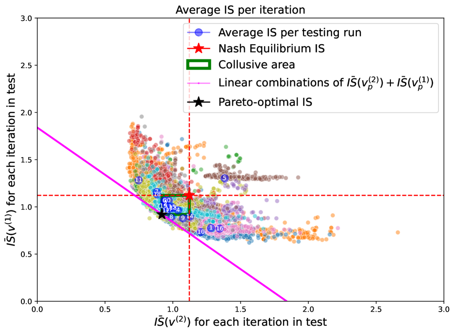
The results of the experiments are displayed in Figure 1, which shows, as a scatter plot, the $IS$ of both agents in each iteration of the testing phase. Each colour represents the results of one of the $20$ runs of $2,500$ iterations each. The blue circles shows the $IS$ centroids per testing run (the number in the circle identifies the run). For comparison the plot reports as a red star the point corresponding to the Nash equilibrium of Eq. (7), which is used to divide the graph into four quadrants, delimited by the red dashed lines. The top-right quadrant contains point which are sub-optimal with respect to the Nash equilibrium for both players, while the points in the top-left and bottom-right quadrant report points where the found equilibrium favours one of the two agents at the expenses of the other. In particular, in these regions one of the agents achieve an IS smaller than the one of the Nash equilibrium, while the other agents performs worst. In a sense, one of the agents predates on the other in terms of reward. The bottom-left quadrant is the most interesting, since here both agents are able to achieve an $IS$ smaller than the one in the Nash equilibrium and thus contain potential collusive equilibria. For comparison, the black star indicates the $IS$ of the Pareto-optimal strategy found in Theorem 2, while the magenta line is the linear combination of the Pareto-optimal $IS$ . Finally, the green rectangle denotes the area between the Nash and the Pareto-optimal $IS$ s, and we call it the collusive area. In fact, in that area we find the $IS$ s for both the agents that lie between the proper collusion defined by the Pareto-optimum and the Nash equilibrium.

Looking at Figure 1 we can notice that the $IS$ s per testing run concentrate in the collusive area of the graph (green rectangle) between the Nash and the Pareto-optimal $IS$ . This means that when the noise is minimal, it is easier for the agents to adopt tacit collusive behaviour and obtain costs that fall near the collusion $IS$ , i.e. the Pareto-optimum. The majority of the remaining $IS$ s per iteration still lie within the second and fourth quadrant of the graph, meaning that again they are in general able to find strategies that, at each iteration, do not allow one agent to be better without worsening the other.

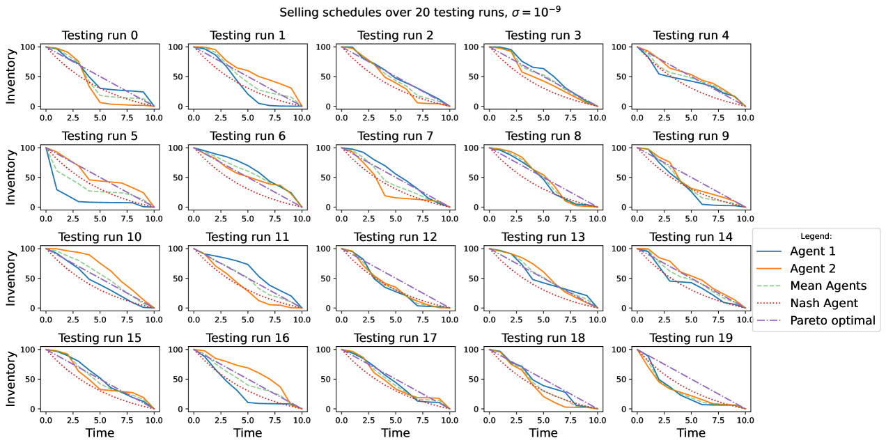
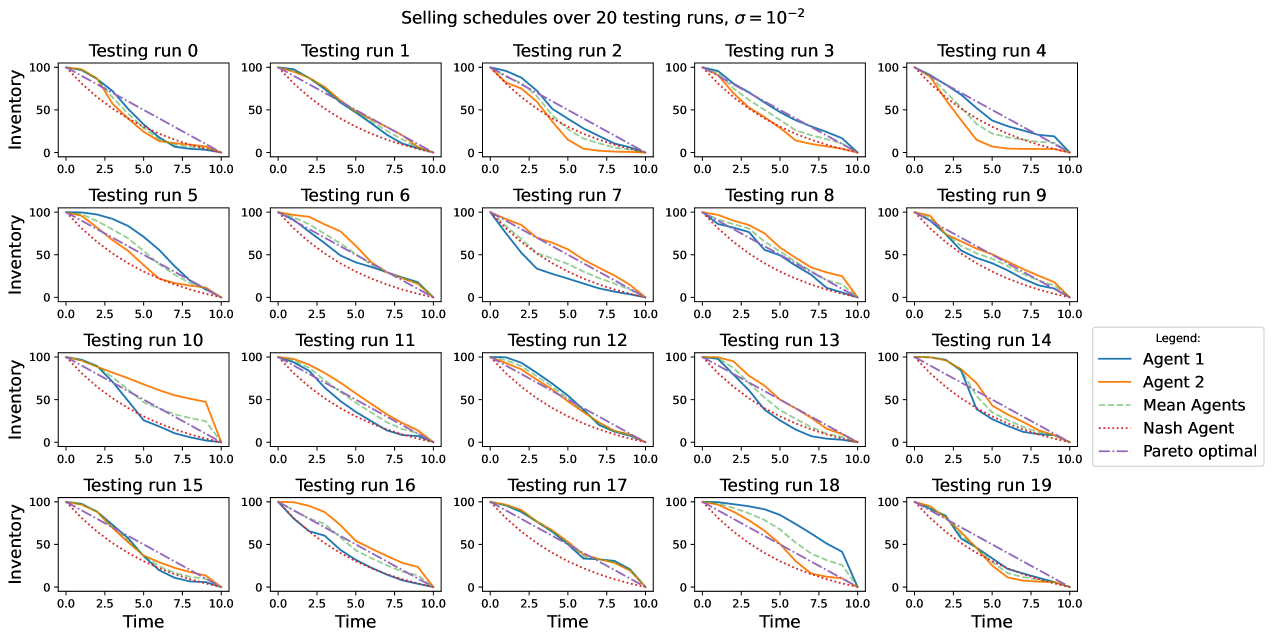
Considering the strategies found by the agents in Figure 2, we notice how the agents keep on trading at different speed, i.e. their selling policies are consistent with the presence of a slow trader and a fast trader. It can be seen how the policies followed by the agents in almost all the 20 simulations depend inversely on the strategy adopted by the competitor. Moreover, in most of the runs in the collusive region, the average strategy of the agents is very similar to the TWAP strategy. This is possible thanks to very low noise, and in this case the agents are able to find more easily the Pareto-optimal strategy, which corresponds to an equilibrium where they both pay the lowest amount possible in terms of $IS$ by tacitly colluding with their trading.

These evidences underline the quite intuitive fact that, when the noise to signal ratio is low it is simple for the agents to disentangle their actions from those of other agents. The agents find an incentive to deviate from the Nash-equilibrium adopting strategies that allow for lower costs. The majority of these strategies correspond to an average collusive $IS$ s, thus with lower cost than in the Nash equilibrium, but still slightly greater than the Pareto-optimum in terms of $IS$ s. In general, per iteration neither agent can be better off without increasing the other agent cost level. There is thus a strong evidence of tacit collusion, which in turn substantiates in the way the agents trade at different speeds. The phenomenon is evident thanks to the very low level of asset’s volatility. Thus, evidences of tacit collusive behaviour in this first case exist, moreover the collusive behaviour is adopted by the agents even if they have neither information about the existence nor about the strategy of the other agent trading in the market.

4.2 The moderate noise case

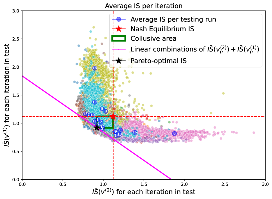
In this setting, the mid-price dynamics is influenced both by the trading of the agents and by the volatility. The first thing that can be noticed in Figure 3 is that the $IS$ per iteration distributes almost only in the second, third and fourth quadrant of the plot. Moreover, the distribution of the points suggests an inverse relation between the $IS$ s of the two agents, i.e. a lower $IS$ of an agent is typically associated with a worsening of the $IS$ of the other agent. The centroids distribute accordingly. In fact, the centroids that lie in the collusive area of the graph are as numerous as those that lie outside of that area on either the second or fourth quadrant. It can be seen that, outside the green rectangle, the agents tend to behave in a predatory way, meaning that one agent has consistently lower costs than the other. This happens tacitly, meaning that no information about the existence or about the strategy followed by the other agent is part of the information available either in the market or in each agent’s memory. Notice that predatory strategies are still consistent with the definition of Pareto efficiency but are not a proper collusion since they do differ from the Pareto-optimal $IS$ , even if they appear to overlap in Figure 3.

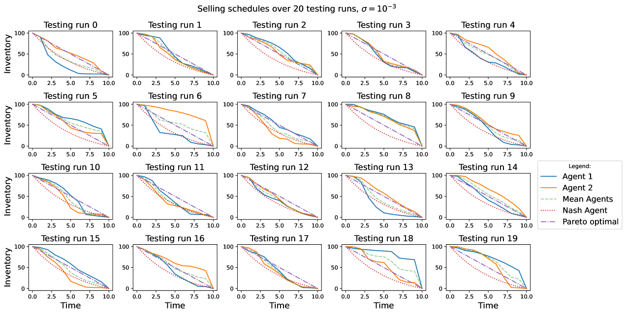
Looking at the average strategies implemented by the agents in each testing run (Figure 4), it can be noticed how similarly as in the zero noise case, roughly speaking there is almost always one agent that trades faster than the other and again as in the previous case, the one agent that trades slower is the one with an higher $IS$ . The comparison of Figure 4 and Figure 3shows that the agent that ‘predates’ the other is a fast trader and obtains lower costs of execution. This behaviour is more pronounced in this case, and we postulate that this is due to the increased level of noise for this experiment.

We conclude once again that, even if no explicit information about the trading strategies is shared by the agents, during the repeated game they are able to extrapolate information on the policy pursued by the competitor through the changes in the mid-price triggered by their own trading and by the other agent’s trading. Thus, it seems plausible that RL-agents modelled in this way are able to extrapolate information on the competitor’s policy and tacitly interact through either a collusive behaviour that leads to lower costs, either for both or for just one of them, resulting in a predatory behaviour or through a predatory behaviour where the costs of one agent are consistently higher than those of the other. Generally speaking, the set of solutions achieved is in line with the definition of the Pareto efficient set of solutions.

4.3 The large noise case

Finally, we study the interactions between the agents when the volatility of the asset is large. This corresponds to a relatively liquid market, since price changes are severely affected by the volatility level. Looking at Figure 5, we notice that in this market setup the higher level of volatility significantly affects the distribution of the $IS$ per iteration. In fact, the points in the scatter plot now distribute obliquely, even if for the most part they still lie in the second, third, and fourth quadrants. Because of the higher volatility level, very low $IS$ values for both agents might be attained per iteration and the structure of the costs per iteration is completely different with respect to to the previous cases. However, the distribution of the average $IS$ s per testing run, i.e. the positions of the centroids, is still concentrated for the greatest part in the collusive strategies area in between the Pareto-optimum and the Nash equilibrium costs.

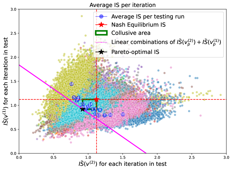
Figure 6 shows the trading strategies for the agents. It can still be noticed how in general if one agent is more aggressive with its trading, the other tends to be not. This tacit behaviour of the agents resulting in faster and slower traders still takes place, and again the agent that is trading slower pays more in terms of $IS$ , hence coupling the centroids’ distribution and the selling schedules in Figure 6 and Figure 5 reveals how a slower trading speed worsens the cost profile of one agent to the benefit of the other. The average trading strategy of the agents per testing run in the collusive cases basically revolves around a TWAP strategy that is in turn the Pareto-optimum for the considered problem.

4.4 Summary of results and comparison with the Pareto front

We have seen above that especially in the presence of significant volatility, the points corresponding to the iterations of a run tend to distribute quite widely in the scatter plot. The centroid summarises the average behaviour in a given run and provides a much more stable indication of the relation between the $IS$ of the two agents. To have a complete overview of the observed behaviour across the three volatility regimes, in Figure 7 we show in a scatter plot the position of the centroids of the $20\times 3$ testing runs. It can be seen that the centroids tend to concentrate in the collusive area, irrespective of the volatility level for the experiment. We notice how the agents’ costs tend to cluster in this area and to be close to the Pareto-optimal $IS$ . To have a more detailed comparison of the simulation results with the theoretical formulation of the game, we numerically compute the Pareto-efficient set of solutions (or Pareto-front)⁶⁶6The numerical Pareto front has been obtained using ‘Pymoo’ package in Python introduced in [38]. of and represent it on the scatter plot. The Figure shows that, as expected, the centroids lie on the right of the front. More interestingly, they are mostly found between the front and the Nash equilibrium for all the levels of volatility and, in line with the definition of the Pareto-front, for an agent to get better the other has to be worse off. We further notice that the majority of points for the zero noise case lies very close the Pareto optimum or in the collusive area, thus the lower the volatility the easier it is to converge to the collusion strategy. In the other two cases we notice how, even roughly half of the centroids lie in the collusive area, the rest mostly lie not far from the numerical Pareto front.

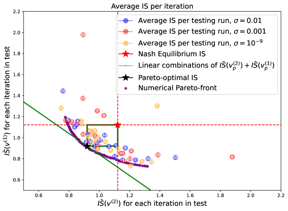
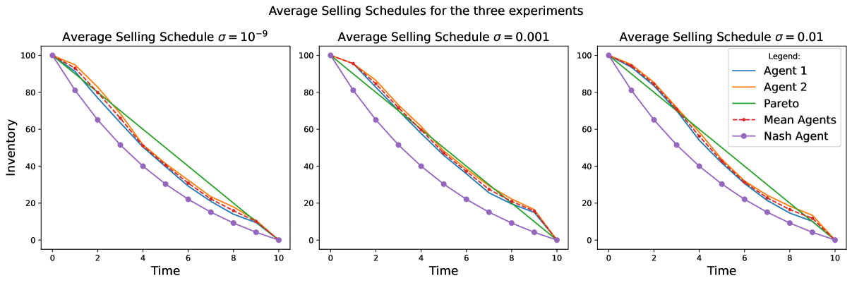
Figure 8 shows that, irrespective of the values considered for the volatility level $\sigma$ , the average strategy does not differ much from the Pareto-optimum TWAP strategy. In the zero noise case, the average strategy of the two agents tends to be slightly more front loaded, but still lies between the Nash and the Pareto-optimum. As the $\sigma$ value increases, and thus in the moderate noise and large noise cases, we can see how both the agents tend to be less aggressive at the beginning of their execution in order to adopt a larger selling rate towards the end of their execution. This behaviour is stronger the higher the $\sigma$ , due to the increased uncertainty brought by the asset volatility in addition to the price movements triggered by the trading of both the agents.

4.5 Variable volatility and misspecified dynamics

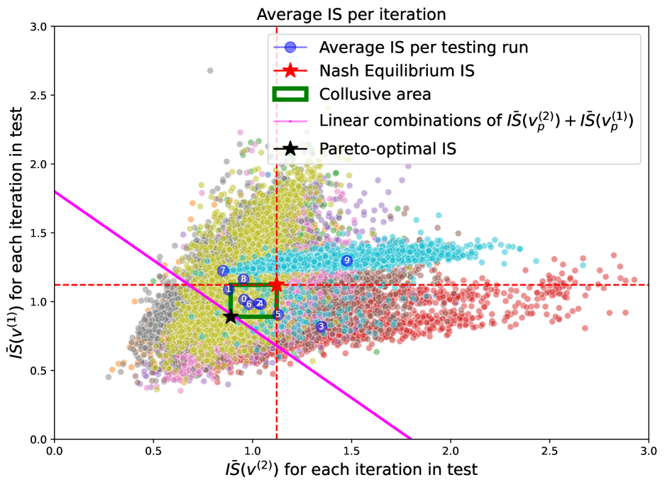
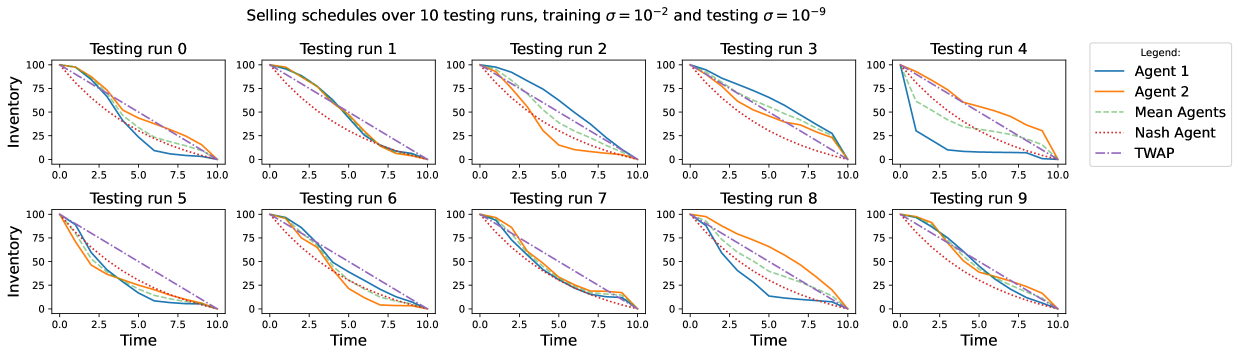
Our simulation results show that volatility plays an important role in determining the $IS$ in an iteration of the testing phase, although when averaging across the many iterations of a run, the results are more stable and consistent. In financial market, returns are known to be heteroscedastic, i.e. volatility varies with time. Thus, also from the practitioner’s point of view, it is interesting to study how agents, which are trained in an environment with a given level of volatility level, perform in a testing environment where the level of volatility is different. In particular, it is not a priori clear whether a collusive relationship between the two agents would still naturally arise when the price dynamics is different in the testing and in the training phase. Moreover, it is interesting to study how a change in the environment would impact the overall selling schedule and the corresponding costs. In the following, we study the agents’ behaviour in extreme cases, in order to better appreciate their behaviour under time-varying conditions. Specifically, using the same impact parameters as above in both phases, we learn the the weights of the DDQN algorithm in a training setting with $\sigma=10^{-9}$ and then we employ them in a testing environment where $\sigma=10^{-2}$ . We then repeat the experiment in the opposite case with the volatility parameters switched, i.e. training with $\sigma=10^{-2}$ and testing with $\sigma=10^{-9}$ .As before, we run $10$ testing runs of $2,500$ iterations each.

4.5.1 Training with zero noise and testing with large noise

When the agents are trained in an environment where $\sigma=10^{-9}$ and the weights of this training are used in a testing environment with $\sigma=10^{-2}$ , we find that the distribution of the $IS$ s per iteration is similar to the one that would be obtained in a both testing and training with $\sigma=10^{-2}$ scenario (see Figure 9). The centroids are still mostly distributed in the second, third and fourth quadrant, although some iterations and even a centroid, might end up in the first quadrant as in the $\sigma=10^{-9}$ case. In general, it can be seen how the centroids mostly lie in the collusive area of the graph, i.e in the square between the Pareto-optimal $IS$ and the Nash equilibrium, pointing out at the fact that collusive behaviours are still attainable even when the training dynamics are misspecified with respect to the testing ones.

Looking at Figure 10, we notice that the selling schedules are mostly intertwined, i.e. rarely the agents trade at the same rate. Traders can still be slow or fast depending on the rate adopted by the other agent. Comparing Figure 10 with Figure 9 we see that, as in the correctly specified case, the agent that trades faster gets the lower cost, while the slow trader achieves a larger $IS$ .

4.5.2 Training with large noise and testing with zero noise

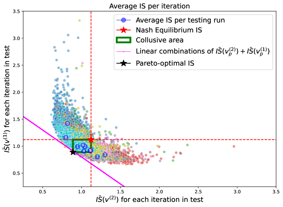
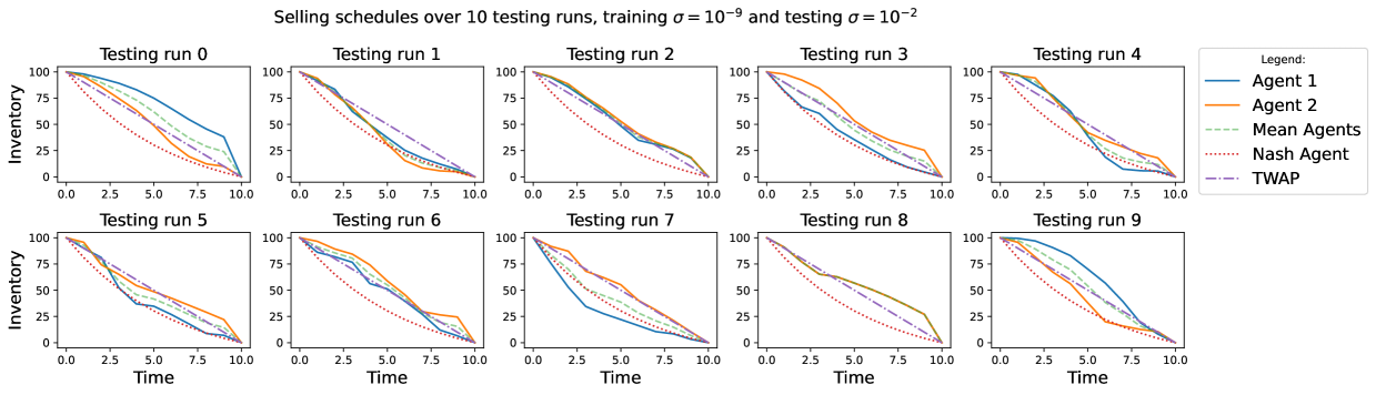
Figure 11 shows the result of the experiment where agents are trained in an environment where $\sigma=10^{-2}$ and tested in a market with $\sigma=10^{-9}$ . We observe that the $IS$ s are distributed in a way similar to the case where the agents were both tested and trained in an environment with $\sigma=10^{-9}$ . Still, the centroids lie in all but the first quadrant, and the majority of them lies in the collusive area, showing how even with misspecified dynamics, a collusive behaviour naturally arises in this game. The trading schedules adopted show the same kind of fast-slow trading behaviour between the agents, where still the slower trader has to pay higher costs in terms of $IS$ (see Figure 12).

Finally, irrespective of the encountered levels of volatility, it seems that what is more important is the market environment experienced during the training phase, thus the selling schedule implemented in a high volatility scenario with DDQN weights coming from a low volatility scenario are remarkably similar to the one found with both training and testing with $\sigma=10^{-9}$ , and vice versa when $\sigma=10^{-2}$ is used in training and the low volatility is encountered in the test. It might be concluded that once that the agents learn how to adopt a collusive behaviour in one volatility regime, they are able to still adopt a collusive behaviour when dealing with another volatility regime.

5 Conclusions

In this paper we have studied how collusive strategies arise in an open loop two players’ optimal execution game. We first have introduced the concept of collusive Pareto optima, that is, a vector of selling strategies whose IS is not dominated by the IS of other strategies for each iteration of the game. We furthermore showed how a Pareto-efficient set of solutions for this game exists and can be obtained as a solution to a multi-objective minimisation problem. Finally, we have shown how the Pareto-optimal strategy, that is indeed the collusion strategy in this setup, is the TWAP for risk-neutral agents.

As our main contribution, we have developed a Double Deep Q-Learning algorithm where two agents are trained using RL. The agents were trained and tested over several different scenarios where they learn how to optimally liquidate a position in the presence of the other agent and then, in the testing phase, they deploy their strategy leveraging on what learnt in the previous phase. The different scenarios, large, moderate and low volatility, helped us to shed light on how the trading interactions on the same asset made by two different agents, who are not aware of the other competitor, give rise to collusive strategies, i.e. strategies with a cost lower than a Nash equilibrium but higher than a proper collusion. This, in turn, is due to agents who keep trading at a different speed, thus adjusting the speed of their trading based on what the other agent is doing. Agents do not interact directly and are not aware of the other agent’s trading activity, thus strategies are learnt from the information coming from the impact on the asset price in a model-agnostic fashion.

Finally, we have studied how the agents interact when the volatility parameter in the training part is misspecified with respect to the one observed by the agents in the testing part. It turns out that the existence of collusive strategies are still arising, and thus robust with respect to settings when models parameters are time varying.

There are several possible extensions of our work. One obvious extension is to the setting where more than two agents are present and/or where more assets are liquidated, leading to a multi-asset and multi-agent market impact games, leveraging on the work done in [39]. Second, impact parameters are constant, while the problem becomes more interesting when liquidity is time-varying (see [29] for RL optimal execution with one agent). Third, we have considered a linear impact model, whereas it is known that impact coefficients are usually non-linear and might follow non-trivial intraday dynamics. Finally, the Almgren-Chriss model postulates a permanent and fixed impact, while many empirical results point toward its transient nature (see [6]). Interestingly, in this setting the Nash equilibrium of the market impact game shows price instabilities in some regime of parameters (see [20]), which are similar to market manipulations. It could be interesting to study if different market manipulation practices might arise when agents are trained, as in this paper, with RL techniques. The answer would be certainly of great interest also to regulators and supervising authorities.

Acknowledgements

The authors thank Sebastian Jaimungal for the useful discussions and insights. AM thanks Felipe Antunes for the useful discussions and insights. FL acknowledges support from the grant PRIN2022 DD N. 104 of February 2, 2022 ”Liquidity and systemic risks in centralized and decentralized markets”, codice proposta 20227TCX5W - CUP J53D23004130006 funded by the European Union NextGenerationEU through the Piano Nazionale di Ripresa e Resilienza (PNRR).

References

[1] Robert Kissell “Algorithmic trading methods: Applications using advanced statistics, optimization, and machine learning techniques” Academic Press, 2020
[2] Robert Almgren and Neill Chriss “Optimal execution of portfolio transactions” In Journal of Risk 3, 2000, pp. 5–39
[3] Alexander Schied and Tao Zhang “A State-Constrained Differential Game Arising in Optimal Portfolio Liquidation” In Mathematical Finance 27.3 Wiley Online Library, 2017, pp. 779–802
[4] Dimitri Bertsimas and Andrew W. Lo “Optimal control of execution costs” In Journal of Financial Markets 1.1 Elsevier, 1998, pp. 1–50
[5] Jean-Philippe Bouchaud, Yuval Gefen, Marc Potters and Matthieu Wyart “Fluctuations and response in financial markets: the subtle nature ofrandom’price changes” In Quantitative finance 4.2 IOP Publishing, 2003, pp. 176
[6] Jean-Philippe Bouchaud, J Doyne Farmer and Fabrizio Lillo “How markets slowly digest changes in supply and demand” In Handbook of financial markets: dynamics and evolution Elsevier, 2009, pp. 57–160
[7] Gueant, Olivier, Lehalle, Charles-Albert and Fernandez-Tapia, Joaquin “Optimal portfolio liquidation with limit orders” In SIAM Journal on Financial Mathematics 3.1 SIAM, 2012, pp. 740–764
[8] Jim Gatheral, Alexander Schied and Alla Slynko “Transient linear price impact and Fredholm integral equations” In Mathematical Finance: An International Journal of Mathematics, Statistics and Financial Economics 22.3 Wiley Online Library, 2012, pp. 445–474
[9] Anna A Obizhaeva and Jiang Wang “Optimal trading strategy and supply/demand dynamics” In Journal of Financial markets 16.1 Elsevier, 2013, pp. 1–32
[10] Olivier Guéant and Charles-Albert Lehalle “General intensity shapes in optimal liquidation” In Mathematical Finance 25.3 Wiley Online Library, 2015, pp. 457–495
[11] Alvaro Cartea, Sebastian Jaimungal and Josè Penalva “Algorithmic and high-frequency trading” Cambridge University Press, 2015
[12] Alvaro Cartea and Sebastian Jaimungal “Incorporating order-flow into optimal execution” In Mathematics and Financial Economics 10 Springer, 2016, pp. 339–364
[13] Philippe Casgrain and Sebastian Jaimungal “Trading algorithms with learning in latent alpha models” In Mathematical Finance 29.3 Wiley Online Library, 2019, pp. 735–772
[14] Frédéric Bucci et al. “Co-impact: Crowding effects in institutional trading activity” In Quantitative Finance 20.2 Taylor & Francis, 2020, pp. 193–205
[15] René Carmona and Joseph Yang “Predatory trading: a game on volatility and liquidity” In Preprint. URL: http://www. princeton. edu/rcarmona/download/fe/PredatoryTradingGameQF. pdf Citeseer, 2011
[16] Alessandro Micheli, Johannes Muhle-Karbe and Eyal Neuman “Closed-loop Nash competition for liquidity” In Mathematical Finance 33.4 Wiley Online Library, 2023, pp. 1082–1118
[17] Markus K Brunnermeier and Lasse Heje Pedersen “Predatory trading” In The Journal of Finance 60.4 Wiley Online Library, 2005, pp. 1825–1863
[18] Bruce Ian Carlin, Miguel Sousa Lobo and S Viswanathan “Episodic liquidity crises: Cooperative and predatory trading” In The Journal of Finance 62.5 Wiley Online Library, 2007, pp. 2235–2274
[19] Torsten Schöneborn and Alexander Schied “Liquidation in the face of adversity: stealth vs. sunshine trading” In EFA 2008 Athens Meetings Paper, 2009
[20] Alexander Schied and Tao Zhang “A market impact game under transient price impact” In Mathematics of Operations Research 44.1 INFORMS, 2019, pp. 102–121
[21] Samuel Drapeau, Peng Luo, Alexander Schied and Dewen Xiong “An FBSDE approach to market impact games with stochastic parameters” In arXiv preprint arXiv:2001.00622, 2019
[22] Eyal Neuman and Moritz Voß “Trading with the crowd” In Mathematical Finance 33.3 Wiley Online Library, 2023, pp. 548–617
[23] Rama Cont, Xin Guo and Renyuan Xu “Interbank lending with benchmark rates: Pareto optima for a class of singular control games” In Mathematical Finance 31.4 Wiley Online Library, 2021, pp. 1357–1393
[24] Rama Cont and Wei Xiong “Dynamics of market making algorithms in dealer markets: Learning and tacit collusion” In Mathematical Finance Wiley Online Library, 2022
[25] Shuo Sun, Rundong Wang and Bo An “Reinforcement learning for quantitative trading” In ACM Transactions on Intelligent Systems and Technology 14.3 ACM New York, NY, 2023, pp. 1–29
[26] Ben Hambly, Renyuan Xu and Huining Yang “Recent advances in reinforcement learning in finance” In Mathematical Finance 33.3 Wiley Online Library, 2023, pp. 437–503
[27] Brian Ning, Franco Ho Ting Lin and Sebastian Jaimungal “Double deep q-learning for optimal execution” In Applied Mathematical Finance 28.4 Taylor & Francis, 2021, pp. 361–380
[28] Matthias Schnaubelt “Deep reinforcement learning for the optimal placement of cryptocurrency limit orders” In European Journal of Operational Research 296.3 Elsevier, 2022, pp. 993–1006
[29] Andrea Macr‘ı and Fabrizio Lillo “Reinforcement Learning for Optimal Execution when Liquidity is Time-Varying” In arXiv e-prints: 2402.12049, 2024
[30] Michaël Karpe, Jin Fang, Zhongyao Ma and Chen Wang “Multi-agent reinforcement learning in a realistic limit order book market simulation” In Proceedings of the First ACM International Conference on AI in Finance, 2020, pp. 1–7
[31] Wenhang Bao and Xiao-yang Liu “Multi-agent deep reinforcement learning for liquidation strategy analysis” In arXiv preprint arXiv:1906.11046, 2019
[32] Ludo Waltman and Uzay Kaymak “Q-learning agents in a Cournot oligopoly model” In Journal of Economic Dynamics and Control 32.10 Elsevier, 2008, pp. 3275–3293
[33] Ibrahim Abada and Xavier Lambin “Artificial intelligence: Can seemingly collusive outcomes be avoided?” In Management Science 69.9 INFORMS, 2023, pp. 5042–5065
[34] Matthias Hettich “Algorithmic collusion: Insights from deep learning” In Available at SSRN 3785966, 2021
[35] Wei Xiong and Rama Cont “Interactions of market making algorithms” In Association for Computing Machinery, 2022
[36] Alvaro Cartea, Patrick Chang and Josè Penalva “Algorithmic collusion in electronic markets: The impact of tick size” In Available at SSRN 4105954, 2022
[37] Massimiliano Gobbi, F Levi, Gianpiero Mastinu and Giorgio Previati “On the analytical derivation of the Pareto-optimal set with applications to structural design” In Structural and Multidisciplinary Optimization 51 Springer, 2015, pp. 645–657
[38] Julian Blank and Kalyanmoy Deb “pymoo: Multi-Objective Optimization in Python” In IEEE Access 8, 2020, pp. 89497–89509
[39] Francesco Cordoni and Fabrizio Lillo “Instabilities in multi-asset and multi-agent market impact games” In Annals of Operations Research 336.1 Springer, 2024, pp. 505–539