DFAC Framework: Factorizing the Value Function via
Quantile Mixture for Multi-Agent Distributional Q-Learning

In this work, we consider a fully cooperative MARL environment modeled as a decentralized and partially observable Markov Decision Process (Dec-POMDP) (Oliehoek & Amato, 2016) with stocastic rewards, which is described as a tuple $\langle\mathbb{S}{},\mathbb{K}{},\mathbb{O}_{\mathrm{jt}},\mathbb{U}_{\mathrm{jt}},P{},O{},R{},\gamma{}\rangle$ and is defined as follows:

• •

  $\mathbb{S}{}$ is the finite set of global states in the environment, where $s{}^{\prime}\in\mathbb{S}{}$ denotes the next state of the current state $s{}\in\mathbb{S}{}$. The state information is optionally available during training, but not available to the agents during execution.

• •

  $\mathbb{K}{}=\{1,...,\mathrm{K}{}\}$ is the set of $\mathrm{K}{}$ agents. We use $k{}\in\mathbb{K}{}$ to denote the index of the agent.

• •

  $\mathbb{O}_{\mathrm{jt}}=\Pi_{k{}\in\mathbb{K}{}}\mathbb{O}{}_{k{}}$ is the set of joint observations. At each timestep, a joint observation $\mathbf{o}{}=\langle o{}_{1},...o{}_{\mathrm{K}}{}\rangle\in\mathbb{O}_{\mathrm{jt}}$ is received. Each agent $k{}$ is only able to observe its individual observation $o{}_{k{}}\in\mathbb{O}{}_{k{}}$.

• •

  $\mathbb{H}_{\mathrm{jt}}=\Pi_{k{}\in\mathbb{K}{}}\mathbb{H}{}_{k{}}$ is the set of joint action-observation histories. The joint history $\mathbf{h}{}=\langle h{}_{1},...h{}_{\mathrm{K}}{}\rangle\in\mathbb{H}_{\mathrm{jt}}$ concatenates all received observations and performed actions before a certain timestep, where $h{}_{k{}}\in\mathbb{H}{}_{k{}}$ represents the action-observation history from agent $k{}$.

• •

  $\mathbb{U}_{\mathrm{jt}}=\Pi_{k{}\in\mathbb{K}{}}\mathbb{U}{}_{k{}}$ is the set of joint actions. At each timestep, the entire group of the agents take a joint action $\mathbf{u}{}$, where $\mathbf{u}{}=\langle u{}_{1},...,u{}_{\mathrm{K}{}}\rangle\in\mathbb{U}_{\mathrm{jt}}$. The individual action $u{}_{k{}}\in\mathbb{U}_{k{}}$ of each agent $k{}$ is determined based on its stochastic policy $\pi{}_{k{}}(u{}_{k{}}|h{}_{k{}}):\mathbb{H}{}_{k{}}\times\mathbb{U}{}_{k{}}\rightarrow[0,1]$, expressed as $u{}_{k{}}\sim\pi{}_{k{}}(\cdot|h{}_{k{}})$. Similarly, in single agent scenarios, we use $u$ and $u^{\prime}$ to denote the actions of the agent at state $s$ and $s^{\prime}$ under policy $\pi$, respectively.

• •

  $\mathbb{T}{}=\{1,...,\mathrm{T}{}\}$ represents the set of timesteps with horizon $\mathrm{T}{}$, where the index of the current timestep is denoted as $t{}\in\mathbb{T}{}$. $s^{t}$, $o^{t}$, $h^{t}$, and $u^{t}$ correspond to the environment information at timestep $t$.

• •

  The transition function $P{}(s{}^{\prime}|s{},\mathbf{u}{}):\mathbb{S}{}\times\mathbb{U}_{\mathrm{jt}}\times\mathbb{S}{}\rightarrow[0,1]$ specifies the state transition probabilities. Given $s$ and $\mathbf{u}$, the next state is denoted as $s{}^{\prime}\sim P{}(\cdot|s{},\mathbf{u}{})$.

• •

  The observation function $O{}({\mathbf{o}{}}|s{}):\mathbb{O}_{\mathrm{jt}}\times\mathbb{S}{}\rightarrow[0,1]$ specifies the joint observation probabilities. Given $s{}$, the joint observation is represented as $\mathbf{o}{}\sim O{}(\cdot|s{})$.

• •

  $R{}(r|s{},\mathbf{u}{}):\mathbb{S}{}\times\mathbb{U}_{\mathrm{jt}}\times\mathbb{R}\rightarrow[0,1]$ is the joint reward function shared among all agents. Given $s$, the team reward is expressed as $r\sim R{}(\cdot|s{},\mathbf{u}{})$.

• •

  $\gamma{}\in\mathbb{R}$ is the discount factor with value within $(0,1]$.

Under such an MARL formulation, this work concentrates on CTDE value function factorization methods, where the agents are trained in a centralized fashion and executed in a decentralized manner. In other words, the joint observation history $\mathbf{h}{}$ is available during the learning processes of individual policies $[\pi{}_{k{}}]_{k{}\in\mathbb{K}{}}$. During execution, each agent’s policy $\pi{}_{k{}}$ only conditions on its observation history $h{}_{k{}}$.

IGM is necessary for value function factorization (Son et al., 2019). For a joint action-value function $Q{}_{\mathrm{jt}{}}(\mathbf{h}{},\mathbf{u}{}):\mathbb{H}_{\mathrm{jt}}\times\mathbb{U}_{\mathrm{jt}}\rightarrow\mathbb{R}$, if there exist $\mathrm{K}{}$ individual utility functions $[Q{}_{k}{}(h{}_{k}{},u{}_{k}{}):\mathbb{H}{}_{k{}}\times\mathbb{U}{}_{k{}}\rightarrow\mathbb{R}]_{k{}\in\mathbb{K}{}}$ such that the following condition holds:

then $[Q{}_{k}{}]_{k{}\in\mathbb{K}{}}$ are said to satisfy IGM for $Q{}_{\mathrm{jt}{}}$ under $\mathbf{h}{}$. In this case, we also say that $Q{}_{\mathrm{jt}{}}(\mathbf{h}{},\mathbf{u}{})$ is factorized by $[Q{}_{k}{}(h{}_{k}{},u{}_{k}{})]_{k{}\in\mathbb{K}{}}$ (Son et al., 2019). If $Q{}_{\mathrm{jt}{}}$ in a given task is factorizable under all $\mathbf{h}{}\in\mathbb{H}_{\mathrm{jt}}$, we say that the task is factorizable. Intuitively, factorizable tasks indicate that there exists a factorization such that each agent can select the greedy action according to their individual utilities $[Q{}_{k}{}]_{k{}\in\mathbb{K}{}}$ independently in a decentralized fashion. This enables the optimal individual actions to implicitly achieve the optimal joint action across the $\mathrm{K}{}$ agents. Since there is no individual reward, the factorized utilities do not estimate expected returns on their own (Guestrin et al., 2001) and are different from the value function definition commonly used in SARL.

Based on IGM, value function factorization methods enable centralized training for factorizable tasks, while maintaining the ability for decentralized execution. In this work, we consider two such methods, VDN and QMIX, which can solve a subset of factorizable tasks that satisfies Additivity (Eq. (2)) and Monotonicity (Eq. (3)), respectively, given by:

where $M$ is a monotonic function that satisfies $\frac{\partial M}{\partial Q{}_{k}{}}\geq 0,\forall k{}\in\mathbb{K}{}$, and conditions on the state $s$ if the information is available during training. Either of these two equation is a sufficient condition for IGM (Son et al., 2019).

For notational simplicity, we consider a degenerated case with only a single agent, and the environment is fully observable until the end of Section 2.6. Distributional RL generalizes classic expected RL methods by capturing the full return distribution $Z{}(s{},u{})$ instead of the expected return $Q{}(s{},u{})$, and outperforms expected RL methods in various single-agent RL domains (Bellemare et al., 2017, 2019; Dabney et al., 2018b, a; Rowland et al., 2019; Yang et al., 2019). Moreover, distributional RL enables improvements (Nikolov et al., 2019; Zhang & Yao, 2019; Mavrin et al., 2019) that require the information of the full return distribution. We define the distributional Bellman operator $\mathcal{T}^{\pi}$ as follows:

and the distributional Bellman optimality operator $\mathcal{T}^{*}$ as:

where $u{}^{\prime*}=\arg\max_{u^{\prime}}\mathbb{E}[Z{}(s{}^{\prime},u^{\prime})]$ is the optimal action at state $s{}^{\prime}$, and the expression $X\stackrel{{\scriptstyle D}}{{=}}Y$ denotes that random variable $X$ and $Y$ follow the same distribution. Given some initial distribution $Z_{0}$, $Z{}$ converges to the return distribution $Z{}^{\pi}$ under $\pi$, contracting in terms of $p$-Wasserstein distance for all $p\in[1,\infty)$ by applying $\mathcal{T}^{\pi}$ repeatedly; while $Z{}$ alternates between the optimal return distributions in the set $\mathcal{Z{}}^{*}:=\{Z^{\pi^{*}}:\pi^{*}\in\Pi^{*}\}$, under the set of optimal policies $\Pi^{*}$ by repeatedly applying $\mathcal{T}^{*}$ (Bellemare et al., 2017). The $p$-Wasserstein distance $W_{p}$ between the probability distributions of random variables $X$, $Y$ is given by:

where $(F^{-1}_{X},F^{-1}_{Y})$ are quantile functions of $(X,Y)$.

The relationship between the cumulative distribution function (CDF) $F_{X}$ and the quantile function $F^{-1}_{X}$ (the generalized inverse CDF) of random variable $X$ is formulated as:

The expectation of $X$ expressed in terms of $F^{-1}_{X}(\omega{})$ is:

In (Dabney et al., 2018b), the authors model the value function as a quantile function $F^{-1}{}(s{},u{}|\omega{})$. During optimization, a pair-wise sampled temporal difference (TD) error $\delta$ for two quantile samples $\omega{},\omega{}^{\prime}\sim U([0,1])$ is defined as:

The pair-wise loss $\rho{}^{\kappa}_{\omega{}}$ is then defined based on the Huber quantile regression loss $\mathcal{L}_{\kappa}{}$ (Dabney et al., 2018b) with threshold $\kappa=1$, and is formulated as follows:

Given $\mathrm{N}{}$ quantile samples $[\omega{}_{i}]^{\mathrm{N}}_{i=1}$ to be optimized with regard to $\mathrm{N}^{\prime}$ target quantile samples $[\omega{}_{j}]^{\mathrm{N}^{\prime}}_{j=1}$, the total loss $\mathcal{L}{}(s{},u{},r{},s{}^{\prime})$ is defined as the sum of the pair-wise losses, and is expressed as the following:

Implicit quantile network (IQN) (Dabney et al., 2018a) is relatively light-weight when it is compared to other distributional RL methods. It approximates the return distribution $Z{}(s{},u{})$ by an implicit quantile function $F^{-1}{}(s{},u{}|\omega{})=g{}(\psi{}(s{}),\phi{}(\omega{}))_{u}{}$ for some differentiable functions $g{}$, $\psi$, and $\phi$. Such an architecture is a type of universal value function approximator (UVFA) (Schaul et al., 2015), which generalizes its predictions across states $s{}\in\mathbb{S}{}$ and goals $\omega{}\in[0,1]$, with the goals defined as different quantiles of the return distribution. In practice, $\phi{}$ first expands the scalar $\omega$ to an $n$-dimensional vector by $[\cos(\pi i\omega)]^{\mathrm{n}{}-1}_{i=0}$, followed by a single hidden layer with weights $[w_{ij}]$ and biases $[b_{j}]$ to produce a quantile embedding $\phi{}(\omega{})=[\phi(\omega{})_{j}]^{\text{dim}(\phi{}(\omega{}))-1}_{j=0}$. The expression of $\phi(\omega{})_{j}$ can be represented as the following:

where $\mathrm{n}{}=64$ and $\text{dim}(\phi(\omega{}))=\text{dim}(\psi(s{}))$. Then, $\phi{}(\omega{})$ is combined with the state embedding $\psi{}(s{})$ by the element-wise (Hadamard) product ($\odot$), expressed as $g:=\psi{}\odot\phi{}$. The loss of IQN is defined as Eq. (12) by sampling a batch of $\mathrm{N}{}$ and $\mathrm{N}^{\prime}{}$ quantiles from the policy network and the target network respectively. During execution, the action with the largest expected return $Q{}(s{},u{})$ is chosen. Since IQN does not model the expected return explicitly, $Q{}(s{},u{})$ is approximated by calculating the mean of the sampled return through $\hat{\mathrm{N}}{}$ quantile samples $\hat{\omega}{}_{i}\sim U([0,1]),\forall i\in[1,\hat{\mathrm{N}}{}]$ based on Eq. (8), expressed as follows:

Multiple quantile functions (e.g., IQNs) sharing the same quantile $\omega{}$ may be combined into a single quantile function $F^{-1}{}(\omega{})$, in a form of quantile mixture expressed as follows:

where $[F^{-1}_{k{}}(\omega{})]_{k{}\in\mathbb{K}{}}$ are quantile functions, and $[\beta{}_{k{}}]_{k{}\in\mathbb{K}{}}$ are model parameters (Karvanen, 2006). The condition for $[\beta{}_{k{}}]_{k{}\in\mathbb{K}{}}$ is that $F^{-1}{}(\omega{})$ must satisfy the properties of a quantile function. The concept of quantile mixture is analogous to the mixture of multiple probability density functions (PDFs), expressed as follows:

where $[f{}_{k{}}(x)]_{k{}\in\mathbb{K}{}}$ are PDFs, $\sum^{\mathrm{K}{}}_{k{}=1}\alpha{}_{k{}}=1$, and $\alpha{}_{k{}}\geq 0$.

Since IGM is necessary for value function factorization, a distributional factorization that satisfies IGM is required for factorizing stochastic value functions. We first discuss a naive distributional factorization that simply replaces deterministic utilities $Q$ with stochastic utilities $Z$. Then, we provide a theorem to show that the naive distributional factorization is insufficient to guarantee the IGM condition.

In order to satisfy DIGM for stochastic utilities, an alternative factorization strategy is necessary.

We propose Mean-Shape Decomposition and the DFAC framework to ensure that DIGM is satisfied for stochastic utilities.

We propose DFAC to decompose a joint return distribution $Z{}_{\mathrm{jt}{}}$ into its deterministic part $Z{}_{\text{mean}}$ (i.e., expected value) and stochastic part $Z{}_{\text{shape}}$ (i.e., higher moments), which are approximated by two different functions $\Psi$ and $\Phi$, respectively. The factorization function $\Psi$ is required to precisely factorize the expectation of $Z{}_{\mathrm{jt}{}}$ in order to satisfy DIGM. On the other hand, the shape function $\Phi$ is allowed to roughly factorize the shape of $Z{}_{\mathrm{jt}{}}$, since the main objective of modeling the return distribution is to assist non-linear approximation of the expectation of $Z{}_{\mathrm{jt}{}}$ (Lyle et al., 2019), rather than accurately model the shape of $Z{}_{\mathrm{jt}{}}$.

Theorem. 2 reveals that the choice of $\Psi$ determines whether IGM holds, regardless of the choice of $\Phi$, as long as $\mathbb{E}[\Phi]=0$. Under this setting, any differentiable factorization function of deterministic variables can be extended to a factorization function of random variables. Such a decomposition enables approximation of joint distributions for all factorizable tasks under appropriate choices of $\Psi{}$ and $\Phi{}$.

In this section, we provide a practical implementation of the shape function $\Phi$ in DFAC, effectively extending any differentiable factorization function $\Psi{}$ (e.g., the additive function of VDN, the monotonic mixing network of QMIX, etc.) that satisfies the IGM condition into its DFAC variant.

Theoretically, the sum of random variables appeared in DDN and DMIX can be described precisely by a joint CDF. However, the exact derivation of this joint CDF is usually computationally expensive and impractical (Lin et al., 2019). As a result, DFAC utilizes the property of quantile mixture to approximate the shape function $\Phi{}$ in $\mathrm{O}(\mathrm{K}\mathrm{N})$ time.

Based on Theorem 3, the quantile function $F^{-1}_{\mathrm{shape}}$ of $Z_{\mathrm{shape}}$ in DFAC can be approximated by the following:

where $F^{-1}_{\text{state}}(s{}|\omega{})$ and $[\beta{}_{k}(s)]_{k{}\in\mathbb{K}{}}$ are respectively generated by function approximators $\Lambda_{\text{state}}(s{}|\omega{})$ and $[\Lambda_{k}(s{})]_{k{}\in\mathbb{K}{}}$, satisfying constraints $\beta{}_{k}(s)\geq 0,\forall k{\in\mathbb{K}{}}$ and $\int_{0}^{1}F^{-1}_{\text{state}}(s|\omega{})\ \mathrm{d}\omega=0$. The term $F^{-1}_{\text{state}}$ models the shape of an additional state-dependent utility (introduced by QMIX at the last layer of the mixing network), which extends the state-dependent bias in QMIX to a full distribution. The full network architecture of DFAC is illustrated in Fig. 1.

This transformation enables DFAC to decompose the quantile representation of a joint distribution into the quantile representations of individual utilities. In this work, $\Phi{}$ is implemented by a large IQN composed of multiple IQNs, optimized through the loss function defined in Eq. (12).

In order to validate the proposed DFAC framework, we next discuss the DFAC variants of two representative factorization methods: VDN and QMIX. DDN extends VDN to its DFAC variant, expressed as:

$Z_{\mathrm{mean}}=\sum_{k\in\mathbb{K}{}}Q_{k}$, $Z_{\mathrm{shape}}=\sum_{k\in\mathbb{K}{}}(Z_{k}-Q_{k})$; while DMIX extends QMIX to its DFAC variant, expressed as:

$Z_{\mathrm{mean}}=M{}(Q_{1},...,Q_{\mathrm{K}}|s)$, $Z_{\mathrm{shape}}=\sum_{k\in\mathbb{K}{}}(Z_{k}-Q_{k})$.

Both DDN and DMIX choose $F^{-1}_{\text{state}}=0$ and $[\beta{}_{k}=1]_{k{}\in\mathbb{K}{}}$ for simplicity. Automatically learning the values of $F^{-1}_{\text{state}}$ and $[\beta{}_{k}]_{k{}\in\mathbb{K}{}}$ is proposed as future work.

Environment. We verify the DFAC framework in the SMAC benchmark environments (Samvelyan et al., 2019) built on the popular real-time strategy game StarCraft II. Instead of playing the full game, SMAC is developed for evaluating the effectiveness of MARL micro-management algorithms. Each environment in SMAC contains two teams. One team is controlled by a decentralized MARL algorithm, with the policies of the agents conditioned on their local observation histories. The other team consists of enemy units controlled by the built-in game artificial intelligence based on carefully handcrafted heuristics, which is set to its highest difficulty equal to seven. The overall objective is to maximize the win rate for each battle scenario, where the rewards employed in our experiments follow the default settings of SMAC. The default settings use shaped rewards based on the damage dealt, enemy units killed, and whether the RL agents win the battle. If there is no healing unit in the enemy team, the maximum return of an episode (i.e., the score) is $20$; otherwise, it may exceed $20$, since enemies may receive more damages after healing or being healed.

The environments in SMAC are categorized into three different levels of difficulties: Easy, Hard, and Super Hard scenarios (Samvelyan et al., 2019). In this paper, we focus on all Super Hard scenarios including (a) 6h_vs_8z, (b) 3s5z_vs_3s6z, (c) MMM2, (d) 27m_vs_30m, and (e) corridor, since these scenarios have not been properly addressed in the previous literature without the use of additional assumptions such as intrinsic reward signals (Du et al., 2019), explicit communication channels (Zhang et al., 2019; Wang et al., 2019), common knowledge shared among the agents (de Witt et al., 2019; Wang et al., 2020), and so on. Three of these scenarios have their maximum scores higher than $20$. In 3s5z_vs_3s6z, the enemy Stalkers have the ability to regenerate shields; in MMM2, the enemy Medivacs can heal other units; in corridor, the enemy Zerglings slowly regenerate their own health.

Hyperparameters. For all of our experimental results, the training length is set to 8M timesteps, where the agents are evaluated every 40k timesteps with 32 independent runs. The curves presented in this section are generated based on five different random seeds. The solid lines represent the median win rate, while the shaded areas correspond to the $25^{\text{th}}$ to $75^{\text{th}}$ percentiles. For a better visualization, the presented curves are smoothed by a moving average filter with its window size set to 11. The detailed hyperparameter setups are provided in the supplementary material.

Baselines. We select IQL, VDN, and QMIX as our baseline methods, and compare them with their distributional variants in our experiments. The configurations are optimized so as to provide the best performance for each of the methods considered. Since we tuned the hyperparameters of the baselines, their performances are better than those reported in (Samvelyan et al., 2019). The hyperparameter searching process is detailed in the supplementary material.

In order to validate our assumption that distributional RL is beneficial to the MARL domain, we first employ the simplest training algorithm, IQL, and extend it to its distributional variant, called DIQL. DIQL is simply a modified IQL that uses IQN as its underlying RL algorithm without any additional modification or enhancements (Matignon et al., 2007; Lyu & Amato, 2020).

From Figs. 3(a)-3(e) and Tables 4-4, it is observed that DIQL is superior to IQL even without utilizing any value function factorization methods. This validates that distributional RL has beneficial influences on MARL, when it is compared to RL approaches based only on expected values.

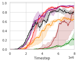
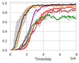
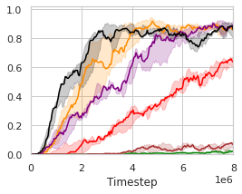
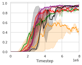
In order to inspect the effectiveness and impacts of DFAC on learning curves, win rates, and scores, we next summarize the results of the baselines as well as their DFAC variants on the Super Hard scenarios in Fig. 3(a)-(e) and Table 4-4.

Fig. 3(a)-(e) plot the learning curves of the baselines and their DFAC variants, with the final win rates presented in Table 4, and their final scores reported in Table 4. The win rates indicate how often do the player’s team wins, while the scores represent how well do the player’s team performs. Despite the fact that SMAC’s objective is to maximize the win rate, the true optimization goal of MARL algorithms is the averaged score. In fact, these two metrics are not always positively correlated (e.g., VDN and QMIX in 6h_vs_8z and 3s5z_vs_3s6z, and QMIX and DMIX in 3s5z_vs_3s6z).

It can be observed that the learning curves of DDN and DMIX grow faster and achieve higher final win rates than their corresponding baselines. In the most difficult map: 6h_vs_8z, most of the methods fail to learn an effective policy except for DDN and DMIX. The evaluation results also show that DDN and DMIX are capable of performing consistently well across all Super Hard maps with high win rates. In addition to the win rates, Table 4 further presents the final averaged scores achieved by each method, and provides deeper insights into the advantages of the DFAC framework by quantifying the performances of the learned policies of different methods.

The improvements in win rates and scores are due to the benefits offered by distributional RL (Lyle et al., 2019), which enables the distributional variants to work more effectively in MARL environments. Moreover, the evaluation results reveal that DDN performs especially well in most environments despite its simplicity. Further validations of DDN and DMIX on our self-designed Ultra Hard scenarios that are more difficult than Super Hard scenarios can be found in our GitHub repository (https://github.com/j3soon/dfac), along with the gameplay recording videos.

References

- Bellemare et al. (2017) Bellemare, M. G., Dabney, W., and Munos, R. A distributional perspective on reinforcement learning. In Proc. Int. Conf. on Machine Learning (ICML), pp. 449–458, Jul. 2017.
- Bellemare et al. (2019) Bellemare, M. G., Roux, N. L., Castro, P. S., and Moitra, S. Distributional reinforcement learning with linear function approximation. arXiv preprint arXiv:1902.03149, 2019.
- Dabney et al. (2018a) Dabney, W., Ostrovski, G., Silver, D., and Munos, R. Implicit quantile networks for distributional reinforcement learning. In Proc. Int. Conf. on Machine Learning (ICML), pp. 1096–1105, Jul. 2018a.
- Dabney et al. (2018b) Dabney, W., Rowland, M., Bellemare, M. G., and Munos, R. Distributional reinforcement learning with quantile regression. In Proc. AAAI Conf. on Artificial Intelligence (AAAI), pp. 2892–2901, Feb. 2018b.
- de Witt et al. (2019) de Witt, C. S., Foerster, J., Farquhar, G., Torr, P., Böhmer, W., and Whiteson, S. Multi-agent common knowledge reinforcement learning. In Advances in Neural Information Processing Systems, pp. 9924–9935, 2019.
- Du et al. (2019) Du, Y., Han, L., Fang, M., Liu, J., Dai, T., and Tao, D. Liir: Learning individual intrinsic reward in multi-agent reinforcement learning. In Advances in Neural Information Processing Systems, pp. 4405–4416, 2019.
- Guestrin et al. (2001) Guestrin, C., Koller, D., and Parr, R. Multiagent planning with factored mdps. In NIPS, 2001.
- Karvanen (2006) Karvanen, J. Estimation of quantile mixtures via l-moments and trimmed l-moments. Computational Statistics & Data Analysis, 51:947–959, 11 2006. doi: 10.1016/j.csda.2005.09.014.
- Lin et al. (2019) Lin, Z., Zhao, L., Yang, D., Qin, T., Liu, T.-Y., and Yang, G. Distributional reward decomposition for reinforcement learning. In Advances in Neural Information Processing Systems, pp. 6212–6221, 2019.
- Lyle et al. (2019) Lyle, C., Bellemare, M. G., and Castro, P. S. A comparative analysis of expected and distributional reinforcement learning. In Proc. AAAI Conf. on Artificial Intelligence (AAAI), pp. 4504–4511, Feb. 2019.
- Lyu & Amato (2020) Lyu, X. and Amato, C. Likelihood quantile networks for coordinating multi-agent reinforcement learning. In Proceedings of the 19th International Conference on Autonomous Agents and MultiAgent Systems, pp. 798–806, 2020.
- Matignon et al. (2007) Matignon, L., Laurent, G., and Fort-Piat, N. Hysteretic q-learning : an algorithm for decentralized reinforcement learning in cooperative multi-agent teams. pp. 64 – 69, 12 2007. doi: 10.1109/IROS.2007.4399095.
- Mavrin et al. (2019) Mavrin, B., Yao, H., Kong, L., Wu, K., and Yu, Y. Distributional reinforcement learning for efficient exploration. In Proc. Int. Conf. on Machine Learning (ICML), pp. 4424–4434, Jul. 2019.
- Nikolov et al. (2019) Nikolov, N., Kirschner, J., Berkenkamp, F., and Krause, A. Information-directed exploration for deep reinforcement learning. In Proc. Int. Conf. on Learning Representations (ICLR), May 2019. URL https://openreview.net/forum?id=Byx83s09Km.
- Oliehoek & Amato (2016) Oliehoek, F. A. and Amato, C. A Concise Introduction to Decentralized POMDPs. Springer, 2016. ISBN 3319289276.
- Oliehoek et al. (2016) Oliehoek, F. A., Amato, C., et al. A concise introduction to decentralized POMDPs, volume 1. Springer, 2016.
- Rashid et al. (2018) Rashid, T. et al. QMIX: Monotonic value function factorisation for deep multi-agent reinforcement learning. In Proc. Int. Conf. on Machine Learning (ICML), pp. 4295–4304, Jul. 2018.
- Rowland et al. (2019) Rowland, M. et al. Statistics and samples in distributional reinforcement learning. In Proc. Int. Conf. on Machine Learning (ICML), pp. 5528–5536, Jul. 2019.
- Samvelyan et al. (2019) Samvelyan, M. et al. The starcraft multi-agent challenge. In Proc. Int. Conf. on Autonomous Agents and MultiAgent Systems (AAMAS), pp. 2186–2188, May 2019.
- Schaul et al. (2015) Schaul, T., Horgan, D., Gregor, K., and Silver, D. Universal value function approximators. In International conference on machine learning, pp. 1312–1320, 2015.
- Son et al. (2019) Son, K., Kim, D., Kang, W. J., Hostallero, D. E., and Yi, Y. QTRAN: Learning to factorize with transformation for cooperative multi-agent reinforcement learning. In Proc. Int. Conf. on Machine Learning (ICML), pp. 5887–5896, Jul. 2019.
- Sunehag et al. (2018) Sunehag, P. et al. Value-decomposition networks for cooperative multi-agent learning based on team reward. In Proc. Int. Conf. on Autonomous Agents and MultiAgent Systems (AAMAS), pp. 2085–2087, May 2018.
- Tan (1993) Tan, M. Multi-agent reinforcement learning: Independent versus cooperative agents. In Proc. Int. Conf. on Machine Learning (ICML), pp. 330–337, Jun. 1993. ISBN 1558603077.
- Wang et al. (2019) Wang, T., Wang, J., Zheng, C., and Zhang, C. Learning nearly decomposable value functions via communication minimization. arXiv preprint arXiv:1910.05366, 2019.
- Wang et al. (2020) Wang, T., Dong, H., Lesser, V., and Zhang, C. Multi-agent reinforcement learning with emergent roles. arXiv preprint arXiv:2003.08039, 2020.
- Yang et al. (2019) Yang, D. et al. Fully parameterized quantile function for distributional reinforcement learning. In Proc. Conf. Advances in Neural Information Processing Systems (NeurIPS), pp. 6190–6199, Dec. 2019.
- Zhang & Yao (2019) Zhang, S. and Yao, H. Quota: The quantile option architecture for reinforcement learning. In Proc. AAAI Conf. on Artificial Intelligence (AAAI), pp. 5797–5804, Feb. 2019.
- Zhang et al. (2019) Zhang, S. Q., Zhang, Q., and Lin, J. Efficient communication in multi-agent reinforcement learning via variance based control. In Advances in Neural Information Processing Systems, pp. 3230–3239, 2019.
See pages - of supp.pdf