Diagrams realizing prescribed sublink diagrams for virtual links and welded links

Naoko Kamada Graduate School of Science, Nagoya City University
1 Yamanohata, Mizuho-cho, Mizuho-ku, Nagoya, Aichi 467-8501 Japan

Abstract.

Jin and Lee [3] proved the following: Suppose that $D_{1},\dots,D_{n}$ are link diagrams. Given a link $L$ which is partitioned into sublinks $L_{1},\dots,L_{n}$ admitting diagrams $D_{1},\dots,D_{n}$ respectively, there is a diagram $D$ of $L$ whose restrictions to $L_{1},\dots,L_{n}$ are isotopic to $D_{1},\dots,D_{n}$ , respectively. In this paper we show that a similar result does hold for welded links and does not for virtual links.

This work was supported by JSPS KAKENHI Grant Number 19K03496.

1. Introduction

G. T. Jin and J. H. Lee [3] proved the following theorem.

Theorem 1 (G. T. Jin and J. H. Lee [3]).

Suppose that $D_{1},\dots,D_{n}$ are link diagrams. Given a link $L$ which is partitioned into sublinks $L_{1},\dots,L_{n}$ admitting diagrams $D_{1},\dots,D_{n}$ respectively, there is a diagram $D$ of $L$ whose restrictions to $L_{1},\dots,L_{n}$ are isotopic in $\mathbb{R}^{2}$ to $D_{1},\dots,D_{n}$ , respectively.

Virtual links were introduced by L. H. Kauffman [8] as equivalence classes of virtual link diagrams in $\mathbb{R}^{2}$ under a certain equivalence relation. They are in one-to-one correspondence with stable equivalence classes of links in thickened surfaces [1, 7]. Welded links were introduced by R. Fenn R. Rimanyi, and C. Rouke [2] as equivalence classes of welded link diagrams in $\mathbb{R}^{2}$ under another equivalence relation. Both virtual links and welded links are generalizations of links.

In this paper we prove the following.

Theorem 2.

Suppose that $D_{1},\dots,D_{n}$ are diagrams of welded links. Given a welded link $L$ which is partitioned into sublinks $L_{1},\dots,L_{n}$ admitting diagrams $D_{1},\dots,D_{n}$ respectively, there is a diagram $D$ of $L$ whose restrictions to $L_{1},\dots,L_{n}$ are isotopic in $\mathbb{R}^{2}$ to $D_{1},\dots,D_{n}$ , respectively.

A similar statement to Theorems 1 and 2 does not hold for virtual links.

Theorem 3.

There exist diagrams $D_{1}$ and $D_{2}$ of virtual links, and a virtual link $L$ which is partitioned into $L_{1}$ and $L_{2}$ admitting diagrams $D_{1}$ and $D_{2}$ such that $L$ does not admit any diagram $D$ whose restrictions to $L_{1}$ and $L_{2}$ are isotopic in $\mathbb{R}^{2}$ to $D_{1}$ and $D_{2}$ , respectively.

2. Virtual links and welded links

We recall virtual links and welded links.

In this paper a diagram means a collection of immersed oriented loops in $\mathbb{R}^{2}$ such that the multiple points are transverse double points which are classified into classical crossings and virtual crossings: A classical crossing is a crossing with over/under information as usual in knot theory, and a virtual crossing is a crossing without over/under information [8]. A virtual crossing is depicted as a crossing encircled with a small circle. (Such a circle is not considered as a component of the diagram.) A classical crossing is also called a positive or negative crossing according to the sign of the crossing as usual in knot theory.

Two diagrams are v-equivalent or equivalent as virtual links if they are related by a finite sequence of local moves depicted in Figure 1 except WR up to isotopies of $\mathbb{R}^{2}$ . A virtual link is an equivalence class of diagrams under this equivalence relation.

Two diagrams are w-equivalent or equivalent as welded links if they are related by a finite sequence of local moves depicted in Figure 1 up to isotopies of $\mathbb{R}^{2}$ . A welded link is an equivalence class of diagrams under this equivalence relation.

A diagram without virtual crossings is called a classical link diagram. Two classical link diagrams are r-equivalent or equivalent as classical links if they are related by a finite sequence of local moves R1, R2 and R3 depicted in Figure 1 up to isotopies of $\mathbb{R}^{2}$ .

It is known that two classical link diagrams are equivalent as classical links if and only if they are equivalent as virtual (or welded) links. In this sense, virtual links and welded links are generalizations of classical links.

R1 R2 R3

VR1 VR2 VR3 VR4

Figure 1. Moves

Let $D^{\prime}$ be a diagram obtained from a diagram $D$ by one of the local moves depicted in Figure 1, a support of the move is a region $M$ in $\mathbb{R}^{2}$ which is homeomorphic to the $2$ -disk such that $D$ and $D^{\prime}$ are identical in $\mathbb{R}^{2}\setminus M$ and that $D\cap M$ and $D^{\prime}\cap D^{\prime}$ are depicted in the figure.

A detour move is a deformation of a diagram depicted in Figure 2 (i), where the box stands for a diagram which does not change. Two diagrams related by a detour move are equivalent as virtual links and as welded links.

An over detour move is a deformation of a virtual/welded link diagram in Figure 2 (ii). Two diagrams related by a detour move are equivalent as welded links.

Refer to caption — Figure 2. Two detour moves

3. Proof of Theorem 2

We introduce three moves depicted in Figure 3, which do not change the equivalence class of a diagram as a welded link.

For each move in the figure, in the left hand side of the move, let $\alpha$ be the vertical arc and let $v_{0},v_{1},\dots,v_{m}$ be crossings on $\alpha$ appearing in this order from the bottom to the top. Let $\beta_{0},\beta_{1},\dots,\beta_{m}$ be the arcs intersecting $\alpha$ at $v_{0},v_{1},\dots,v_{m}$ , respectively. Move $\beta$ toward the top along $\alpha$ and we obtain an arc $\beta_{0}^{\prime}$ as in the right hand side.

(i) An under finger move is as follows: At $v_{0}$ , $\beta_{0}$ is under $\alpha$ . For each $i\in\{1,\dots,m\}$ , when $v_{i}$ is a classical crossing, the two crossings of $\beta_{0}^{\prime}$ and $\beta_{i}$ are classical crossings where $\beta_{0}^{\prime}$ is under $\beta_{i}$ . When $v_{i}$ is a virtual crossing, the two crossings of $\beta_{0}^{\prime}$ and $\beta_{i}$ are virtual crossings. The intersection of $\beta_{0}^{\prime}$ and $\alpha$ is a classical crossing where $\beta_{0}^{\prime}$ is under $\alpha$ .

(ii) An over finger move is as follows: At $v_{0}$ , $\beta_{0}$ is over $\alpha$ . For each $i\in\{1,\dots,m\}$ , the two crossings of $\beta_{0}^{\prime}$ and $\beta_{i}$ are classical crossings where $\beta_{0}^{\prime}$ is over $\beta_{i}$ . The intersection of $\beta_{0}^{\prime}$ and $\alpha$ is a classical crossing where $\beta_{0}^{\prime}$ is over $\alpha$ .

(iii) A virtual finger move is as follows: At $v_{0}$ , $\beta_{0}$ meets $\alpha$ as a virtual crossing. For each $i\in\{1,\dots,m\}$ , the two crossings of $\beta_{0}^{\prime}$ and $\beta_{i}$ are virtual crossings. The intersection of $\beta_{0}^{\prime}$ and $\alpha$ is also a virtual crossing.

An over finger move is an over detour move, and a virtual finger move is a detour move.

Given a diagram of $D$ of a welded link $L$ and a sublink $L_{0}$ , the restriction of $D$ to $L_{0}$ is the diagram obtained from $D$ by removing the components not belonging to $L_{0}$ . It is denoted by $D(L_{0})$ .

Lemma 4.

Let $D$ be a diagram of a welded link $L$ partitioned into $L_{1}$ and $L_{2}$ . Let $D_{1}$ be a diagram obtained from $D(L_{1})$ by a local move depicted in Figure 1. There is a diagram $D^{\prime}$ of $L$ such that $D^{\prime}(L_{1})$ is isotopic to $D_{1}$ in $\mathbb{R}^{2}$ and $D^{\prime}(L_{2})=D(L_{2})$ .

Proof.

We say that a simple arc $\gamma$ in a diagram is an arc of type (i), (ii), (iii), (iv) or (v) and it is drawn with a thick line, a thick dotted line, a thin line, a thin dotted line, or a thin dashed line, respectively, if one of the following conditions (i)–(v) is satisfied respectively, see Figure 4:

(i)

(On a thick line,) no condition is required.
(ii)

(On a thick dotted line,) at each classical crossing on $\gamma$ , the arc $\gamma$ is an under arc.
(iii)

(On a thin line,) there is no crossing on $\gamma$ .
(iv)

(On a thin dotted line,) every crossing on $\gamma$ is a classical crossing where $\gamma$ is an over arc.
(v)

(On a thin dashed line,) every crossing on $\gamma$ is a virtual crossing.

For example, the three moves in Figure 5 stand for the three finger moves in Figure 3.

In what follows, let $M$ be a support of the local move sending $D(L_{1})$ to $D_{1}$ .

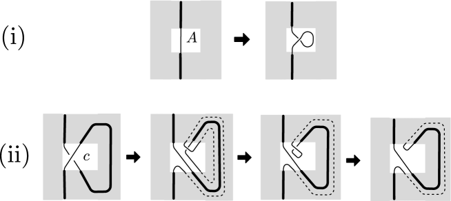
The case of R1. First we consider the case where an R1 move from left to right in Figure 1 is applied. Take a small arc $A$ in $D(L_{1})$ in $M$ and take a small rectangular disk in $M$ , say $\Delta$ , containing $A$ and avoiding $D(L_{2})$ . Apply an R1 move from the left to the right in $\Delta$ as in Figure 6 (i) and we obtain a desired diagram $D^{\prime}$ . (The shaded region is $M\setminus\Delta$ .)

We consider the case where an R1 move from right to left in Figure 1 is applied. Let $c$ be a self crossing of $D(L_{1})$ which is removed by the R1 move. Take a small rectangular region in $M$ , say $\Delta$ , containing $c$ and avoiding $D(L_{2})$ . Apply a sequence of deformation to $D(L_{1})$ as in Figure 6 (ii) and we obtain a desired diagram $D^{\prime}$ . (The shaded region is $M\setminus\Delta$ . The first deformation is an over finger move. The second deformation is an over detour move. The third deformation is an R1 move.)

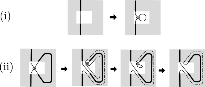
The case of VR1. We consider the case where a VR1 move in Figure 1 is applied. By a similar argument to the case of an R1 move, we have a desired diagram $D^{\prime}$ . See Figure 7. (In (ii), the first deformation is a virtual finger move. The second deformation is a detour move. The third deformation is a VR1 move.)

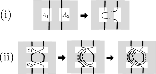
The case of R2. We consider the case where an R2 move from left to right in Figure 1 is applied. Take small arcs $A_{1},A_{2}$ in $D(L_{1})$ and take a pair of small rectangular regions in $M$ , say $\Delta_{1},\Delta_{2}$ containing $A_{1},A_{2}$ and avoiding $D(L_{2})$ as in the left of Figure 8 (i). Applying an over finger move as in Figure 8 (i) and we obtain a desired diagram $D^{\prime}$ . (The shaded region is $M\setminus(\Delta_{1}\cup\Delta_{2})$ .)

We consider the case where an R2 move from right to left in Figure 1 is applied. Let $c_{1},c_{2}$ be self crossings of $D(L_{1})$ which are removed by the R2 move in $M$ . Take small rectangular regions in $M$ , say $\Delta_{1},\Delta_{2}$ , containing $c_{1},c_{2}$ and avoiding $D(L_{2})$ . Apply a sequence of deformation to $D(L_{1})$ as in Figure 8 (ii) and we obtain a desired diagram $D^{\prime}$ . (The first deformation is an under finger move. The second deformation is an over detour move.)

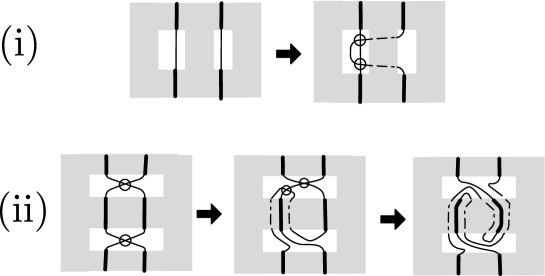
The case of VR2. By a similar argument to the case of R2, we have a desired diagram $D^{\prime}$ . See Figure 9. (In (i), the deformation is a virtual finger move. In (ii), the first deformation is a virtual finger move. The second deformation is a detour move.)

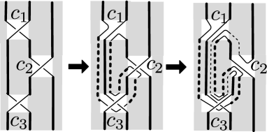
The case of R3. We consider the case where an R3 move from left to right in Figure 1 is applied. Let $c_{1},c_{2}$ and $c_{3}$ be the three crossings of $D(L_{1})$ where the R3 move is applied, and take small rectangular regions in $M$ , say say $\Delta_{1},\Delta_{2},\Delta_{3}$ , containing $c_{1},c_{2},c_{3}$ and avoiding $D(L_{2})$ . Apply a sequence of deformation to $D(L_{1})$ as in Figure 10 and we obtain a desired diagram $D^{\prime}$ . (The shaded region is $M\setminus(\Delta_{1}\cup\Delta_{2}\cup\Delta_{3})$ . The first deformation is a consecutive application of two under finger moves. The second deformation is an over detour move.)

An R3 move from right to left is not necessary, since it is obtained from an R3 move from left to right by rotating the figure by 180 degree.

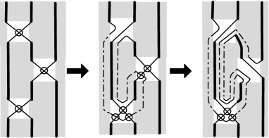
The case of VR3. We consider the case where a VR3 move from left to right in Figure 1 is applied. Apply a sequence of deformation to $D(L_{1})$ as in Figure 11 and we obtain a desired diagram $D^{\prime}$ . (The first deformation is a consecutive application of two virtual finger moves. The second deformation is a detour move.) A VR3 move from right to left is not necessary.

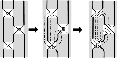
The case of VR4. We consider the case where an VR4 move from left to right in Figure 1 is applied. Apply a sequence of deformation to $D(L_{1})$ as in Figure 12 and we obtain a desired diagram $D^{\prime}$ . (The first deformation is a consecutive application of two virtual finger moves. The second deformation is a detour move.) A VR4 move from right to left is not necessary.

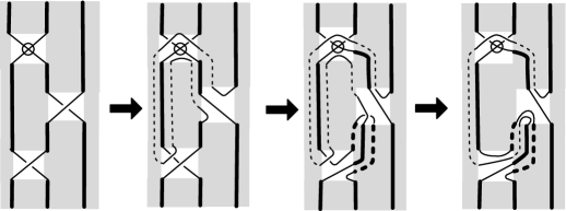
The case of WR. We consider the case where an WR move from left to right in Figure 1 is applied. Apply a sequence of deformation to $D(L_{1})$ as in Figure 13 and we obtain a desired diagram $D^{\prime}$ . (The first deformation is a consecutive application of two over finger move. The second deformation is an under finger move. The third deformation is an over detour move.) A WR move from right to left is not necessary. $\square$

Lemma 5.

Let $D$ be a diagram of a welded link $L$ partitioned into $L_{1}$ and $L_{2}$ . Let $D_{1}$ be a diagram of $L_{1}$ . There is a diagram $D^{\prime}$ of $L$ such that $D^{\prime}(L_{1})$ is isotopic to $D_{1}$ in $\mathbb{R}^{2}$ and $D^{\prime}(L_{2})=D(L_{2})$ .

Proof.

Using Lemma 4 inductively, we obtain the result. $\square$

Proof of Theorem 2.

Suppose that $D_{1},\dots,D_{n}$ are welded link diagrams. Let $L$ be a welded link partitioned into sublinks $L_{1},\dots,L_{n}$ admitting diagrams $D_{1},\dots,D_{n}$ respectively.

Let $D=D^{(0)}$ be a diagram of $L$ . By considering $L$ to be partitioned into $L_{1}$ and $L\setminus L_{1}$ and applying Lemma 5, there is a diagram $D^{(1)}$ of $L$ such that $D^{(0)}(L_{1})$ is isotopic to $D^{(1)}(L_{1})$ and $D^{(0)}(L\setminus L_{1})=D^{(1)}(L\setminus L_{1})$ .

Inductively, for $i=2,\dots,n$ , assume that we have a diagram $D^{(i-1)}$ . By considering $L$ to be partitioned into $L_{i}$ and $L\setminus L_{i}$ and applying Lemma 5, there is a diagram $D^{(i)}$ of $L$ such that $D^{(i-1)}(L_{i})$ is isotopic to $D^{(i)}(L_{i})$ and $D^{(i-1)}(L\setminus L_{i})=D^{(i)}(L\setminus L_{i})$ .

Then $D^{\prime}=D^{(n)}$ is a desired diagram. $\square$

4. Proof of Theorem 3

In order to prove Theorem 3, we use the notion of the 2-cyclic covering of a virtual link, introduced in [5, 6].

Let $D$ be a diagram. Moving $D$ by an isotopy of $\mathbb{R}^{2}$ , we assume that $D$ is on the left of the $y$ -axis and all crossings have distinct $y$ -coordinates. Let $D^{*}$ be a copy of $D$ on the right of the $y$ -axis which is obtained from $D$ by sliding along the $x$ -axis. Let $v_{1},\dots,v_{k}$ be the virtual crossings of $D$ and let $v^{*}_{1},\dots,v^{*}_{k}$ be the corresponding virtual crossings of $D^{*}$ . For each $i\in\{1,\dots,k\}$ , we denote by $l_{i}$ the horizontal line containing $v_{i}$ and $v_{i}^{*}$ , and let $N(l_{i})$ be a regular neighborhood of $l_{i}$ in $\mathbb{R}^{2}$ . Consider a diagram, denoted by $\widetilde{D}$ , obtained from $D\cup D^{*}$ by replacing the intersection with $N(l_{i})$ for each $i\in\{1,\dots,k\}$ as in Figure 14. We call the diagram $\widetilde{D}$ a 2-cyclic covering diagram of $D$ .

For example, for the diagram $D$ depicted in Figure 15 (i), the diagram $D\cup D^{*}$ is as in (ii). Then we have a 2-cyclic covering diagram $\widetilde{D}$ as in (iii).

Theorem 6 ([5, 6]).

Let $D$ and $D^{\prime}$ be diagrams. If $D$ is equivalent to $D^{\prime}$ as a virtual link, $\widetilde{D}$ is equivalent to $\widetilde{D^{\prime}}$ as a virtual link.

Refer to [5, 6] for details. By this theorem, the 2-cyclic covering is defined for a virtual link. For a virtual link $L$ , the 2-cyclic covering of $L$ , denoted by $\widetilde{L}$ , is defined to be the equivalence class of $\widetilde{D}$ for a diagram $D$ of $L$ .

When $L$ is partitioned into $L_{1},\dots,L_{n}$ , then the 2-cyclic covering $\widetilde{L}$ is partitioned into $\widetilde{L}_{1},\dots,\widetilde{L}_{n}$ .

Proof of Theorem 3.

Let $D_{i}$ $(i=1,2)$ be a loop with no crossings. Let $D^{\prime}=D^{\prime}_{1}\cup D^{\prime}_{2}$ be the diagram depicted in Figure 16 (i), and let $L$ be a virtual link presented by $D$ which is partitioned into $L_{1}$ and $L_{2}$ with $D^{\prime}(L_{i})=D^{\prime}_{i}$ $(i=1,2)$ . We assert that there is no diagram $D$ of $L$ such that the restriction $D(L_{i})$ to $L_{i}$ is isotopic to $D_{i}$ for $i=1,2$ .

Suppose that there is a diagram $D$ of $L$ such that the restriction $D(L_{i})$ to $L_{i}$ is isotopic to $D_{i}$ for $i=1,2$ . Consider a 2-cyclic covering diagram $\widetilde{D}$ of $D$ and let $\widetilde{D}=\widetilde{D}_{1}\cup\widetilde{D}_{2}$ . The diagram $\widetilde{D}_{i}$ presents the sublink $\widetilde{L}_{i}$ for $i=1,2$ .

Consider a 2-cyclic covering diagram $\widetilde{D^{\prime}}$ of $D^{\prime}$ and let $\widetilde{D^{\prime}}=\widetilde{D^{\prime}}_{1}\cup\widetilde{D^{\prime}}_{2}$ . The diagram $\widetilde{D^{\prime}}_{i}$ presents the sublink $\widetilde{L}_{i}$ for $i=1,2$ .

By Theorem 6, the diagram $\widetilde{D}_{i}$ is equivalent to the diagram $\widetilde{D^{\prime}}_{i}$ as a virtual link for $i=1,2$ .

As seen in Figure 16 (ii), the diagram $\widetilde{D^{\prime}}_{1}$ is a diagram consisting of two components with linking number $1$ . (The linking number of a diagram with two components is the sum of signs of classical non-self crossings divided by $2$ . It is an invariant of a virtual link with two components.)

On the other hand, the diagram $\widetilde{D}_{1}$ is a diagram consisting of two components with linking number $0$ . (This is seen as follows: $D_{1}$ is a loop with no crossings, $D_{1}\cup D^{*}_{1}$ is a pair of loops with no crossings. The diagram $\widetilde{D}_{1}$ is obtained from $(D_{1}\cup D_{2})\cup(D^{*}_{1}\cup D^{*}_{2})$ by replacement as in Figure 14, there is no classical crossing on $\widetilde{D}_{1}$ .)

This is a contradiction. $\square$

The proof above shows that there exists a virtual link $L=L_{1}\cup L_{2}$ with two components such that when we forget $L_{2}$ , $L_{1}$ is equivalent to the trivial knot and that for any diagram $D$ of $L$ , the restriction $D(L_{1})$ has at least one crossing.

References

[1] J. S. Carter, S. Kamada and M. Saito, Stable equivalence of knots on surfaces and virtual knot cobordisms, J. Knot Theory Ramifications 11 (2002), 311–322.
[2] R. Fenn, R. Rimanyi, C. Rouke, The braid-permutation group, Topology 36 (1997), 123–135.
[3] J. H. Lee, G. T. Jin, Link diagrams realizing prescribed subdiagram partitions, Kobe J. Math. 18 (2001), 199 – 202.
[4] N. Kamada, On the Jones polynomials of checkerboard colorable virtual knots, Osaka J Math. 39 (2002), 325–333.
[5] N. Kamada, Coherent double coverings of virtual link diagrams, J. Knot Theory Ramifications 27 (2018), 1843004 (18 pages).
[6] N. Kamada, Cyclic covering of virtual link diagrams, Internat. J. Math. 30 (2019), 1950072 (16 pages).
[7] N. Kamada and S. Kamada, Abstract link diagrams and virtual knots, J. Knot Theory Ramifications 9 (2000), 93–106.
[8] L. H. Kauffman, Virtual knot theory, European J. Combin. 20 (1999), 663–690.
[9] S. Satoh and K. Taniguchi, The writhe of a virtual knot, Fundamenta Mathematicae 225(1) (2014), 327–341.