Diamagnetic to paramagnetic oscillations in an exploding Coulomb gas
††preprint: AIP/123-QEDDense positively-charged plasmas generated through the irradiation of particles with high intensity ultrashort laser pulses has been a topic of considerable experimental and theoretical research within the past two decadesKaplan et al. (2003); Kovalev and Bychenkov (2005); Last et al. (1997); Murphy et al. (2014); Degtyareva et al. (1998). Such ultrashort laser pulses can result in the effective removal of electrons from the particles, a process called laser ablation, and if unconfined, the resulting positively ionized particles left behind undergo rapid expansion. Such dynamics has come to be known as Coulomb explosion within the literatureLast et al. (1997); Grech et al. (2011). Analogous Coulomb explosion dynamics can be observed within the probe used in ultrafast electron microscopy (UEM) where a rapidly emitted electron bunch undergoes similar Coulomb-driven free-expansionLuiten et al. (2004); Siwick et al. (2002); Reed (2006); Zerbe et al. (2018). The primary difference between electron and ion dynamics is in their time scale. That is, as electrons are far lighter than ionized atoms or molecules, the dynamics evolve within the ultrafast regime; otherwise, the mathematical description is analogous.
Recently, Coulomb explosion dynamics of an electron single component plasma (SCP) generated within the objective lens magnetic field of a UEM device have been witnessed by both our groupZandi et al. (2020) and othersSun et al. (2020). Due to the presence of the magnetic field, the size of the Coulomb exploding bunch transverse to the magnetic field oscillates while it continues to expand in the longitudinal direction along the magnetic field. We presented a very simple, non-interacting model that adequately captured the dynamics we witnessed in our experiment provided we fit the initial Pearson correlation, or chirp, between the transverse velocity and spatial components to the data; this was justified as such a chirp arises in Coulomb explosions. Operating at higher densities and strong magnetic confinement, Sun et al witnessed evolution of the oscillation frequency in the transverse oscillationsSun et al. (2020); namely, as the expanding electron SCP began to interact with the containment device, the plasma shifted from lower to upper hybrid modes, which are plasma normal modes shifted from the cyclotron frequency due to space-charge effectsJeffries et al. (1983); Heinzen et al. (1991); Dubin (1993).
However, the Coulomb explosion within a magnetic field differs from the situations treated in the trapped plasma literature. Trapped plasmas, especially SCPs, can be maintained for long periods of timeDubin (1996); Danielson et al. (2015). Such plasmas can be described by a rigid-rotor equilibrium where the plasma particles within the plasma collectively rotate similar to a rigid-bodyBogema Jr and Davidson (1970) with an equilibrium distribution determined by the angular momentum and temperature of the plasmaDavidson and Krall (1969). The trapped plasma relatively rapidly approaches such rigid-rotor equilibrium, and therefore substantial attention has focussed on the description of plasma dynamics near this thermal equilibriumJeffries et al. (1983); Dubin (1991); O’neil and Dubin (1998). The period of time during which the plasma is far-from-equilibrium is not as well understood, and the partially unconfined Coulomb explosion is much better described as far-from-equilibrium than is the standard in trapped plasmas.
Nonetheless, there is some understanding of this rapid period of thermalization. Trapped plasmas are known to cool as they approach rigid-rotor equilibrium due to cyclotron radiationO’Neil (1980); Amoretti et al. (2003). The RMS emittance of SCPs used for accelerator beams is known to increase and nearly saturate within the plasma period of the initial distributionStruckmeier et al. (1984), and this change can be attributed to free-energy released from the relaxation of a beam from a non-uniform profile to a nearly-uniform profileWangler et al. (1985); Reiser (1991). Disorder induced heating (DIH) exhibits similar dynamics to RMS emittance evolutionMaxson et al. (2013) although the origin of the free-energy in DIH has been described as quantum or stochasticGericke and Murillo (2003); Murillo (2006). Models including additional stochastic effectsStruckmeier (1994, 1996, 2000); Gao (2000), chaotic effectsKandrup et al. (2004), and non-linear field effectsJensen et al. (2014); Dowell and Schmerge (2009); Gevorkyan et al. (2018) have described addittional pieces of similar thermalization processes, and these descriptions inform the use of RMS envelope equations that are widely used by accelerator physicists to model the dynamics of nearly uniform SCPs(for instanceLund et al. (2014)). However, as it is known that the equilibrium distribution significantly deviates from uniform, it is not apparent whithin the literature to what extent a uniform distribution can capture the dyanmics of Coulomb-explosion within a magentic field.
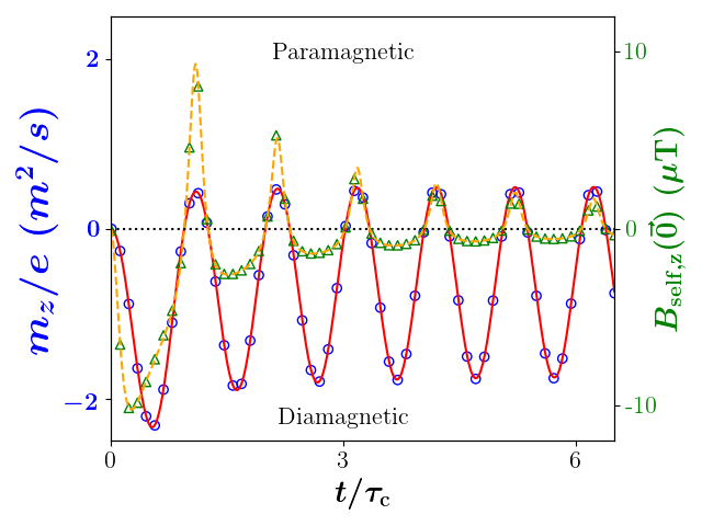
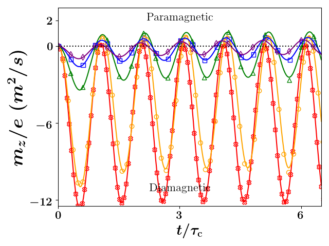
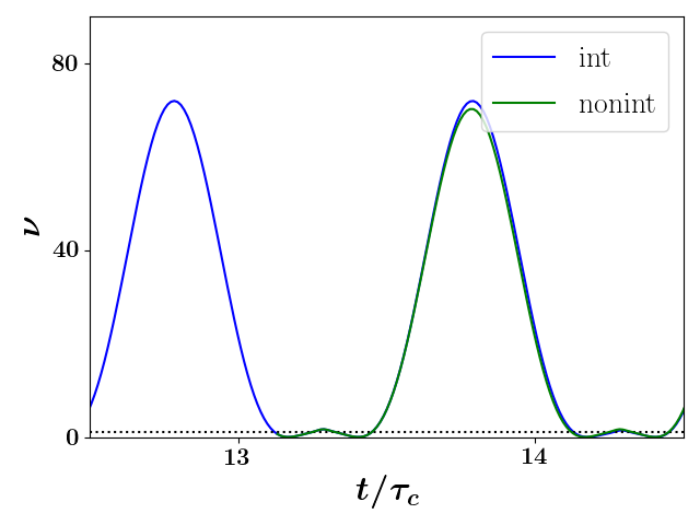
In our previous work, we developed a non-interacting, RMS envelope model. We initialized this model with a non-zero Pearson correlation, or chirp, that we argued arose due to the action of Coulomb explosionZandi et al. (2020), and we found that this model captured the dynamics adequately for our experimental purposes. On the other hand, the frequency shifts seen in Sun et al’s experiments suggests that particle-particle interactions need to be considered, and when we conducted -particle simulations of denser plasmas, we were surprised to see a fundamental effect that appears to be missing in the trapped plasma and accelerator literatures — transversely confined Coulomb explosion can lead to the self-magnetic moment of the electron SCP flipping its sign and driving the SCP into a paramagnetic state. We demonstrate this effect in Fig. 1 where we show the magnetic moment changes sign twice every period. This signals a periodic transition between paramagnetic and diamagnetic states for the Coulomb exploding electron SCP despite this ensemble starting with no appreciable angular momentum.
In this paper, we demonstrate this effect with -particle results, show how increasing the magnetic field effectively turns this effect on, show how “heating” of the electron SCP results in the elimination of the paramagnetic portion of the oscillation, and present three very simple models streamlined from existing accelerator literature that can be used to understand the diamagnetic to paramagnetic oscillation and this temperature effect. Further, we introduce two novel physical measures: (1) a rigid-rotor statistic and (2) an angular emittance measure. As we could not find a quantitative definition of rigid-rotor motion, we present such a measure with the rigid-rotor statistic. In the development of this statistic, we found a statistical expression that is nearly conserved in time for non-interacting systems and appears to be the angular complement to the radial emittance proposed by othersLund et al. (2014). We summarize and place these results in context of the literature in the Conclusions.
I -particle simulations and spheroidal envelope equations from rest
We examined the dynamics of electron SCPs exploding from rest within a uniform magnetic field strength of over a wide variety of initial conditions (not shown) using -particle simulations, and compared the -particle results to envelope equations. We term the direction along the magnetic field axis the longitudinal direction and the two directions perpendicular to this direction the transverse direction(s). -particle simulations were carried out using the Velocity-Verlet algorithmVerlet (1967) with the electric field calculated using the Fast Multipole MethodGimbutas and Greengard (2015) at every step.
Before discussing specific results, we briefly introduce our spheroidal envelope model and notation. For simplicity, we assumed cylindrical symmetry (perfect Pearson correlation between and ), with representing the transverse “radial” variance, with representing the variance along and the longitudinal standard deviation; the parameters and are often termed the RMS envelope of the SCP as we will do here. Under the assumption of perfect Pearson correlation between and and no Pearson correlation with , we define the radial (), angular (), and longitudinal () chirps by the line of best fit for the velocity, i.e. , where represents the covariance of and , etc. We use tilde above a parameter to indicate the dimensionless version of the parameter and in the subscript to indicate its initial value. The analysis can be made dimensionless by scaling the spatial length by the appropriate initial length and the time by the electron’s cyclotron frequency associated with the external magnetic field where is the elementary charge and is the mass of the electron. Three examples of this are , , and . The resulting dimensionless system of equations describing the evolution of the phase space coordinates starting from rest follows:
| (1a) | ||||
| (1b) | ||||
| (1c) | ||||
| (1d) | ||||
| (1e) | ||||
where is the initial plasma frequency of the SCP (in three dimensions, hence the p in the subscript), is the aspect ratio, and and are functions that determine the effect geometry has on the force. We provide a fluid derivation of this system of equations in Section XXX of the supplemental. Similar envelope models are well established in the literatureLund et al. (2014); in fact, the philosophy for presenting this model here is to have minimal complexity for understanding the physics while maintaining the agreement between the model and the dynamics of the situation.
We note that Eq. (1d) is not typically reported as part of the envelope equations; however, equivalent forms of this expression can be found in the literature describing the equilibrium distribution of SCPs (for instance, Eq. (5.36) ofReiser (1994)). This equation is always derived from a consideration of the conservation of angular momentum, as we have done in Section XXX of the supplement. However, our use of this equation is somewhat different from the standard use. In most cases where this equation may be found, the researcher is looking at a plasma at equilibrium. Therefore, in addition to Eq. (1d), equilibrium analyses also assume is constant in time, i.e. and or more generally . Substantial effort has been made to describe such distributions of interacting SCPs using these constraints [refs]; namely, we know “equilibrium beams” satisfies Eq. (1d) and a constant by adopting a non-uniform profile when the generalized angular momentum is non-zeroBogema Jr and Davidson (1970). However, this well-established observation need not necessarily be true for far-from-equilibrium SCPs and beams. Namely, if the radius is not constant, the distribution may be undergoing oscillations while remaining nearly uniform. We examine this possibly controversial statement further in the next section.
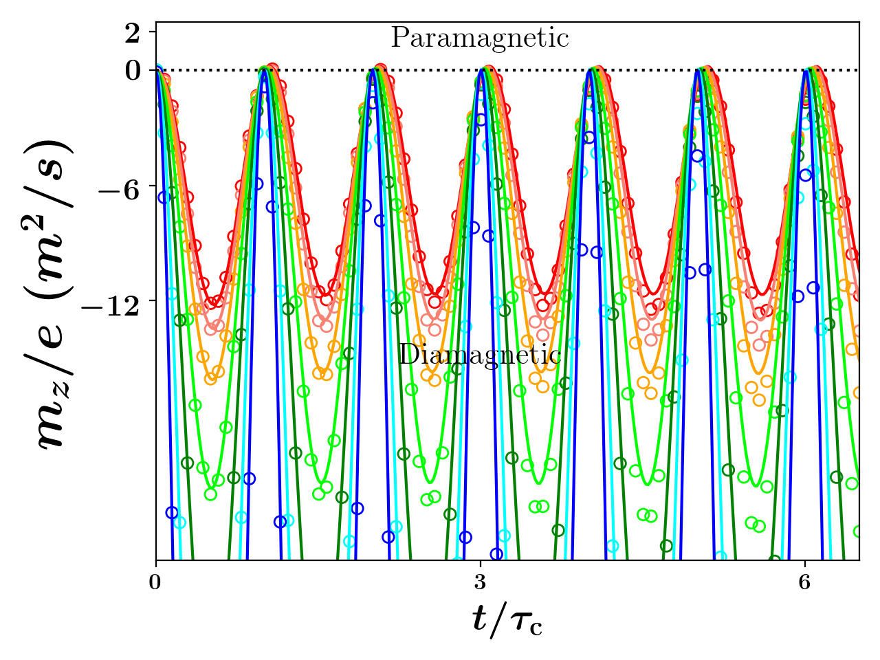
For our first representative simulation, we initialized electrons with spatial coordinates sampled from a spherical-uniform distribution with radius m and evolved this distribution from rest under the influence of the particles’ pair-wise repulsion and an external magnetic field strength of T. Fig. 1 shows the evolution of the longitudinal magnetic moment from both the -particle simulation and the envelope equations starting from rest. As can be seen, the -particle results and envelope prediction are in near perfect agreement. As the longitudinal magnetic moment reverses direction twice during every oscillation, the magnetic moment is aligned with the external magnetic field, i.e. is diamagnetic, and opposite to the external magnetic field, i.e. is paramagnetic, for periodic intervals during this oscillation. We note this oscillation is consistent with the Bohr-Van Leeuwen theoremVan Leeuwen (1921) as our system is far-from-equilibrium; likewise, it is not inconsistent with the standard attribution of magnetically confined plasmas as being diamagneticO’Neil (1995) as such a description again assumes equilibrium-like conditions.
As the longitudinal magnetic moment, , in our notation is given by
| (2) |
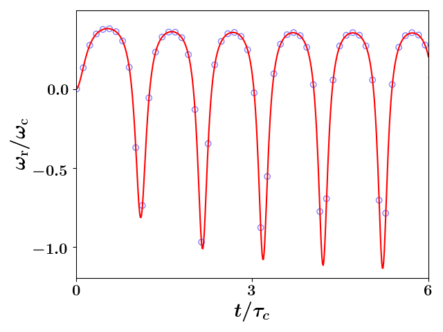
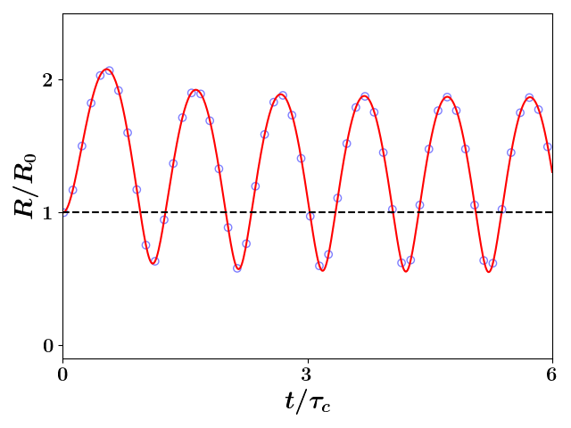
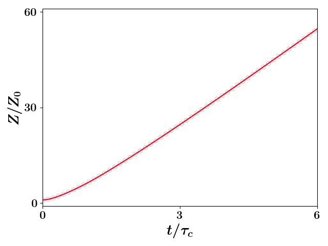
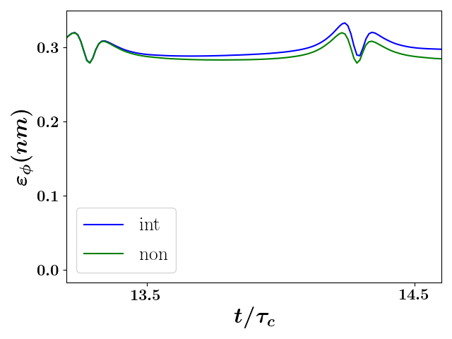
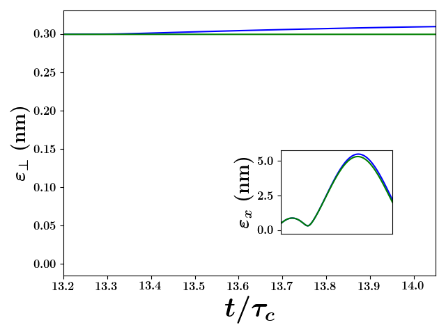
we see that the sign of the magnetic moment of the SCP is determined by the direction of rotation captured by the angular chirp. The oscillation of the angular chirp for our first characteristic simulation is displayed in Fig. 2a; again, these results are in excellent agreement. As the radial motion is captured in the model through the evolution of the parameter , which is the sole time-dependent parameter in Eq. (1d), we see that couples to the radial dynamics so that and oscillate at the same frequency. The envelope predicted and -particle simulated oscillation of and the unbound expansion of are seen in Figs. 2b and 2c, respectively. Notice is negative for any value of that is less than for simulations starting from rest; that is, the transition between the diamagnetic and paramagnetic states occurs when the transverse radius crosses its original size as can be seen by comparing Figs. 1 or 2a with Fig. 2b. We note that the evolution of seen in Fig. 2c is typical of unconfined Coulomb explosion; namely, the rapid acceleration of the growth in the statistic followed by a period of almost linear growth leading to a consistent decrease in the density and hence a weakening of space charge effects.
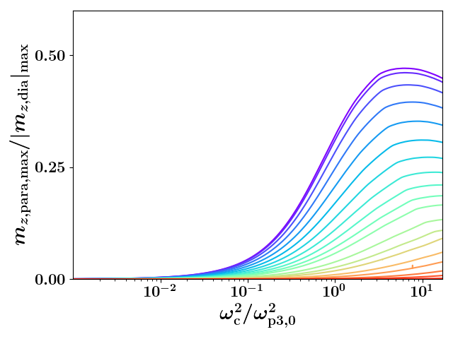
As this effect is in and the expanding longitudinal dimension results in a highly dynamic density, it is not apparent that this effect is the same for every magnetic field. As the only frequencies relative to this situation are the cyclotron and plasma frequencies, we consider this effect as a function of . In Fig. 3a, we show how the oscillatory dynamics respond to changes in when all other parameters are held constant. The amplitude of the oscillations decreases as the ratio between the frequencies is increased; interestingly, though, the size of the oscillation’s amplitude within the paramagnetic regime increases to a point at which further increasing of the magnetic field likewise begins to decrease the size of the oscillation in the paramagnetic region. In other words, at very low values of , the self-magnetic field oscillation does not enter very far into the paramagnetic region and such oscillation is effectively turned on by increasing the magnetic field.
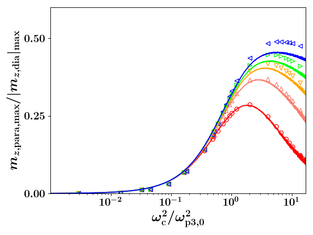
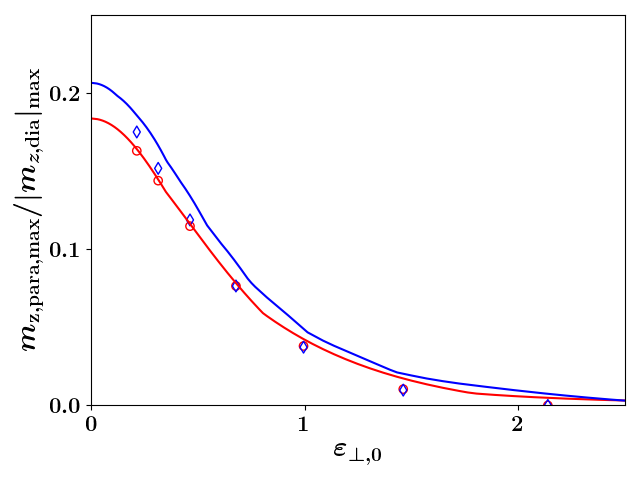
To obtain better intuition into this effect, we quantified the relative size of the paramagnetic and diamagnetic oscillations by looking at the ratio of the minimum to the maximum self-magnetic moments, i.e. . As can be seen in Fig. 3a, the fist diamagnetic peak is somewhat larger than subsequent peaks, so this ratio in our envelope treatment effectively uses the size of this first peak in the diamagnetic region to gauge the size of the subsequent peaks in the paramagnetic region. Moreover, the subsequent peaks within the paramagnetic region slowly increase toward an asymptote as can be seen in Fig. 3b — this is due to the SCP becoming less and less dense as it expands longitudinally resulting in the space-charge effect becoming less and less important in determining where the oscillating SCP will reverse its inward motion. On the other hand, as we increase the magnetic field, the number of oscillations occuring before the space-charge effect becomes negligible increases. As we are comparing simulation results at the same multiple of the the cyclotron period, this means that it takes the space-charge effect will emerge later in simulation with relative larger cyclotron frequencies. This is the origin of the peak seen in Fig. 3a.
As can be seen, increasing the ratio does appear to turn this oscillation on — specifically, the turning on occurs when is in the range . Note that the “Brillouin point” occurs when the initial angular motion is rotating at and , but here there is no initial angular motion and the oscillation is driven entirely by the initial expansion of the electron SCP; therefore, the occurence of in this range is unrelated to the Brillouin point.
Comparing the results of the RMS envelope equations to the -particle simulations, the general trends are captured by the model in both Figs. 3a and 3b and are almost exact at earlier times. Notice that the deviations in the ratio monotonically increase during the simulation and are larger for stronger external magnetic fields, and a close inspection of the magnetic moment oscillation for higher magenetic fields can be seen in Fig. 3a. Coincidentally, these are the cases that have larger emittance growth, so we infer these deviations are due to accumulated emittance growth that are not included in Eqs. (1). We will model the effect of RMS emittance in this situation in a later section, but such treatment will still consider the emittance as being conserved — just non-zero — but still not dynamic as it is in the simulations.
II Rigid-rotor non-equilibrium and emittance-induced shear
As mentioned in the previous section, substantial work has been done to describe the steady-state properties of confined plasmas[refs]. Initial work by Brillouin described a uniform steady-state where the angular chirp is given by the Larmor frequency, Brillouin (1945), and subsequent work has extended this understanding to non-uniform steady-state distributions rotating with angular chirps in the range known as rigid-rotor equilibrium.
To our knowledge, there is no clear quantitative definition of rigid-rotor equilibrium; so we develop one here. If we were to calculate the angular kinetic energy of a rigid-rotor, we would expect that the amount of angular kinetic energy predicted by the linear chirp, i.e. , should be much larger than the amount of angular kinetic energy associated with random motions. Consider the angular velocity of the particle, . We know that the residual for the particle between the chirp-predicted and measured angular velocity can be written as
| (3) |
where and are the radial and angular velocity coordinates for particle . Therefore the variance of the residuals can be written as
| (4) |
Note that as for all whereas and are approximately . As represents the portion of the kinetic energy that is associated with motions that are not linearly correlated and is often attributed to being random, it follows that the ratio
| (5) |
can quantify the rigid-rotor approximation; we call the rigid-rotor statistic. Indeed if the rigid-rotor statistic is larger than , the majority of the angular kinetic energy is associated with the motion described by the angular chirp.
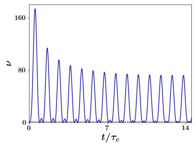
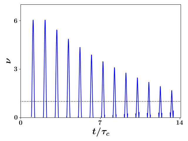
For a second characteristic simulation, we show the rigid-rotor statistic as a function of time in Fig. 4a. This second simulation again had electrons but was initially sampled from the spherical uniform distribution with initial radius m from rest with a magnetic field strength of T. As can be seen in this figure, the rigid-rotor statistic is much larger than except when it crosses at which time the SCP is in the process of reversing its direction of rotation; at this time, the angular chirp is zero and therefore the kinetic energy associated with the coherent portion of the rotation captured by this statistic is zero as well. Such dynamics should not be described as rigid-rotor-like. However, as the radius continues to decrease, the angular chirp becomes negative and the rigid-rotor statistic once again become greater than . This means the distribution begins to rigidly rotate in the opposite direction after briefly passing through a state dominated by random angular motion. Due partially to the fact that the expansion beyond is relatively much larger than the contraction within , the rigid-rotor statistic for this latter region does not get as large. Moreover, the rate at which the rigid rotor statistic evolves within the larger than and smaller than regions differ as can be seen in Figs. 4a and 4b.
It is unclear from -particle simulations alone to what extent each of non-zero emittance, space-charge, and emittance evolution effects contribute to evolution of the rigid-rotor statitics seen in Fig. 4a especially once the SCP has expanded significantly. To obtain insight into such dynamics, we re-simulated the last two transverse oscillations without inter-particle forces starting with the same configuration produced from the interacting simulation of Coulomb explosion. We show the comparison between the results of these non-interacting and interacting simulations in Fig. 4c. We note that the evolution of the rigid-rotor statitic is very similar in both cases suggesting that non-interacting-like behavior dominates towards the end of the transverse oscillations; such behavior would also suggest that emittance growth is responsible for the small deviations. On the other hand, we would expect that emittance effects should dampen the rigid-rotor statistic, but what is seen is the opposite — that is, the rigid-rotor statistic for the interacting simulation is larger than the non-interacting simulation.
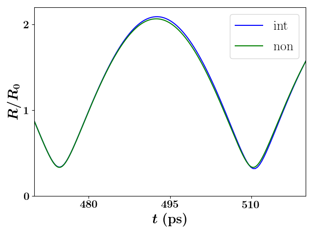
As the rigid-rotor statistic is correlated with the transverse radius of the SCP, one explanation for this effect could be if the interacting simulation were to obtain a larger radius than the non-interacting simulation thus affecting the numerator of the rigid-rotor statistic. In Fig. 5a, the evolution of the non-interacting and interacting radii are shown. As can be seen, the simulated SCP with no interaction predicts a less extreme transverse oscillation. Thus this explanation is consistent with the observed difference between the maxima of the rigid-rotor statistics in Fig. 5c; however, a small deviation is also observed at the minimum radius, and the rigid-rotor statistic does not display the complementary deviation in the rigid-rotor statistic during this time period. So something more is going on near the transverse minima that compensates for the radial effect seen at the maximum.
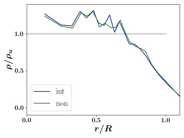
We explored the densities predicted near the final simulated transverse minimum to understand if a space-charge shift in the bunch profile could be compensating for the radial-induced expected deviation near the minima. As the second-order moments are sensitive to profile changes, such a profile change should result in a change in the rigid-rotor statistic that we would then attribute to the use of second order moments. We show the transverse radial density at the transverse radial minimum for both simulations in Fig. 5b. As can be seen, the simulated radial densities do in fact deviate substantially from the theoretically uniform distribution, but they do not deviate from one another. Specifically, a clear edge effect that is well discussed in the equilibrium literature [refs] arises when the bunch reaches its minimum transverse radius, but again, this occurs in both the interacting and non-interacting simulations. Therefore, this density effect cannot be causing the difference in the rigid-rotor statistic. Further, as the only portion of the non-interacting dynamics that is driving distribution change is the emittance, we conclude that the edge effect is solely an emittance effect in both cases.
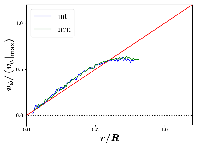
A second possible mode of compensation would be if our statistical estimate of the kinetic energy in the angular mode from the angular chirp could differ between the two simulations if non-linearities were to arise. We show the angular phase-space at the transverse radial minimum for both simulations in Fig. 5c. As in the radial density, a clear edge effect, which could be described as a shear, can be seen; however, again the same effect is seen in both the interacting and non-interacting simulations. Therefore, we conclude that the compensation in the rigid-rotor statistic is not driven by this shear effect and further that the shear is likewise a result of emittance.
A third possible compensatory mechanism is if the denominator in Eq. (5) were to somehow differ between the two simulations. To examine this denominator, we point out that normalized RMS emittance, standardly defined [refs] as
| (6) |
and defined transversely in the presence of cylindrical-symmetry about a magnetic field byLund et al. (2014)
| (7) |
is effectively the velocity spread times the spatial spread when the bunch is projected to a single dimension [refs]. Therefore, we multiplied the velocity spread, or the square root of the residual variance from Eq. (4), by to define an “angular emittance”,
| (8) |
As can be seen in Fig. 6a, this measure is very roughly conserved during the non-interacting simulation. Interestingly, it is also roughly the same value as the cylindrically-symmetric emittance seen in Fig. 6b. The small emittance growth seen in both the angular and transverse emittances appears to contribute to the fact that the rigid-rotor statistic is smaller at the minimum of the transverse width than should be expected from the evolution of the radius alone.
We note that this roughly conserved angular emittance has not been described in the literature but can be argued to be the complement of the round-beam thermal emittance defined by Lund et alLund et al. (2014) presented in Eq. (7). Also interestingly, obtaining the Cartestian covariances and re-sampling the distribution to make an equivalent initial condition [not shown] neither captures the correct angular emittance nor the evolution of the rigid-rotor statistic. This suggests that the standard statistics are not capturing all of the spatial correlations present in the SCP.
III Effect of non-zero emittance on magnetic state reversal in simulations
We now consider cases where the SCP starts with some temperature, which we quantify by the dimensionless emittances defined by
| (9a) | ||||
| (9b) | ||||
where is a dimensionless version of Eq. (7). Following the formulation of the envelope equations by Lund et alLund et al. (2014), we add standard definitions of emittance to our equations with the additional assumption that we are starting with non-zero angular motion, , resulting in changes to Eqs. (1c), (1d), (1e):
| (10a) | ||||
| (10b) | ||||
| (10c) | ||||
Our addition of the transverse and longitudinal emittance terms can be argued analogous to Lund et al. or derived completely from a statistic standpoint (in preparation); angular emittance is not added to Eq. (10b) as the equation is a statement of conservation of angular momentum. The addition of the dimensionless normalized RMS emittance terms captures the effect of motion that deviates from the linear chirps, sometimes described as thermal effects [refs], that result in an outward-like force on the RMS envelope parameters. This is analogous to temperature pressure in fluid models [refs], but is formulated from a discrete statistical vantage point where no theoretical approximations are needed.
To examine the effect of the emittance on the diamagnetic/paramagnetic oscillation, we conducted -particle simulations of initially spherically symmetric Coulomb explosion, initially with , and integrated the envelope equations. For the initial conditions we held fixed and varied . The evolution of some such characteristic simulations can be seen in Fig. 7a. What is apparent is that increasing the initial emittance leads to larger oscillations, shifts the frequency of oscillations higher and decreases the size and duration of the magnetic moment within the paramagnetic region — in a way, this is nearly the opposite of the effect of increasing the confining magnetic field. A plot of the ratio of the maximum self-magnetic moments in each region with such initial conditions viewed as a function of can be seen in Fig. 7b. The envelope data is shifted rightward relative to the -particle simulated data as the -particle simulations undergo disorder induced heating that increases the emittance. As can clearly be seen, increasing the dimensionless emittance beyond about 0.1 decreases the paramagnetic/diamagnetic statistic, and the effect is again turned off once the dimensionless emittance is increased past about 2.
Our envelope model predicts the behavior of the -particle simulation well especially before the emittance has grown significantly. We have also produced a figure detailing the interaction between and the emittance using just the envelope predictions within the first plasma periods. The competitive nature of these two effects can be seen in Fig. 8; namely, an increase in the emittance requires larger values of before a substantial paramagentic state is observable. Further, increasing the emittance delays at what ratio of this effect arises as can be seen by the fact that the curves with significant emittance in Fig. 8 appear to be scaled versions of the successive evolution of this statistic seen in Fig. 3b. As this delay enables additional effects, like cyclotron radiation and other electromagentic effects, outside of the scope of this paper to occur and further drive the SCP toward equilibrium, sufficiently large emittance will effectively turn this effect off.
So far, our analysis has been principally of numerical results. The spheroidal envelope model does not have an exact analytical solution; however, simpler models do allow more analysis. If we were to match such a model to an experiment where the space charge effect remained important even once the bunch had become significantly oblate, it would require us to fit the initial parameters of the model to the parameters observed analogous to our non-interacting treatment. We analyze this continuous-beam model.
The continuous model is very similar to the spheroidal model. The principal differences are: (1) there is no longitudinal dimension to model and (2) the geometric factor is absorbed into the plasma frequency giving a cylindrically symmetric plasma frequency. We denote this new plasma frequency by where is the number density along the length of the beam. The subsequent radial oscillation is determined by
| (11) |
Note the evolution of the angular frequency is only changed by the third dimension only through its dependence on as we assume angular momentum is completely along the axis of symmetry. We note that many equivalent models to this can be found in the literatureDubin (1993); Reiser (1994). While this model depends on three parameters, , , and the initial radial velocity, the freedom to assign the initial phase of the oscillation allows us to set one of the initial velocities, by convention the initial radial velocity, to zero. Thus the properties of the oscillations predicted by this model can be understood within the parameter space when is held fixed, and we will conduct our analysis within this parameter space for various values of .
We note that this parameter space is standard in descriptions of rigid-rotor equilibria; namely, this parameter space is typically used to visualize the parabola of zeros of the effective force that describe the well known rigid-rotor equilibriaGould (1995). In the accelerator literature where continuous beam behavior near rigid-rotor states is discussed, small radial oscillations about a rigid-rotor equilibrium are described as RMS-mismatched induced transverse ripples along the longitudinal coordinateReiser (1994); however, such descriptions focus solely on the effect of and not its coupling to , which we emphasize as being important here.
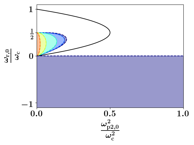
A diagram denoting all of the regions of parameter space where the initial conditions of the continuous-beam model will experience the phase transition for various values of is displayed in Fig. 9. One interesting aspect of this diagram is the fact that the two shaded regions, one inside the rigid-rotor parabola and a second describing the half-plane with , describe the same oscillations. That is, our convention of no initial radial velocity is ambiguous as there exists two times per period with zero radial velocity: (1) the time where the radius is maximum (corresponding to the entire region of parameter space inside the rigid-rotor parabola) and (2) the time at which the radius is minimum (that region’s complement). Deducing the fact that all initial conditions within the half plane where produce the paramagnetic oscillations is simple; we know that the point in the oscillation that corresponds to the maximum radius is inside the parabola and has , so all such initial states in this region must change their direction of rotation at some time. The initial states within the rigid-rotor equilibrium parabola that experience the phase transition requires more analysis, and we present the mathematical description of this region’s boundary in Section VI of the supplement.
IV Discussion
We have described the dynamics of Coulomb explosion of an electron SCP within a magnetic field where we have found that the rotation of the SCP can spontaneously reverse direction due to a combination of the space-charge effect and the conservation of angular momentum. This reversal of the rotational direction of the SCP results in the SCP periodically switching between diamagnetic and paramagnetic states. This observation is surprising given the established diamagnetic nature of SCPs in ubiquitous Brillouin flow models. We showed that this behavior is turned on by increasing the magnetic field, and turned off by increasing the emittance or thermal kinetic energy in the SCP. Moreover, we showed that this behavior arises from coupling between the radial and angular motion introduced by the magnetic field, and presented equations that describe this coupling. We modeled the radial and hence angular motion of such SCPs with mean-field particle-particle interactions through envelope equations and showed that the envelope equations captures the angular dynamics to the same extent that the radial dynamics are captured.
It is clear that SCPs particularly in traps rapidly evolve toward an equilibrium distribution. During this time, the plasma typically undergoes disorder induced heatingMurillo (2006) as well as cooling through cyclotron radiationO’Neil (1980). However, a full kinetic picture of how such a plasma evolves from a possibly far-from-equilibrium initial state with substantial inter-particle correlation to the eventual equilibrium distribution where particle inter-particle correlations are treated randomly is not apparent within the literature. Our Coulomb explosion model provides insight into some possible early dynamics that could further evolve the inter-particle correlations if relativistic effects were to be properly considered in future work.
We note the parameters we use have statistical definitions. We have been calling the description of the evolution of such parameters statistical kinematics although they are sometimes known as moment equations in the literatureSacherer (1971). These statistical definitions have the benefit of being applicable to arbitrary distributions; in this work, this is true for the radial measure, , angular measure, , and magnetic moment, . However, to capture the time dependence of one of these parameters, specifically the radial measure, we needed to apply mean field theory using the uniform distribution to avoid space-charge non-linearities for which general techniques have yet to been developed. So despite the fact that Eq. (1d) relates the dependence of on in any generic distribution, we can only capture the time evolution through the use of the uniform distribution for which an analytic expression for the space-charge force is available.
The insight into the radial/angular coupling adjusts the typical depiction of the SCP breathing mode as a periodic inward and outward motionDubin and Schiffer (1996). Instead, we’ve shown that the angular motion oscillates coherently with the radial motion. That is, instead of moving in and out, the SCP also rotates with rate of the rotation specified by the size of the radius. The microscopic origin of this is of course the cyclotron motion of the particles, and we have provided a simplified schematic of this motion for the non-interacting distribution in the supplemental documentation.
The fundamental theory can be tested experimentally by careful accounting for the mechanical angular momentum of a beam. We note that generalized Courant-Snyder theoryQin et al. (2013) provides tools to track the rotation angle of the envelope matrix in the presence of transverse-coupled dynamics, and this rotation can alternatively be conceptualized as the angular momentum of the beam as we’ve done here. Therefore, that theory and the tools we present here may be used to do such accounting. More specifically, a long solenoid can be used to introduce mechanical angular motion to a prolate SCP in an accelerator setting; the amount of angular momentum can be determined using Eq. (1d) and (11) and knowledge of the angular momentum kick across the solenoid’s fringe. As the SCP evolves in a region without a magnetic field, these equations may again be employed with and the introduced from the solenoid. The SCP could then be passed through a second long solenoid. By tuning the length of the first solenoid, the magnetic field strengths, and the separation distance between the solenoids for an SCP of a known length and number of electrons, it should be possible to induce a near equilibrium SCP once it enters the second solenoid.
V Methods
V.1 Analytic models
We derived the analytic model both from a fluid and from a statistical perspective. Analytic results were compared in order to confirm the accuracy of the derivation and our understanding of the physics. Details of the analytic fluid derivation of the model are provided in the supplement.
V.2 Numerical simulations
We conducted -particle simulations and numerically integrated the envelope equations (Eqs. (11) and (1)).
For the -particle simulations, spatial coordinates were sampled from the specified initial distribution and propagated using Velocity Verlet algorithmVerlet (1967) with the self field determined by the Fast Multipole Method algorithmGimbutas and Greengard (2015) or set to zero (for the non-interacting simulations). Time steps were set to between and . Parameters included:
-
1.
Fig. 1: We simulated (non-interacting) electrons initially uniformly, spherically-symmetrically distributed within the radius m with rotation rate about the axis of an external magnetic field strength of T.
-
2.
Fig. 2: We simulated (non-interacting) electrons initially Gaussian, spherically-symmetrically distributed with standard deviation m with rotation rate about the axis of an external magnetic field strength of T.
-
3.
Fig. 4: We simulated (interacting) an initially spherical electron SCP with electrons uniformly distributed in the radius m starting from rest and undergoing Coulomb explosion within an external magnetic field strength of T, tuned so that the plasma and cyclotron frequencies are comparable.
For the envelope equations, the Velocity Verlet algorithm was again employed for integration. All initial parameters were taken from the initial sample used in the -particle simulations.
VI Acknowledgements
Work by R.M.V. and O.Z. was in part supported by a Packard Fellowship in Science and Engineering from the David and Lucile Packard Foundation. Work by P.D. and B.Z. was supported by NSF Grant numbers RC1803719 and RC108666.
VII Author contributions
O.Z. first noticed the phase transition. O.Z. and B.Z. developed theoretical model, wrote code, and analyzed the simulation and model data. O.Z., R.M.V., P.M.D., and B.Z. interpreted the data and wrote the manuscript.
VIII Data availability
Data available on request from the authors. Simulation and envelope code available on request from authors.
IX Competing interests
The authors declare no competing interests.
X Additional information
X.1 Supplementary information
is available for this paper as a separate pdf.
X.2 Correspondence
Requests for data or code should be addressed to B.Z.
References
- Kaplan et al. (2003) A. E. Kaplan, B. Y. Dubetsky, and P. L. Shkolnikov, Physical review letters 91, 143401 (2003).
- Kovalev and Bychenkov (2005) V. Kovalev and V. Y. Bychenkov, Journal of Experimental and Theoretical Physics 101, 212 (2005).
- Last et al. (1997) I. Last, I. Schek, and J. Jortner, The Journal of chemical physics 107, 6685 (1997).
- Murphy et al. (2014) D. Murphy, R. Speirs, D. Sheludko, C. Putkunz, A. McCulloch, B. Sparkes, and R. Scholten, Nature communications 5 (2014).
- Degtyareva et al. (1998) V. P. Degtyareva, M. A. Monastyrsky, M. Y. Schelev, and V. A. Tarasov, Optical Engineering 37, 2227 (1998).
- Grech et al. (2011) M. Grech, R. Nuter, A. Mikaberidze, P. Di Cintio, L. Gremillet, E. Lefebvre, U. Saalmann, J. M. Rost, and S. Skupin, Physical Review E 84, 056404 (2011).
- Luiten et al. (2004) O. J. Luiten, S. B. vanderGeer, M. J. deLoos, F. B. Kiewiet, and M. J. vanderWiel, Physical review letters 93, 094802 (2004).
- Siwick et al. (2002) B. J. Siwick, J. R. Dwyer, R. E. Jordan, and R. J. Dwayne Miller, Journal of Applied Physics 92, 1643 (2002).
- Reed (2006) B. W. Reed, Journal of Applied Physics 100, 034916 (2006).
- Zerbe et al. (2018) B. Zerbe, X. Xiang, C.-Y. Ruan, S. Lund, and P. Duxbury, Physical Review Accelerators and Beams 21, 064201 (2018).
- Zandi et al. (2020) O. Zandi, A. E. Sykes, R. D. Cornelius, F. M. Alcorn, B. S. Zerbe, P. M. Duxbury, B. W. Reed, and R. M. van der Veen, Nature Communications 11, 1 (2020).
- Sun et al. (2020) S. Sun, X. Sun, D. Bartles, E. Wozniak, J. Williams, P. Zhang, and C.-Y. Ruan, Structural Dynamics 7, 064301 (2020).
- Jeffries et al. (1983) J. Jeffries, S. Barlow, and G. Dunn, International Journal of Mass Spectrometry and Ion Processes 54, 169 (1983).
- Heinzen et al. (1991) D. Heinzen, J. Bollinger, F. Moore, W. M. Itano, and D. Wineland, Physical review letters 66, 2080 (1991).
- Dubin (1993) D. Dubin, Physics of Fluids B: Plasma Physics 5, 295 (1993).
- Dubin (1996) D. H. Dubin, Physical Review E 53, 5268 (1996).
- Danielson et al. (2015) J. Danielson, D. Dubin, R. Greaves, and C. Surko, Reviews of Modern Physics 87, 247 (2015).
- Bogema Jr and Davidson (1970) B. L. Bogema Jr and R. C. Davidson, The Physics of Fluids 13, 2772 (1970).
- Davidson and Krall (1969) R. C. Davidson and N. A. Krall, Physical Review Letters 22, 833 (1969).
- Dubin (1991) D. H. Dubin, Physical review letters 66, 2076 (1991).
- O’neil and Dubin (1998) T. O’neil and D. H. Dubin, Physics of Plasmas 5, 2163 (1998).
- O’Neil (1980) T. O’Neil, The Physics of Fluids 23, 725 (1980).
- Amoretti et al. (2003) M. Amoretti, G. Bonomi, A. Bouchta, P. Bowe, C. Carraro, C. Cesar, M. Charlton, M. Doser, A. Fontana, M. Fujiwara, et al., Physics of Plasmas 10, 3056 (2003).
- Struckmeier et al. (1984) J. Struckmeier, M. Reiser, and J. Klabunde, Part. Accel. 15, 47 (1984).
- Wangler et al. (1985) T. Wangler, K. Crandall, R. Mills, and M. Reiser, IEEE Transactions on Nuclear Science 32, 2196 (1985).
- Reiser (1991) M. Reiser, Journal of applied physics 70, 1919 (1991).
- Maxson et al. (2013) J. Maxson, I. Bazarov, W. Wan, H. Padmore, and C. Coleman-Smith, New Journal of Physics 15, 103024 (2013).
- Gericke and Murillo (2003) D. Gericke and M. Murillo, Contributions to Plasma Physics 43, 298 (2003).
- Murillo (2006) M. S. Murillo, Physical review letters 96, 165001 (2006).
- Struckmeier (1994) J. Struckmeier, Part. Accel. 45, 229 (1994).
- Struckmeier (1996) J. Struckmeier, Physical Review E 54, 830 (1996).
- Struckmeier (2000) J. Struckmeier, Physical Review Special Topics-Accelerators and Beams 3, 034202 (2000).
- Gao (2000) J. Gao, Nuclear Instruments and Methods in Physics Research Section A: Accelerators, Spectrometers, Detectors and Associated Equipment 441, 314 (2000).
- Kandrup et al. (2004) H. E. Kandrup, I. V. Sideris, and C. L. Bohn, Physical Review Special Topics-Accelerators and Beams 7, 014202 (2004).
- Jensen et al. (2014) K. L. Jensen, D. A. Shiffler, J. J. Petillo, Z. Pan, and J. W. Luginsland, Physical Review Special Topics-Accelerators and Beams 17, 043402 (2014).
- Dowell and Schmerge (2009) D. H. Dowell and J. F. Schmerge, Physical Review Special Topics-Accelerators and Beams 12, 074201 (2009).
- Gevorkyan et al. (2018) G. Gevorkyan, S. Karkare, S. Emamian, I. Bazarov, and H. Padmore, Physical Review Accelerators and Beams 21, 093401 (2018).
- Lund et al. (2014) S. M. Lund, E. Pozdeyev, H. Ren, Q. Zhao, et al., simulation 2, 3 (2014).
- Verlet (1967) L. Verlet, Physical review 159, 98 (1967).
- Gimbutas and Greengard (2015) Z. Gimbutas and L. Greengard, Communications in Computational Physics 18, 516 (2015).
- Reiser (1994) M. Reiser, Theory and Design of Charged Particle Beams (John Wiley & Sons, New York, 1994).
- Van Leeuwen (1921) H.-J. Van Leeuwen, J. Phys. Radium 2, 361 (1921).
- O’Neil (1995) T. M. O’Neil, Physica Scripta 1995, 341 (1995).
- Brillouin (1945) L. Brillouin, Physical Review 67, 260 (1945).
- Gould (1995) R. W. Gould, Physics of plasmas 2, 2151 (1995).
- Sacherer (1971) F. J. Sacherer, IEEE Transactions on Nuclear Science 18, 1105 (1971).
- Dubin and Schiffer (1996) D. H. Dubin and J. Schiffer, Physical Review E 53, 5249 (1996).
- Qin et al. (2013) H. Qin, R. C. Davidson, M. Chung, and J. W. Burby, Physical review letters 111, 104801 (2013).