Differentiable Quality Diversity for
Reinforcement Learning by
Approximating Gradients

Abstract

Consider the problem of training robustly capable agents. One approach is to generate a diverse collection of agent polices. Training can then be viewed as a quality diversity (QD) optimization problem, where we search for a collection of performant policies that are diverse with respect to quantified behavior. Recent work shows that differentiable quality diversity (DQD) algorithms greatly accelerate QD optimization when exact gradients are available. However, agent policies typically assume that the environment is not differentiable. To apply DQD algorithms to training agent policies, we must approximate gradients for performance and behavior. We propose two variants of the current state-of-the-art DQD algorithm that compute gradients via approximation methods common in reinforcement learning (RL). We evaluate our approach on four simulated locomotion tasks. One variant achieves results comparable to the current state-of-the-art in combining QD and RL, while the other performs comparably in two locomotion tasks. These results provide insight into the limitations of current DQD algorithms in domains where gradients must be approximated. Source code is available at https://github.com/icaros-usc/dqd-rl

1 Introduction

We focus on the problem of extending differentiable quality diversity (DQD) to reinforcement learning (RL) domains. We propose to approximate gradients for the objective and measure functions, resulting in two variants of the DQD algorithm CMA-MEGA.

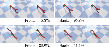
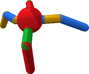
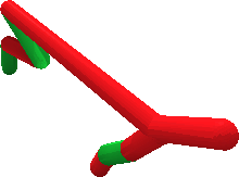
Consider a half-cheetah agent (Fig. 2) trained for locomotion, where the agent must continue walking forward even when one foot is damaged. If we frame this challenge as an RL problem, we must design a reward function that results in a single robustly capable agent. However, prior work \citeprlblogpost,faultyrewards suggests that designing such a reward function is difficult.

As an alternative approach, consider that we have intuition on what behaviors would be useful for adapting to damage. For instance, we can measure how often each foot is used during training, and we can pre-train a collection of policies that are diverse in how the agent uses its feet. When one of the agent’s feet is damaged during deployment, the agent can adapt to the damage by selecting a policy that did not move the damaged foot during training \citepcully2015, colas2020scaling.

Refer to caption — Figure 1: We develop two RL variants of the CMA-MEGA algorithm. Similar to CMA-MEGA, the variants sample gradient coefficients ${\bm{c}}$ and branch around a solution point ${\bm{\phi}}^{*}$ . We evaluate each branched solution ${\bm{\phi}}^{\prime}_{i}$ as part of a policy $\pi_{{\bm{\phi}}^{\prime}_{i}}$ and insert ${\bm{\phi}}^{\prime}_{i}$ into the archive. We then update ${\bm{\phi}}^{*}$ and $\mathcal{N}({\bm{\mu}},{\bm{\Sigma}})$ to maximize archive improvement. Our RL variants differ from CMA-MEGA by approximating gradients with ES and TD3, since exact gradients are unavailable in RL settings.

Pre-training such a collection of policies may be viewed as a quality diversity (QD) optimization problem \citeppugh2016qd,cully2015,mouret2015illuminating, colas2020scaling. Formally, QD assumes an objective function $f$ and one or more measure functions ${\bm{m}}$ . The goal of QD is to find solutions satisfying all output combinations of ${\bm{m}}$ , i.e. moving different combinations of feet, while maximizing each solution’s $f$ , i.e. walking forward quickly. Most QD algorithms treat $f$ and ${\bm{m}}$ as black boxes, but recent work \citepfontaine2021dqd proposes differentiable quality diversity (DQD), which assumes $f$ and ${\bm{m}}$ are differentiable functions with exact gradient information.

The recently proposed DQD algorithm CMA-MEGA \citepfontaine2021dqd outperforms QD algorithms by orders of magnitude when exact gradients are available, such as when searching the latent space of a generative model. However, RL problems like the half-cheetah lack these gradients because the environment is typically non-differentiable, thus limiting the applicability of DQD. To address this limitation, we draw inspiration from how evolution strategies (ES) \citepakimoto2010,wierstra2014nes,salimans2017evolution,mania2018ars and deep RL actor-critic methods \citepschulman2015trpo,schulman2017ppo,lillicrap2016ddpg,fujimoto2018td3 optimize a single objective by approximating gradients for gradient descent. Our key insight is to approximate objective and measure gradients for DQD algorithms by adapting ES and actor-critic methods.

Our work makes three main contributions. (1) We formalize the problem of quality diversity for reinforcement learning (QD-RL) and reduce it to an instance of DQD (Sec. 2). (2) We develop two QD-RL variants of the DQD algorithm CMA-MEGA (Sec. 4). The first variant, CMA-MEGA (ES), approximates objective and measure gradients with ES. The second variant, CMA-MEGA (TD3, ES), approximates the objective gradient with TD3 \citepfujimoto2018td3 (an actor-critic method) and the measure gradients with ES. (3) We benchmark our variants on four PyBullet locomotion tasks from QDGym \citepbenelot2018, qdgym (Sec. 5-6). The first variant, CMA-MEGA (ES), achieves a QD score (Sec. 5.1.3) comparable to the state-of-the-art PGA-MAP-Elites in two tasks. The second variant, CMA-MEGA (TD3, ES), achieves comparable QD score with PGA-MAP-Elites in all tasks but is less efficient than PGA-MAP-Elites in two tasks.

Our results contrast with prior work \citepfontaine2021dqd where CMA-MEGA vastly outperforms OG-MAP-Elites, a DQD algorithm inspired by PGA-MAP-Elites, on benchmark functions where gradient information is available. Overall, we shed light on the limitations of CMA-MEGA in QD domains where the main challenge comes from optimizing the objective rather than from exploring measure space. At the same time, since we decouple gradient estimates from QD optimization, our work opens a path for future research that would benefit from independent improvements to either DQD or RL.

2 Problem Statement

2.1 Quality Diversity (QD)

We adopt the definition of QD from prior work \citepfontaine2021dqd. For a solution vector ${\bm{\phi}}$ , QD considers an objective function $f({\bm{\phi}})$ and $k$ measures¹¹1Prior work has also referred to measures as “behavior characteristics” or “behavior descriptors.” $m_{i}({\bm{\phi}})\in\mathbb{R}$ (for $i\in 1..k$ ) or, as a joint measure, ${\bm{m}}({\bm{\phi}})\in\mathbb{R}^{k}$ . These measures form a $k$ -dimensional measure space $\mathcal{X}$ . For every ${\bm{x}}\in\mathcal{X}$ , the QD objective is to find solution ${\bm{\phi}}$ such that ${\bm{m}}({\bm{\phi}})={\bm{x}}$ and $f({\bm{\phi}})$ is maximized. Since $\mathcal{X}$ is continuous, it would require infinite memory to solve the QD problem, so algorithms in the MAP-Elites family \citepmouret2015illuminating, cully2015 discretize $\mathcal{X}$ by forming a tesselation $\mathcal{Y}$ consisting of $M$ cells. Thus, we relax the QD problem to one of searching for an archive $\mathcal{A}$ consisting of $M$ elites ${\bm{\phi}}_{i}$ , one for each cell in $\mathcal{Y}$ . Then, the QD objective is to maximize the performance $f({\bm{\phi}}_{i})$ of all elites:

\displaystyle\max_{{\bm{\phi}}_{1..M}}\sum_{i=1}^{M}f({\bm{\phi}}_{i})

(1)

2.1.1 Differentiable Quality Diversity (DQD)

In DQD, we assume $f$ and ${\bm{m}}$ are first-order differentiable. We denote the objective gradient as ${\bm{\nabla}}_{f}({\bm{\phi}})$ and the measure gradients as ${\bm{\nabla}}_{\bm{m}}({\bm{\phi}})$ or ${\bm{\nabla}}_{m_{i}}({\bm{\phi}})$ .

2.2 Quality Diversity for Reinforcement Learning (QD-RL)

We define QD-RL as an instance of the QD problem in which the objective $f({\bm{\phi}})$ is the expected discounted return of an RL policy, and the measures ${\bm{m}}({\bm{\phi}})$ are functions of the policy. Formally, drawing on the Markov Decision Process (MDP) formulation \citepSutton2018, we represent QD-RL as a tuple $(\mathcal{S},\mathcal{U},p,r,\gamma,{\bm{m}})$ . On discrete timesteps $t$ in an episode of interaction, an agent observes state $s\in\mathcal{S}$ and takes action $a\in\mathcal{U}$ according to a policy $\pi_{\bm{\phi}}(a|s)$ with parameters ${\bm{\phi}}$ . The agent then receives scalar reward $r(s,a)$ and observes next state $s^{\prime}\in\mathcal{S}$ according to $s^{\prime}\sim p(\cdot|s,a)$ . Each episode thus has a trajectory $\xi=\{s_{0},a_{0},s_{1},a_{1},..,s_{T}\}$ , where $T$ is the number of timesteps in the episode, and the probability that policy $\pi_{\bm{\phi}}$ takes trajectory $\xi$ is $p_{\bm{\phi}}(\xi)=p(s_{0})\prod_{t=0}^{T-1}\pi_{\bm{\phi}}(a_{t}|s_{t})p(s_{t+1}|s_{t},a_{t})$ . Now, we define the expected discounted return of policy $\pi_{\bm{\phi}}$ as

\displaystyle f({\bm{\phi}})=\mathbb{E}_{\xi\sim p_{\bm{\phi}}}\left[\sum_{t=0}^{T}\gamma^{t}r(s_{t},a_{t})\right]

(2)

where the discount factor $\gamma\in(0,1)$ trades off between short- and long-term rewards. Finally, each policy is characterized by a $k$ -dimensional measure function ${\bm{m}}({\bm{\phi}})$ .

2.2.1 QD-RL as an instance of DQD

We reduce QD-RL to a DQD problem. Since the exact gradients ${\bm{\nabla}}_{f}$ and ${\bm{\nabla}}_{\bm{m}}$ usually do not exist in QD-RL, we must instead approximate them.

3 Background

3.1 Single-Objective Reinforcement Learning

We review algorithms which train a policy to maximize a single objective, i.e. $f({\bm{\phi}})$ in Eq. 2, with the goal of applying these algorithms’ gradient approximations to DQD in Sec. 4.

3.1.1 Evolution strategies (ES)

ES \citepbeyer2002 is a class of evolutionary algorithms which optimizes the objective by sampling a population of solutions and moving the population towards areas of higher performance. Natural Evolution Strategies (NES) \citepwierstra2014nes,wierstra2008 is a type of ES which updates the sampling distribution of solutions by taking steps on distribution parameters in the direction of the natural gradient \citepamari1998. For example, with a Gaussian sampling distribution, each iteration of an NES would compute natural gradients to update the mean ${\bm{\mu}}$ and covariance ${\bm{\Sigma}}$ .

We consider two NES-inspired approaches which have demonstrated success in RL domains. First, prior work \citepsalimans2017evolution introduces an algorithm which, drawing from NES, samples $\lambda_{es}$ solutions from an isotropic Gaussian but only computes a gradient step for the mean ${\bm{\phi}}$ . We refer to this algorithm as OpenAI-ES. Each solution sampled by OpenAI-ES is represented as ${\bm{\phi}}+\sigma{\bm{\epsilon}}_{i}$ , where $\sigma$ is the fixed standard deviation of the Gaussian and ${\bm{\epsilon}}_{i}\sim{\mathcal{N}}(\mathbf{0},{\bm{I}})$ . Once these solutions are evaluated, OpenAI-ES estimates the gradient as

\displaystyle{\bm{\nabla}}_{f}({\bm{\phi}})\approx\frac{1}{\lambda_{es}\sigma}\sum_{i=1}^{\lambda_{es}}f({\bm{\phi}}+\sigma{\bm{\epsilon}}_{i}){\bm{\epsilon}}_{i}

(3)

OpenAI-ES then passes this estimate to an Adam optimizer \citepadam which outputs a gradient ascent step for ${\bm{\phi}}$ . To make the estimate more accurate, OpenAI-ES further includes techniques such as mirror sampling and rank normalization \citepha2017visual,wierstra2014nes.

3.1.2 Actor-critic methods

While ES treats the objective as a black box, actor-critic methods leverage the MDP structure of the objective, i.e. the fact that $f({\bm{\phi}})$ is a sum of Markovian values. We are most interested in Twin Delayed Deep Deterministic policy gradient (TD3) \citepfujimoto2018td3, an off-policy actor-critic method. TD3 maintains (1) an actor consisting of the policy $\pi_{\bm{\phi}}$ and (2) a critic consisting of state-action value functions $Q_{{\bm{\theta}}_{1}}(s,a)$ and $Q_{{\bm{\theta}}_{2}}(s,a)$ which differ only in random initialization. Through interactions in the environment, the actor generates experience which is stored in a replay buffer $\mathcal{B}$ . This experience is sampled to train $Q_{{\bm{\theta}}_{1}}$ and $Q_{{\bm{\theta}}_{2}}$ . Simultaneously, the actor improves by maximizing $Q_{{\bm{\theta}}_{1}}$ via gradient ascent ( $Q_{{\bm{\theta}}_{2}}$ is only used during critic training). Specifically, for an objective $f^{\prime}$ which is based on the critic and approximates $f$ , TD3 estimates a gradient ${\bm{\nabla}}_{f^{\prime}}({\bm{\phi}})$ and passes it to an Adam optimizer. Notably, TD3 never updates network weights directly, instead accumulating weights into target networks $\pi_{{\bm{\phi}}^{\prime}}$ , $Q_{{\bm{\theta}}^{\prime}_{1}}$ , $Q_{{\bm{\theta}}^{\prime}_{2}}$ via an exponentially weighted moving average with update rate $\tau$ .

3.2 Quality Diversity Algorithms

3.2.1 MAP-Elites extensions for QD-RL

One of the simplest QD algorithms is MAP-Elites \citepmouret2015illuminating, cully2015. MAP-Elites creates an archive $\mathcal{A}$ by tesselating the measure space $\mathcal{X}$ into a grid of evenly-sized cells. Then, it draws $\lambda$ initial solutions from a multivariate Gaussian $\mathcal{N}(\mathbf{{\bm{\phi}}_{0}},\sigma{\bm{I}})$ centered at some ${\bm{\phi}}_{0}$ . Next, for each sampled solution ${\bm{\phi}}$ , MAP-Elites computes $f({\bm{\phi}})$ and ${\bm{m}}({\bm{\phi}})$ and inserts ${\bm{\phi}}$ into $\mathcal{A}$ . In subsequent iterations, MAP-Elites randomly selects $\lambda$ solutions from $\mathcal{A}$ and adds Gaussian noise, i.e. solution ${\bm{\phi}}$ becomes ${\bm{\phi}}+\mathcal{N}(\mathbf{0},\sigma{\bm{I}})$ . Solutions are placed into cells based on their measures; if a solution has higher $f$ than the solution currently in the cell, it replaces that solution. Once inserted into $\mathcal{A}$ , solutions are known as elites.

Due to the high dimensionality of neural network parameters, MAP-Elites has not proven effective for QD-RL. Hence, several extensions merge MAP-Elites with actor-critic methods and ES. For instance, Policy Gradient Assisted MAP-Elites (PGA-MAP-Elites) \citepnilsson2021pga combines MAP-Elites with TD3. Each iteration, PGA-MAP-Elites evaluates $\lambda$ solutions for insertion into the archive. $\frac{\lambda}{2}$ of these are created by selecting random solutions from the archive and taking gradient ascent steps with a TD3 critic. The other $\frac{\lambda}{2}$ solutions are created with a directional variation operator \citepvassiliades2018line which selects two solutions ${\bm{\phi}}_{1}$ and ${\bm{\phi}}_{2}$ from the archive and creates a new one according to ${\bm{\phi}}^{\prime}={\bm{\phi}}_{1}+\sigma_{1}\mathcal{N}(\mathbf{0},{\bm{I}})+\sigma_{2}({\bm{\phi}}_{2}-{\bm{\phi}}_{1})\mathcal{N}(0,1)$ . PGA-MAP-Elites achieves state-of-the-art performance on locomotion tasks in the QDGym benchmark \citepqdgym.

Another MAP-Elites extension is ME-ES \citepcolas2020scaling, which combines MAP-Elites with an OpenAI-ES optimizer. In the “explore-exploit” variant, ME-ES alternates between two phases. In the “exploit” phase, ME-ES restarts OpenAI-ES at a mean ${\bm{\phi}}$ and optimizes the objective for $k$ iterations, inserting the current ${\bm{\phi}}$ into the archive in each iteration. In the “explore” phase, ME-ES repeats this process, but OpenAI-ES instead optimizes for novelty, where novelty is the distance in measure space from a new solution to previously encountered solutions. ME-ES also has an “exploit” variant and an “explore” variant, which each execute only one type of phase.

Our work is related to ME-ES in that we also adapt OpenAI-ES, but instead of alternating between following a novelty gradient and objective gradient, we compute all objective and measure gradients and allow a CMA-ES \citephansen2016tutorial instance to decide which gradients to follow to maximize QD score. We include MAP-Elites, PGA-MAP-Elites, and ME-ES as baselines in our experiments.

3.2.2 Covariance Matrix Adaptation MAP-Elites via a Gradient Arborescence (CMA-MEGA)

We directly extend CMA-MEGA \citepfontaine2021dqd to address QD-RL. CMA-MEGA is a DQD algorithm based on the QD algorithm CMA-ME \citepfontaine2020covariance. The intuition behind CMA-MEGA is that for solution ${\bm{\phi}}$ , we can simultaneously increase/decrease both the objective and measures by following the objective and measure gradients of ${\bm{\phi}}$ . In doing so, we traverse objective-measure space and generate solutions which maximize improvement of the archive.

Each iteration, CMA-MEGA first calculates objective and measure gradients for a mean solution ${\bm{\phi}}^{*}$ . Next, it generates $\lambda$ new solutions by sampling gradient coefficients ${\bm{c}}\sim\mathcal{N}({\bm{\mu}},{\bm{\Sigma}})$ and computing ${\bm{\phi}}^{\prime}\leftarrow{\bm{\phi}}^{*}+{\bm{c}}_{0}{\bm{\nabla}}_{f}({\bm{\phi}}^{*})+\sum_{j=1}^{k}{\bm{c}}_{j}{\bm{\nabla}}_{m_{j}}({\bm{\phi}}^{*})$ . CMA-MEGA inserts these solutions into the archive and computes their improvement, $\Delta$ . $\Delta$ is defined as $f({\bm{\phi}}^{\prime})$ if ${\bm{\phi}}^{\prime}$ populates a new cell, and $f({\bm{\phi}}^{\prime})-f({\bm{\phi}}^{\prime}_{\mathcal{E}})$ if ${\bm{\phi}}^{\prime}$ improves an existing cell (replaces a previous solution ${\bm{\phi}}^{\prime}_{\mathcal{E}}$ ). After CMA-MEGA inserts the solutions, it ranks them by $\Delta$ . If a solution populates a new cell, its $\Delta$ always ranks higher than that of a solution which only improves an existing cell. Finally, CMA-MEGA passes the ranking to CMA-ES \citephansen2016tutorial, which adapts ${\bm{\mu}}$ and ${\bm{\Sigma}}$ such that future gradient coefficients ${\bm{c}}$ are more likely to generate archive improvement. By leveraging gradient information, CMA-MEGA solves QD benchmarks with orders of magnitude fewer solution evaluations than previous QD algorithms.

4 Approximating Gradients for CMA-MEGA

Since CMA-MEGA requires exact objective and measure gradients, we cannot directly apply it to QD-RL. To address this limitation, we replace exact gradients with gradient approximations (Sec. 4.1) and develop two CMA-MEGA variants (Sec. 4.2).

4.1 Approximating Objective and Measure Gradients

We adapt gradient approximations from ES and actor-critic methods. Since the objective has an MDP structure, we estimate objective gradients ${\bm{\nabla}}_{f}$ with ES and actor-critic methods. Since the measures are black boxes, we estimate measure gradients ${\bm{\nabla}}_{\bm{m}}$ with ES.

4.1.1 Approximating objective gradients with ES and actor-critic methods

We estimate objective gradients with two methods. First, we treat the objective as a black box and estimate its gradient with a black box method, i.e. the OpenAI-ES gradient estimate in Eq. 3. Since OpenAI-ES performs well in RL domains \citepsalimans2017evolution,pagliuca2020,lehman2018, we believe this estimate is suitable for approximating gradients for CMA-MEGA in QD-RL settings. Importantly, this estimate requires environment interaction by evaluating $\lambda_{es}$ solutions.

Since the objective has a well-defined structure, i.e. it is a sum of rewards from an MDP (Eq. 2), we also estimate its gradient with an actor-critic method, TD3. TD3 is well-suited for this purpose because it efficiently estimates objective gradients for the multiple policies that CMA-MEGA and other QD-RL algorithms generate. In particular, once the critic is trained, TD3 can provide a gradient estimate for any policy without additional environment interaction.

Among actor-critic methods, we select TD3 since it achieves high performance while optimizing primarily for the RL objective. Prior work \citepfujimoto2018td3 shows that TD3 outperforms on-policy methods \citepschulman2015trpo,schulman2017ppo. While the off-policy Soft Actor-Critic \citephaarnoja2018sac algorithm can outperform TD3, it optimizes a maximum-entropy objective designed to encourage exploration. In our work, this exploration is unnecessary because QD algorithms already search for diverse solutions.

4.1.2 Approximating measure gradients with ES

Since we treat measures as black boxes (Sec. 2.2), we can only estimate their gradient with black box methods. Thus, similar to the objective, we approximate each individual measure’s gradient ${\bm{\nabla}}_{m_{i}}$ with the OpenAI-ES gradient estimate, replacing $f$ with $m_{i}$ in Eq. 3.

Since the OpenAI-ES gradient estimate requires additional environment interaction, all of our CMA-MEGA variants require environment interaction to estimate gradients. However, the environment interaction required to estimate measure gradients remains constant even as the number of measures increases, since we can reuse the same $\lambda_{es}$ solutions to estimate each ${\bm{\nabla}}_{m_{i}}$ .

In problems where the measures have an MDP structure similar to the objective, it may be feasible to estimate each ${\bm{\nabla}}_{m_{i}}$ with its own TD3 instance. In the environments in our work (Sec. 5.1), each measure is non-Markovian since it calculates the proportion of time a walking agent’s foot spends on the ground. This calculation depends on the entire agent trajectory rather than on one state.

4.2 CMA-MEGA Variants

Our choice of gradient approximations leads to two CMA-MEGA variants. CMA-MEGA (ES) approximates objective and measure gradients with OpenAI-ES, while CMA-MEGA (TD3, ES) approximates the objective gradient with TD3 and the measure gradients with OpenAI-ES. Refer to Appendix B for a detailed explanation of these algorithms.

5 Experiments

We compare our two proposed CMA-MEGA variants (CMA-MEGA (ES), CMA-MEGA (TD3, ES)) with three baselines (PGA-MAP-Elites, ME-ES, MAP-Elites) in four locomotion tasks. We implement MAP-Elites as described in Sec. 3.2.1, and we select the explore-exploit variant for ME-ES since it has performed at least as well as both the explore variant and the exploit variant in several domains \citepcolas2020scaling.

5.1 Evaluation Domains

5.1.1 QDGym

We evaluate our algorithms in four locomotion environments from QDGym \citepqdgym, a library built on PyBullet Gym \citepcoumans2020, benelot2018 and OpenAI Gym \citepbrockman2016gym. Table LABEL:table:envs, Appendix D lists all environment details. In each environment, the QD algorithm outputs an archive of walking policies for a simulated agent. The agent is primarily rewarded for its forward speed. There are also reward shaping \citepng1999shaping signals, such as a punishment for applying higher joint torques, intended to guide policy optimization. The measures compute the proportion of time (number of timesteps divided by total timesteps in an episode) that each of the agent’s feet contacts the ground.

QDGym is challenging because the objective in each environment does not “align” with the measures, in that finding policies with different measures (i.e. exploring the archive) does not necessarily lead to optimization of the objective. While it may be trivial to fill the archive with low-performing policies which stand in place and lift the feet up and down to achieve different measures, the agents’ complexity (high degrees of freedom) makes it difficult to learn a high-performing policy for each value of the measures.

5.1.2 Hyperparameters

Each agent’s policy is a neural network which takes in states and outputs actions. There are two hidden layers of 128 nodes, and the hidden and output layers have tanh activation. We initialize weights with Xavier initialization \citepglorot2010. For the archive, we tesselate each environment’s measure space into a grid of evenly-sized cells (see Table LABEL:table:envs for grid dimensions). Each measure is bound to the range $[0,1]$ , the min and max proportion of time that one foot can contact the ground. Each algorithm evaluates 1 million solutions in the environment. Due to computational limits, we evaluate each solution once instead of averaging multiple episodes, so each algorithm runs 1 million episodes total. Refer to Appendix C for further hyperparameters.

5.1.3 Metrics

Our primary metric is QD score \citeppugh2016qd, which provides a holistic view of algorithm performance. QD score is the sum of the objective values of all elites in the archive, i.e. $\sum_{i=1}^{M}\bm{1}_{{\bm{\phi}}_{i}\mathrm{exists}}f({\bm{\phi}}_{i})$ , where $M$ is the number of archive cells. We set the objective $f$ to be the expected undiscounted return, i.e. we set $\gamma=1$ in Eq. 2.

Since objectives may be negative, an algorithm’s QD score may be penalized when adding a new solution. To prevent this, we define a minimum objective in each environment by taking the lowest objective value that was inserted into the archive in any experiment in that environment. We subtract this minimum from every solution, such that every solution that was inserted into an archive has an objective value of at least 0. Thus, we use QD score defined as $\sum_{i=1}^{M}\bm{1}_{{\bm{\phi}}_{i}\mathrm{exists}}(f({\bm{\phi}}_{i})-\mathrm{min\ objective})$ . We also define a maximum objective equivalent to each environment’s “reward threshold” in PyBullet Gym. This threshold is the objective value at which an agent is considered to have successfully learned to walk.

We report two metrics in addition to QD score. Archive coverage, the proportion of cells for which the algorithm found an elite, gauges how well the QD algorithm explores measure space, and best performance, the highest objective of any elite in the archive, gauges how well the QD algorithm exploits the objective.

5.2 Experimental Design

We follow a between-groups design, where the two independent variables are environment (QD Ant, QD Half-Cheetah, QD Hopper, QD Walker) and algorithm (CMA-MEGA (ES), CMA-MEGA (TD3, ES), PGA-MAP-Elites, ME-ES, MAP-Elites). The dependent variable is the QD score. In each environment, we run each algorithm for 5 trials with different random seeds. We test three hypotheses: [H1] In each environment, CMA-MEGA (ES) will outperform (with respect to QD score) all baselines (PGA-MAP-Elites, ME-ES, MAP-Elites). [H2] In each environment, CMA-MEGA (TD3, ES) will outperform all baselines. [H3] In each environment, CMA-MEGA (TD3, ES) will outperform CMA-MEGA (ES).

H1 and H2 are based on prior work \citepfontaine2021dqd which showed that in QD benchmark domains, CMA-MEGA outperforms algorithms that do not leverage both objective and measure gradients. H3 is based on results \citeppagliuca2020 which suggest that actor-critic methods outperform ES in PyBullet Gym. Thus, we expect the TD3 objective gradient to be more accurate than the ES objective gradient, leading to more efficient traversal of objective-measure space and higher QD score.

5.3 Implementation

We implement all QD algorithms with the pyribs library \citeppyribs except for ME-ES, which we adapt from the authors’ implementation. We run each experiment with 100 CPUs on a high-performance cluster. We allocate one NVIDIA Tesla P100 GPU to algorithms that train TD3 (CMA-MEGA (TD3, ES) and PGA-MAP-Elites). Depending on the algorithm and environment, each experiment lasts 4-20 hours; refer to Table 11, Appendix E for mean runtimes.

6 Results

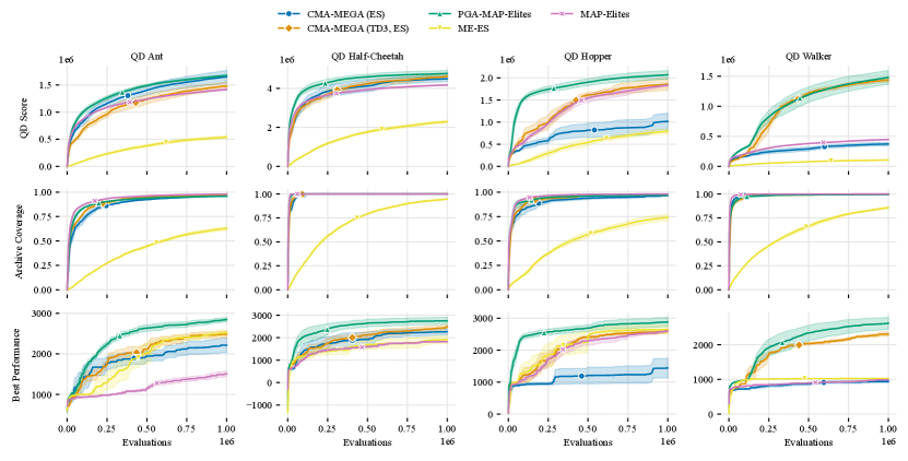
We ran 5 trials of each algorithm in each environment. In each trial, we allocated 1 million evaluations and recorded the QD score, archive coverage, and best performance. Fig. 3 plots the metrics from our experiments, and Appendix E lists final values of all metrics. Appendix H shows example heatmaps and histograms of each archive, and the supplemental material contains videos of generated agents. Refer to Appendix G for a discussion of our results.

7 Conclusion

To extend DQD to RL settings, we adapted gradient approximations from actor-critic methods and ES. By integrating these approximations with CMA-MEGA, we proposed two novel variants that we evaluated on four locomotion tasks from QDGym. CMA-MEGA (TD3, ES) performed comparably to the state-of-the-art PGA-MAP-Elites in all tasks but was less efficient in two of the tasks. CMA-MEGA (ES) performed comparably in two tasks. Since we decouple DQD from gradient approximations, our work opens avenues for future research which expands the applicability of DQD in RL settings, by independently developing either more accurate gradient approximations or more powerful DQD algorithms.

References

[1]
[\citeauthoryearAkimoto, Nagata, Ono, and KobayashiAkimoto et al.2010] Youhei Akimoto, Yuichi Nagata, Isao Ono, and Shigenobu Kobayashi. 2010. Bidirectional Relation between CMA Evolution Strategies and Natural Evolution Strategies. In Parallel Problem Solving from Nature, PPSN XI, Robert Schaefer, Carlos Cotta, Joanna Kołodziej, and Günter Rudolph (Eds.). Springer Berlin Heidelberg, Berlin, Heidelberg, 154–163.
[\citeauthoryearAmariAmari1998] Shun-ichi Amari. 1998. Natural Gradient Works Efficiently in Learning. Neural Computation 10, 2 (02 1998), 251–276. https://doi.org/10.1162/089976698300017746 arXiv:https://direct.mit.edu/neco/article-pdf/10/2/251/813415/089976698300017746.pdf
[\citeauthoryearAndrychowicz, Wolski, Ray, Schneider, Fong, Welinder, McGrew, Tobin, Pieter Abbeel, and ZarembaAndrychowicz et al.2017] Marcin Andrychowicz, Filip Wolski, Alex Ray, Jonas Schneider, Rachel Fong, Peter Welinder, Bob McGrew, Josh Tobin, OpenAI Pieter Abbeel, and Wojciech Zaremba. 2017. Hindsight Experience Replay. In Advances in Neural Information Processing Systems, I. Guyon, U. V. Luxburg, S. Bengio, H. Wallach, R. Fergus, S. Vishwanathan, and R. Garnett (Eds.), Vol. 30. Curran Associates, Inc. https://proceedings.neurips.cc/paper/2017/file/453fadbd8a1a3af50a9df4df899537b5-Paper.pdf
[\citeauthoryearBeyer and SchwefelBeyer and Schwefel2002] Hans-Georg Beyer and Hans-Paul Schwefel. 2002. Evolution strategies – A comprehensive introduction. Natural Computing 1, 1 (01 Mar 2002), 3–52. https://doi.org/10.1023/A:1015059928466
[\citeauthoryearBrockman, Cheung, Pettersson, Schneider, Schulman, Tang, and ZarembaBrockman et al.2016] Greg Brockman, Vicki Cheung, Ludwig Pettersson, Jonas Schneider, John Schulman, Jie Tang, and Wojciech Zaremba. 2016. OpenAI Gym. CoRR abs/1606.01540 (2016). arXiv:1606.01540 http://arxiv.org/abs/1606.01540
[\citeauthoryearCideron, Pierrot, Perrin, Beguir, and SigaudCideron et al.2020] Geoffrey Cideron, Thomas Pierrot, Nicolas Perrin, Karim Beguir, and Olivier Sigaud. 2020. QD-RL: Efficient Mixing of Quality and Diversity in Reinforcement Learning. CoRR abs/2006.08505 (2020). arXiv:2006.08505 https://arxiv.org/abs/2006.08505
[\citeauthoryearClark and AmodeiClark and Amodei2016] Jack Clark and Dario Amodei. 2016. Faulty Reward Functions in the Wild. https://openai.com/blog/faulty-reward-functions/.
[\citeauthoryearColas, Madhavan, Huizinga, and CluneColas et al.2020] Cédric Colas, Vashisht Madhavan, Joost Huizinga, and Jeff Clune. 2020. Scaling MAP-Elites to Deep Neuroevolution. In Proceedings of the 2020 Genetic and Evolutionary Computation Conference (Cancún, Mexico) (GECCO ’20). Association for Computing Machinery, New York, NY, USA, 67–75. https://doi.org/10.1145/3377930.3390217
[\citeauthoryearColas, Sigaud, and OudeyerColas et al.2018] Cédric Colas, Olivier Sigaud, and Pierre-Yves Oudeyer. 2018. GEP-PG: Decoupling Exploration and Exploitation in Deep Reinforcement Learning Algorithms. In Proceedings of the 35th International Conference on Machine Learning (Proceedings of Machine Learning Research, Vol. 80), Jennifer Dy and Andreas Krause (Eds.). PMLR, 1039–1048. https://proceedings.mlr.press/v80/colas18a.html
[\citeauthoryearConti, Madhavan, Petroski Such, Lehman, Stanley, and CluneConti et al.2018] Edoardo Conti, Vashisht Madhavan, Felipe Petroski Such, Joel Lehman, Kenneth Stanley, and Jeff Clune. 2018. Improving Exploration in Evolution Strategies for Deep Reinforcement Learning via a Population of Novelty-Seeking Agents. In Advances in Neural Information Processing Systems 31, S. Bengio, H. Wallach, H. Larochelle, K. Grauman, N. Cesa-Bianchi, and R. Garnett (Eds.). Curran Associates, Inc., 5027–5038. http://papers.nips.cc/paper/7750-improving-exploration-in-evolution-strategies-for-deep-reinforcement-learning-via-a-population-of-novelty-seeking-agents.pdf
[\citeauthoryearCoumans and BaiCoumans and Bai2020] Erwin Coumans and Yunfei Bai. 2016–2020. PyBullet, a Python module for physics simulation for games, robotics and machine learning. http://pybullet.org.
[\citeauthoryearCully, Clune, Tarapore, and MouretCully et al.2015] Antoine Cully, Jeff Clune, Danesh Tarapore, and Jean-Baptiste Mouret. 2015. Robots that can adapt like animals. Nature 521 (05 2015), 503–507. https://doi.org/10.1038/nature14422
[\citeauthoryearde Boer, Kroese, Mannor, and Rubinsteinde Boer et al.2005] Pieter-Tjerk de Boer, Dirk P. Kroese, Shie Mannor, and Reuven Y. Rubinstein. 2005. A Tutorial on the Cross-Entropy Method. Annals of Operations Research 134, 1 (01 Feb 2005), 19–67. https://doi.org/10.1007/s10479-005-5724-z
[\citeauthoryearEllenbergerEllenberger2019] Benjamin Ellenberger. 2018–2019. PyBullet Gymperium. https://github.com/benelot/pybullet-gym.
[\citeauthoryearEysenbach, Gupta, Ibarz, and LevineEysenbach et al.2019] Benjamin Eysenbach, Abhishek Gupta, Julian Ibarz, and Sergey Levine. 2019. Diversity is All You Need: Learning Skills without a Reward Function. In International Conference on Learning Representations. https://openreview.net/forum?id=SJx63jRqFm
[\citeauthoryearFontaine and NikolaidisFontaine and Nikolaidis2021] Matthew C. Fontaine and Stefanos Nikolaidis. 2021. Differentiable Quality Diversity. Advances in Neural Information Processing Systems 34 (2021). https://proceedings.neurips.cc/paper/2021/file/532923f11ac97d3e7cb0130315b067dc-Paper.pdf
[\citeauthoryearFontaine, Togelius, Nikolaidis, and HooverFontaine et al.2020] Matthew C. Fontaine, Julian Togelius, Stefanos Nikolaidis, and Amy K. Hoover. 2020. Covariance Matrix Adaptation for the Rapid Illumination of Behavior Space. In Proceedings of the 2020 Genetic and Evolutionary Computation Conference (Cancún, Mexico) (GECCO ’20). Association for Computing Machinery, New York, NY, USA, 94–102. https://doi.org/10.1145/3377930.3390232
[\citeauthoryearFujimoto, van Hoof, and MegerFujimoto et al.2018] Scott Fujimoto, Herke van Hoof, and David Meger. 2018. Addressing Function Approximation Error in Actor-Critic Methods. In Proceedings of the 35th International Conference on Machine Learning (Proceedings of Machine Learning Research, Vol. 80), Jennifer Dy and Andreas Krause (Eds.). PMLR, 1587–1596. http://proceedings.mlr.press/v80/fujimoto18a.html
[\citeauthoryearGlorot and BengioGlorot and Bengio2010] Xavier Glorot and Yoshua Bengio. 2010. Understanding the difficulty of training deep feedforward neural networks. In Proceedings of the Thirteenth International Conference on Artificial Intelligence and Statistics (Proceedings of Machine Learning Research, Vol. 9), Yee Whye Teh and Mike Titterington (Eds.). PMLR, Chia Laguna Resort, Sardinia, Italy, 249–256. https://proceedings.mlr.press/v9/glorot10a.html
[\citeauthoryearHaHa2017] David Ha. 2017. A Visual Guide to Evolution Strategies. blog.otoro.net (2017). https://blog.otoro.net/2017/10/29/visual-evolution-strategies/
[\citeauthoryearHaarnoja, Zhou, Abbeel, and LevineHaarnoja et al.2018] Tuomas Haarnoja, Aurick Zhou, Pieter Abbeel, and Sergey Levine. 2018. Soft Actor-Critic: Off-Policy Maximum Entropy Deep Reinforcement Learning with a Stochastic Actor. In Proceedings of the 35th International Conference on Machine Learning (Proceedings of Machine Learning Research, Vol. 80), Jennifer Dy and Andreas Krause (Eds.). PMLR, 1861–1870. https://proceedings.mlr.press/v80/haarnoja18b.html
[\citeauthoryearHansenHansen2016] Nikolaus Hansen. 2016. The CMA Evolution Strategy: A Tutorial. CoRR abs/1604.00772 (2016). arXiv:1604.00772 http://arxiv.org/abs/1604.00772
[\citeauthoryearIrpanIrpan2018] Alex Irpan. 2018. Deep Reinforcement Learning Doesn’t Work Yet. https://www.alexirpan.com/2018/02/14/rl-hard.html.
[\citeauthoryearKhadka, Majumdar, Nassar, Dwiel, Tumer, Miret, Liu, and TumerKhadka et al.2019] Shauharda Khadka, Somdeb Majumdar, Tarek Nassar, Zach Dwiel, Evren Tumer, Santiago Miret, Yinyin Liu, and Kagan Tumer. 2019. Collaborative Evolutionary Reinforcement Learning. In Proceedings of the 36th International Conference on Machine Learning (Proceedings of Machine Learning Research, Vol. 97), Kamalika Chaudhuri and Ruslan Salakhutdinov (Eds.). PMLR, 3341–3350. https://proceedings.mlr.press/v97/khadka19a.html
[\citeauthoryearKhadka and TumerKhadka and Tumer2018] Shauharda Khadka and Kagan Tumer. 2018. Evolution-Guided Policy Gradient in Reinforcement Learning. In Advances in Neural Information Processing Systems, S. Bengio, H. Wallach, H. Larochelle, K. Grauman, N. Cesa-Bianchi, and R. Garnett (Eds.), Vol. 31. Curran Associates, Inc. https://proceedings.neurips.cc/paper/2018/file/85fc37b18c57097425b52fc7afbb6969-Paper.pdf
[\citeauthoryearKingma and BaKingma and Ba2015] Diederik P. Kingma and Jimmy Ba. 2015. Adam: A Method for Stochastic Optimization. In 3rd International Conference on Learning Representations, ICLR 2015, San Diego, CA, USA, May 7-9, 2015, Conference Track Proceedings, Yoshua Bengio and Yann LeCun (Eds.). http://arxiv.org/abs/1412.6980
[\citeauthoryearKumar, Kumar, Levine, and FinnKumar et al.2020] Saurabh Kumar, Aviral Kumar, Sergey Levine, and Chelsea Finn. 2020. One Solution is Not All You Need: Few-Shot Extrapolation via Structured MaxEnt RL. Advances in Neural Information Processing Systems 33 (2020).
[\citeauthoryearLehman, Chen, Clune, and StanleyLehman et al.2018] Joel Lehman, Jay Chen, Jeff Clune, and Kenneth O. Stanley. 2018. ES is More than Just a Traditional Finite-Difference Approximator. In Proceedings of the Genetic and Evolutionary Computation Conference (Kyoto, Japan) (GECCO ’18). Association for Computing Machinery, New York, NY, USA, 450–457. https://doi.org/10.1145/3205455.3205474
[\citeauthoryearLehman and StanleyLehman and Stanley2011a] Joel Lehman and Kenneth O. Stanley. 2011a. Abandoning Objectives: Evolution Through the Search for Novelty Alone. Evolutionary Computation 19, 2 (06 2011), 189–223. https://doi.org/10.1162/EVCO_a_00025 arXiv:https://direct.mit.edu/evco/article-pdf/19/2/189/1494066/evco_a_00025.pdf
[\citeauthoryearLehman and StanleyLehman and Stanley2011b] Joel Lehman and Kenneth O. Stanley. 2011b. Evolving a Diversity of Virtual Creatures through Novelty Search and Local Competition. In Proceedings of the 13th Annual Conference on Genetic and Evolutionary Computation (Dublin, Ireland) (GECCO ’11). Association for Computing Machinery, New York, NY, USA, 211–218. https://doi.org/10.1145/2001576.2001606
[\citeauthoryearLi, Song, and ErmonLi et al.2017] Yunzhu Li, Jiaming Song, and Stefano Ermon. 2017. InfoGAIL: Interpretable Imitation Learning from Visual Demonstrations. In Advances in Neural Information Processing Systems, I. Guyon, U. V. Luxburg, S. Bengio, H. Wallach, R. Fergus, S. Vishwanathan, and R. Garnett (Eds.), Vol. 30. Curran Associates, Inc. https://proceedings.neurips.cc/paper/2017/file/2cd4e8a2ce081c3d7c32c3cde4312ef7-Paper.pdf
[\citeauthoryearLillicrap, Hunt, Pritzel, Heess, Erez, Tassa, Silver, and WierstraLillicrap et al.2016] Timothy P. Lillicrap, Jonathan J. Hunt, Alexander Pritzel, Nicolas Heess, Tom Erez, Yuval Tassa, David Silver, and Daan Wierstra. 2016. Continuous control with deep reinforcement learning. In 4th International Conference on Learning Representations, ICLR 2016, San Juan, Puerto Rico, May 2-4, 2016, Conference Track Proceedings, Yoshua Bengio and Yann LeCun (Eds.). http://arxiv.org/abs/1509.02971
[\citeauthoryearMania, Guy, and RechtMania et al.2018] Horia Mania, Aurelia Guy, and Benjamin Recht. 2018. Simple Random Search of Static Linear Policies is Competitive for Reinforcement Learning. In Proceedings of the 32nd International Conference on Neural Information Processing Systems (Montréal, Canada) (NIPS’18). Curran Associates Inc., Red Hook, NY, USA, 1805–1814.
[\citeauthoryearMouret and CluneMouret and Clune2015] Jean-Baptiste Mouret and Jeff Clune. 2015. Illuminating search spaces by mapping elites. CoRR abs/1504.04909 (2015). arXiv:1504.04909 http://arxiv.org/abs/1504.04909
[\citeauthoryearNg, Harada, and RussellNg et al.1999] Andrew Y. Ng, Daishi Harada, and Stuart J. Russell. 1999. Policy Invariance Under Reward Transformations: Theory and Application to Reward Shaping. In Proceedings of the Sixteenth International Conference on Machine Learning (ICML ’99). Morgan Kaufmann Publishers Inc., San Francisco, CA, USA, 278–287.
[\citeauthoryearNilssonNilsson2021] Olle Nilsson. 2021. QDgym. https://github.com/ollenilsson19/QDgym.
[\citeauthoryearNilsson and CullyNilsson and Cully2021] Olle Nilsson and Antoine Cully. 2021. Policy Gradient Assisted MAP-Elites. In Proceedings of the Genetic and Evolutionary Computation Conference (Lille, France) (GECCO ’21). Association for Computing Machinery, New York, NY, USA, 866–875. https://doi.org/10.1145/3449639.3459304
[\citeauthoryearPagliuca, Milano, and NolfiPagliuca et al.2020] Paolo Pagliuca, Nicola Milano, and Stefano Nolfi. 2020. Efficacy of Modern Neuro-Evolutionary Strategies for Continuous Control Optimization. Frontiers in Robotics and AI 7 (2020), 98. https://doi.org/10.3389/frobt.2020.00098
[\citeauthoryearParker-Holder, Pacchiano, Choromanski, and RobertsParker-Holder et al.2020] Jack Parker-Holder, Aldo Pacchiano, Krzysztof M Choromanski, and Stephen J Roberts. 2020. Effective Diversity in Population Based Reinforcement Learning. In Advances in Neural Information Processing Systems, H. Larochelle, M. Ranzato, R. Hadsell, M. F. Balcan, and H. Lin (Eds.), Vol. 33. Curran Associates, Inc., 18050–18062. https://proceedings.neurips.cc/paper/2020/file/d1dc3a8270a6f9394f88847d7f0050cf-Paper.pdf
[\citeauthoryearPourchot and SigaudPourchot and Sigaud2019] Pourchot and Sigaud. 2019. CEM-RL: Combining evolutionary and gradient-based methods for policy search. In International Conference on Learning Representations. https://openreview.net/forum?id=BkeU5j0ctQ
[\citeauthoryearPugh, Soros, and StanleyPugh et al.2016] Justin K. Pugh, Lisa B. Soros, and Kenneth O. Stanley. 2016. Quality Diversity: A New Frontier for Evolutionary Computation. Frontiers in Robotics and AI 3 (2016), 40. https://doi.org/10.3389/frobt.2016.00040
[\citeauthoryearSalimans, Ho, Chen, Sidor, and SutskeverSalimans et al.2017] Tim Salimans, Jonathan Ho, Xi Chen, Szymon Sidor, and Ilya Sutskever. 2017. Evolution Strategies as a Scalable Alternative to Reinforcement Learning. arXiv:1703.03864 [stat.ML]
[\citeauthoryearSchaul, Horgan, Gregor, and SilverSchaul et al.2015] Tom Schaul, Daniel Horgan, Karol Gregor, and David Silver. 2015. Universal Value Function Approximators. In Proceedings of the 32nd International Conference on Machine Learning (Proceedings of Machine Learning Research, Vol. 37), Francis Bach and David Blei (Eds.). PMLR, Lille, France, 1312–1320. https://proceedings.mlr.press/v37/schaul15.html
[\citeauthoryearSchulman, Levine, Abbeel, Jordan, and MoritzSchulman et al.2015] John Schulman, Sergey Levine, Pieter Abbeel, Michael Jordan, and Philipp Moritz. 2015. Trust Region Policy Optimization. In Proceedings of the 32nd International Conference on Machine Learning (Proceedings of Machine Learning Research, Vol. 37), Francis Bach and David Blei (Eds.). PMLR, Lille, France, 1889–1897. https://proceedings.mlr.press/v37/schulman15.html
[\citeauthoryearSchulman, Wolski, Dhariwal, Radford, and KlimovSchulman et al.2017] John Schulman, Filip Wolski, Prafulla Dhariwal, Alec Radford, and Oleg Klimov. 2017. Proximal Policy Optimization Algorithms. CoRR abs/1707.06347 (2017). arXiv:1707.06347 http://arxiv.org/abs/1707.06347
[\citeauthoryearSutton and BartoSutton and Barto2018] Richard S. Sutton and Andrew G. Barto. 2018. Reinforcement Learning: An Introduction (second ed.). The MIT Press. http://incompleteideas.net/book/the-book-2nd.html
[\citeauthoryearTangTang2021] Yunhao Tang. 2021. Guiding Evolutionary Strategies with Off-Policy Actor-Critic. In Proceedings of the 20th International Conference on Autonomous Agents and MultiAgent Systems (Virtual Event, United Kingdom) (AAMAS ’21). International Foundation for Autonomous Agents and Multiagent Systems, Richland, SC, 1317–1325.
[\citeauthoryearTjanaka, Fontaine, Zhang, Sommerer, Dennler, and NikolaidisTjanaka et al.2021] Bryon Tjanaka, Matthew C. Fontaine, Yulun Zhang, Sam Sommerer, Nathan Dennler, and Stefanos Nikolaidis. 2021. pyribs: A bare-bones Python library for quality diversity optimization. https://github.com/icaros-usc/pyribs.
[\citeauthoryearVassiliades and MouretVassiliades and Mouret2018] Vassilis Vassiliades and Jean-Baptiste Mouret. 2018. Discovering the Elite Hypervolume by Leveraging Interspecies Correlation. In Proceedings of the Genetic and Evolutionary Computation Conference (Kyoto, Japan) (GECCO ’18). Association for Computing Machinery, New York, NY, USA, 149–156. https://doi.org/10.1145/3205455.3205602
[\citeauthoryearWierstra, Schaul, Glasmachers, Sun, Peters, and SchmidhuberWierstra et al.2014] Daan Wierstra, Tom Schaul, Tobias Glasmachers, Yi Sun, Jan Peters, and Jürgen Schmidhuber. 2014. Natural Evolution Strategies. Journal of Machine Learning Research 15, 27 (2014), 949–980. http://jmlr.org/papers/v15/wierstra14a.html
[\citeauthoryearWierstra, Schaul, Peters, and SchmidhuberWierstra et al.2008] Daan Wierstra, Tom Schaul, Jan Peters, and Juergen Schmidhuber. 2008. Natural Evolution Strategies. In 2008 IEEE Congress on Evolutionary Computation (IEEE World Congress on Computational Intelligence). 3381–3387. https://doi.org/10.1109/CEC.2008.4631255

Appendix A Related Work

A.1 Beyond MAP-Elites

Several QD-RL algorithms have been developed outside the MAP-Elites family. NS-ES \citepconti2018ns builds on Novelty Search (NS) \citeplehman2011ns, lehman2011nslc, a family of QD algorithms which add solutions to an unstructured archive only if they are far away from existing archive solutions in measure space. Using OpenAI-ES, NS-ES concurrently optimizes several agents for novelty. Its variants NSR-ES and NSRA-ES optimize for a linear combination of novelty and objective. Meanwhile, the QD-RL algorithm \citepcideron2020qdrl (distinct from the QD-RL problem we define) maintains an archive with all past solutions and optimizes agents along a Pareto front of the objective and novelty. Finally, Diversity via Determinants (DvD) \citepparkerholder2020dvd leverages a kernel method to maintain diversity in a population of solutions. As NS-ES, QD-RL, and DvD do not output a MAP-Elites grid archive, we leave their investigation for future work.

A.2 Diversity in Reinforcement Learning

Here we distinguish QD-RL from prior work which also applies diversity to RL. One area of work is in latent- and goal-conditioned policies. For latent-conditioned policy $\pi_{\bm{\phi}}(a|s,z)$ \citepeysenbach2019diversity,kumar2020one,li2017infogail or goal-conditioned policy $\pi_{\bm{\phi}}(a|s,g)$ \citepschaul2015uvfa,andrychowicz2017her, varying the latent variable $z$ or goal $g$ results in different behaviors, e.g. different walking gaits or walking to a different location. While QD-RL also seeks a range of behaviors, QD-RL algorithms observe the measures ${\bm{m}}({\bm{\phi}})$ instead of conditioning on some ${\bm{m}}$ . Hence, QD-RL outputs an archive of nonconditioned policies rather than a single conditioned policy.

Another area of work combines evolutionary and actor-critic algorithms to solve single-objective hard-exploration problems \citepcolas2018geppg,khadka2018erl,pourchot2018cemrl,tang2021cemacer,khadka2019cerl. In these methods, an evolutionary algorithm such as cross-entropy method \citepcem facilitates exploration by generating a diverse population of policies, while an actor-critic algorithm such as TD3 trains high-performing policies with this population’s environment experience. QD-RL differs from these methods in that it views diversity as a component of the output, while these methods view diversity as a means for environment exploration. Hence, QD-RL measures diversity via a measure function and stores the solutions in an archive. In contrast, these methods do not need an explicit measure of diversity, as they assume that the policies in their populations are sufficiently “different” that they can drive exploration and discover the optimal single objective.

Appendix B CMA-MEGA Variants

B.1 CMA-MEGA Pseudocode

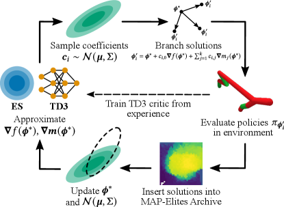
Fig. 1 shows an overview of both algorithms, and Algorithm 1 shows their pseudocode. Since CMA-MEGA (TD3, ES) builds on CMA-MEGA (ES), we include only one algorithm and highlight lines that CMA-MEGA (TD3, ES) additionally executes. The rest of this section reviews the pseudocode in Algorithm 1.

We first set the batch size $\lambda^{\prime}$ for CMA-ES (line 1). While CMA-MEGA (ES) and CMA-MEGA (TD3, ES) both have a total batch size of $\lambda$ solutions on each iteration, one of these solutions is reserved for evaluating ${\bm{\phi}}^{*}$ (line 1). In CMA-MEGA (TD3, ES), an additional solution is reserved for evaluating the greedy actor (line 1). This leaves $\lambda^{\prime}$ solutions remaining for the CMA-ES instance.

Next, we initialize various objects (lines 1-1). CMA-MEGA (TD3, ES) also initializes a replay buffer $\mathcal{B}$ , critic networks $Q_{{\bm{\theta}}_{1}}$ and $Q_{{\bm{\theta}}_{2}}$ , a “greedy” actor $\pi_{{\bm{\phi}}_{q}}$ which is used to train the critics, and target networks $Q_{{\bm{\theta}}^{\prime}_{1}}$ , $Q_{{\bm{\theta}}^{\prime}_{2}}$ , $\pi_{{\bm{\phi}}^{\prime}_{q}}$ (line 1).

In the main loop (line 1), we first evaluate ${\bm{\phi}}^{*}$ (line 1) and insert it into $\mathcal{A}$ (line 1). Then, we estimate the objective and measure gradients of ${\bm{\phi}}^{*}$ with OpenAI-ES (line 1). This estimate computes all objective and measure gradients after evaluating $\lambda_{es}$ solutions (Algorithm 4, Appendix B.2). In CMA-MEGA (TD3, ES), we override the objective gradient estimate with the TD3 estimate (line 1). This estimate samples $n_{pg}$ transitions of experience from $\mathcal{B}$ and computes a gradient ascent step with $Q_{{\bm{\theta}}_{1}}$ (Algorithm 3, Appendix B.2). To make this estimate more accurate, we sample many transitions ( $n_{pg}=65,536$ instead of the default of 100 in TD3 \citepfujimoto2018td3).

Once the gradients are computed, we normalize them to be unit vectors (line 1) and generate $\lambda^{\prime}$ solutions for insertion into $\mathcal{A}$ . Specifically, we sample gradient coefficients ${\bm{c}}$ (line 1), compute perturbation ${\bm{\nabla}}_{i}$ (line 1), and take a gradient step to obtain ${\bm{\phi}}^{\prime}_{i}$ (line 1). Finally, we evaluate ${\bm{\phi}}^{\prime}_{i}$ (line 1) and store the improvement $\Delta_{i}$ (Sec. 3.2.2) from inserting it into $\mathcal{A}$ (line 1).

On line 1, we create an improvement ranking for ${\bm{c}}_{i}$ and ${\bm{\nabla}}_{i}$ based on $\Delta_{i}$ . We update the CMA-ES parameters and ${\bm{\phi}}^{*}$ based on the ranking (lines 1-1). If CMA-ES did not generate any solutions that were inserted into $\mathcal{A}$ , we reset CMA-ES and ${\bm{\phi}}^{*}$ (lines 1-1).

Finally, we update the TD3 instance in CMA-MEGA (TD3, ES). First, identically to PGA-MAP-Elites, we evaluate and insert the greedy actor ${\bm{\phi}}_{q}$ (lines 1-1). Then, we add experience to $\mathcal{B}$ (line 1), including experience from the OpenAI-ES gradient estimate (line 1), and train the critics (line 1). In practice, this training executes in parallel with the rest of the loop to reduce runtime.

4 CMA-MEGA variants $(evaluate,{\bm{\phi}}_{0},N,\lambda,\sigma_{g},\eta,\lambda_{es},\sigma_{e})$ :

Input: Function

evaluate

which executes a policy

{\bm{\phi}}

and outputs objective

f({\bm{\phi}})

and measures

{\bm{m}}({\bm{\phi}})

, initial solution

{\bm{\phi}}_{0}

, desired iterations

N

, batch size

\lambda

, initial CMA-ES step size

\sigma_{g}

, learning rate

\eta

, ES batch size

\lambda_{es}

, ES standard deviation

\sigma_{e}

Result: Generates

N\lambda

solutions, storing elites in an archive

\mathcal{A}

\lambda^{\prime}\leftarrow\lambda-1

\ -\ 1

8 Initialize empty archive

\mathcal{A}

, solution point

{\bm{\phi}}^{*}\leftarrow{\bm{\phi}}_{0}

10 Initialize CMA-ES with population

\lambda^{\prime}

, resulting in

{\bm{\mu}}=\mathbf{0},{\bm{\Sigma}}=\sigma_{g}{\bm{I}}

, and internal CMA-ES parameters

{\bm{p}}

\mathcal{B},Q_{{\bm{\theta}}_{1}},Q_{{\bm{\theta}}_{2}},\pi_{{\bm{\phi}}_{q}},Q_{{\bm{\theta}}^{\prime}_{1}},Q_{{\bm{\theta}}^{\prime}_{2}},\pi_{{\bm{\phi}}^{\prime}_{q}}\leftarrow

Initialize_TD3()

14 for $iter\leftarrow 1..N$ do

f({\bm{\phi}}^{*}),{\bm{m}}({\bm{\phi}}^{*})\leftarrow evaluate({\bm{\phi}}^{*})

16 Update_Archive(

\mathcal{A},{\bm{\phi}}^{*},f({\bm{\phi}}^{*}),{\bm{m}}({\bm{\phi}}^{*})

)

{\bm{\nabla}}f({\bm{\phi}}^{*}),{\bm{\nabla}}{\bm{m}}({\bm{\phi}}^{*})\leftarrow

ES_Gradients(

{\bm{\phi}}^{*},\lambda_{es},\sigma_{e}

)

{\bm{\nabla}}f({\bm{\phi}}^{*})\leftarrow

TD3_Gradient(

{\bm{\phi}}^{*},Q_{{\bm{\theta}}_{1}},\mathcal{B}

)

19 Normalize

{\bm{\nabla}}f({\bm{\phi}}^{*})

and

{\bm{\nabla}}{\bm{m}}({\bm{\phi}}^{*})

to be unit vectors

20 for $i\leftarrow 1..\lambda^{\prime}$ do

{\bm{c}}_{i}\sim\mathcal{N}({\bm{\mu}},{\bm{\Sigma}})

{\bm{\nabla}}_{i}\leftarrow c_{i,0}{\bm{\nabla}}f({\bm{\phi}}^{*})+\sum_{j=1}^{k}c_{i,j}{\bm{\nabla}}m_{j}({\bm{\phi}}^{*})

{\bm{\phi}}^{\prime}_{i}\leftarrow{\bm{\phi}}^{*}+{\bm{\nabla}}_{i}

f({\bm{\phi}}^{\prime}_{i}),{\bm{m}}^{\prime}({\bm{\phi}}^{\prime}_{i})\leftarrow evaluate({\bm{\phi}}^{\prime}_{i})

\Delta_{i}\leftarrow

Update_Archive(

\mathcal{A},{\bm{\phi}}^{\prime}_{i},f({\bm{\phi}}^{\prime}_{i}),{\bm{m}}({\bm{\phi}}^{\prime}_{i})

)

27 end for

29 Rank

{\bm{c}}_{i},{\bm{\nabla}}_{i}

\Delta_{i}

30 Adapt CMA-ES parameters

{\bm{\mu}},{\bm{\Sigma}},{\bm{p}}

based on rankings of

{\bm{c}}_{i}

{\bm{\phi}}^{*}\leftarrow{\bm{\phi}}^{*}+\eta\sum_{i=1}^{\lambda}w_{i}{\bm{\nabla}}_{\text{rank[i]}}

w_{i}

is part of

{\bm{p}}

34 if there is no change in $\mathcal{A}$ then

35 Restart CMA-ES with

{\bm{\mu}}=\mathbf{0},{\bm{\Sigma}}=\sigma_{g}{\bm{I}}

36 Set

{\bm{\phi}}^{*}

to a randomly selected elite from

\mathcal{A}

38 end if

f({\bm{\phi}}_{q}),{\bm{m}}({\bm{\phi}}_{q})\leftarrow evaluate({\bm{\phi}}_{q})

41 Update_Archive(

\mathcal{A},{\bm{\phi}}_{q},f({\bm{\phi}}_{q}),{\bm{m}}({\bm{\phi}}_{q})

)

42 Add experience from all calls to

evaluate

into

\mathcal{B}

43 Train_TD3(

Q_{{\bm{\theta}}_{1}},Q_{{\bm{\theta}}_{2}},\pi_{{\bm{\phi}}_{q}},Q_{{\bm{\theta}}^{\prime}_{1}},Q_{{\bm{\theta}}^{\prime}_{2}},\pi_{{\bm{\phi}}^{\prime}_{q}},\mathcal{B}

)

45 end for

Algorithm 1 CMA-MEGA (ES) and CMA-MEGA (TD3, ES). Highlighted portions are only executed in CMA-MEGA (TD3, ES). Adapted from CMA-MEGA \citepfontaine2021dqd. Refer to Appendix B.2 for functions whose names are in Small_Caps.

B.2 Helper Methods for CMA-MEGA Variants

1 Update_Archive $(\mathcal{A},{\bm{\phi}},f({\bm{\phi}}),{\bm{m}}({\bm{\phi}}))$ :

2 //

\mathcal{E}

contains

{\bm{\phi}}_{\mathcal{E}},f({\bm{\phi}}_{\mathcal{E}}),{\bm{m}}({\bm{\phi}}_{\mathcal{E}})

\mathcal{E}\leftarrow

cell in

\mathcal{A}

corresponding to

{\bm{m}}

4 if $\mathcal{E}$ is empty then

{\bm{\phi}}_{\mathcal{E}},f({\bm{\phi}}_{\mathcal{E}}),{\bm{m}}({\bm{\phi}}_{\mathcal{E}})\leftarrow{\bm{\phi}},f({\bm{\phi}}),{\bm{m}}({\bm{\phi}})

6 return (new_cell,

f({\bm{\phi}})

)

8 else if $f({\bm{\phi}})>f({\bm{\phi}}_{\mathcal{E}})$ then

{\bm{\phi}}_{\mathcal{E}},f({\bm{\phi}}_{\mathcal{E}}),{\bm{m}}({\bm{\phi}}_{\mathcal{E}})\leftarrow{\bm{\phi}},f({\bm{\phi}}),{\bm{m}}({\bm{\phi}})

10 return (improve_existing_cell,

f({\bm{\phi}})-f({\bm{\phi}}_{\mathcal{E}})

)

11 else

12 return (not_added,

f({\bm{\phi}})-f({\bm{\phi}}_{\mathcal{E}})

)

13 end if

Algorithm 2 Helper function for updating the archive.

2 Initialize_TD3 :

\mathcal{B}\leftarrow

initialize_replay_buffer()

4 // As done in the TD3 author implementation \citepfujimoto2018td3, we initialize these networks with the default PyTorch weights.

Q_{{\bm{\theta}}_{1}},Q_{{\bm{\theta}}_{2}},\pi_{{\bm{\phi}}_{q}}\leftarrow

initialize_networks()

Q_{{\bm{\theta}}^{\prime}_{1}},Q_{{\bm{\theta}}^{\prime}_{2}},\pi_{{\bm{\phi}}^{\prime}_{q}}\leftarrow Q_{{\bm{\theta}}_{1}},Q_{{\bm{\theta}}_{2}},\pi_{{\bm{\phi}}_{q}}

7 return $\mathcal{B},Q_{{\bm{\theta}}_{1}},Q_{{\bm{\theta}}_{2}},\pi_{{\bm{\phi}}_{q}},Q_{{\bm{\theta}}^{\prime}_{1}},Q_{{\bm{\theta}}^{\prime}_{2}},\pi_{{\bm{\phi}}^{\prime}_{q}}$

11 TD3_Gradient ( ${\bm{\phi}},Q_{{\bm{\theta}}_{1}},\mathcal{B}$ ):

12 Sample

n_{pg}

transitions

(s_{t},a_{t},r(s_{t},a_{t}),s_{t+1})

from

\mathcal{B}

\nabla_{\bm{\phi}}J({\bm{\phi}})=\frac{1}{n_{pg}}\sum\nabla_{\bm{\phi}}\pi_{\bm{\phi}}(s_{t})\nabla_{a}Q_{{\bm{\theta}}_{1}}(s_{t},a)|_{a=\pi_{\bm{\phi}}(s_{t})}

14 return $\nabla_{\bm{\phi}}J({\bm{\phi}})$

18 Train_TD3 $(Q_{{\bm{\theta}}_{1}},Q_{{\bm{\theta}}_{2}},\pi_{{\bm{\phi}}_{q}}Q_{{\bm{\theta}}^{\prime}_{1}},Q_{{\bm{\theta}}^{\prime}_{2}},\pi_{{\bm{\phi}}^{\prime}_{q}},\mathcal{B})$ :

19 // Trains the critic and the greedy actor.

20 for $i\leftarrow 1..n_{crit}$ do

21 Sample

n_{q}

transitions

(s_{t},a_{t},r(s_{t},a_{t}),s_{t+1})

from

\mathcal{B}

22 // Sample smoothing noise.

\epsilon\sim

clip

(\mathcal{N}(0,\sigma_{p}),-c_{clip},c_{clip})

y=r(s_{t},a_{t})+\gamma\min_{i=1,2}Q_{{\bm{\theta}}^{\prime}_{i}}(s_{t+1},\pi_{{\bm{\phi}}^{\prime}_{q}}(s_{t+1})+\epsilon)

25 // Update critics.

{\bm{\theta}}_{i}\leftarrow\operatorname*{arg\,min}_{{\bm{\theta}}_{i}}\frac{1}{n_{q}}\sum(y-Q_{{\bm{\theta}}_{i}}(s_{t},a_{t}))^{2}

27 if $t\mod d=0$ then

28 // Update greedy actor.

\nabla_{{\bm{\phi}}_{q}}J({\bm{\phi}}_{q})=\frac{1}{n_{q}}\sum\nabla_{{\bm{\phi}}_{q}}\pi_{{\bm{\phi}}_{q}}(s_{t})\nabla_{a}Q_{{\bm{\theta}}_{1}}(s_{t},a)|_{a=\pi_{{\bm{\phi}}_{q}}(s_{t})}

30 // Update targets.

{\bm{\theta}}^{\prime}_{i}\leftarrow\tau{\bm{\theta}}_{i}+(1-\tau){\bm{\theta}}^{\prime}_{i}

{\bm{\phi}}^{\prime}_{q}\leftarrow\tau{\bm{\phi}}_{q}+(1-\tau){\bm{\phi}}^{\prime}_{q}

34 end if

36 end for

Algorithm 3 TD3 helper functions. Adapted from PGA-MAP-Elites \citepnilsson2021pga and TD3 \citepfujimoto2018td3.

1 ES_Gradients $({\bm{\phi}},\lambda_{es},\sigma_{e})$ :

2 // Mirror sampling - divide

\lambda_{es}

by 2.

3 for $i\leftarrow 1..\frac{\lambda_{es}}{2}$ do

{\bm{\epsilon}}_{i}\sim{\mathcal{N}}(\mathbf{0},{\bm{I}})

{\bm{x}}_{i}\leftarrow{\bm{\phi}}+\sigma_{e}{\bm{\epsilon}}_{i}

f({\bm{x}}_{i}),{\bm{m}}({\bm{x}}_{i})\leftarrow evaluate({\bm{x}}_{i})

{\bm{x}}^{\prime}_{i}\leftarrow{\bm{\phi}}-\sigma_{e}{\bm{\epsilon}}_{i}

8 //

{\bm{x}}^{\prime}_{i}

reflects

{\bm{x}}_{i}

f({\bm{x}}^{\prime}_{i}),{\bm{m}}({\bm{x}}^{\prime}_{i})\leftarrow evaluate({\bm{x}}_{i})

11 end for

13 for $j\leftarrow 0..k$ do

14 if $j=0$ then

L\leftarrow

all

{\bm{x}}_{i}

and

{\bm{x}}^{\prime}_{i}

, sorted by

f

16 else

L\leftarrow

all

{\bm{x}}_{i}

and

{\bm{x}}^{\prime}_{i}

, sorted by

m_{j}

18 end if

19 // Rank normalization.

R\leftarrow

rank (index) of every

{\bm{x}}_{i}

L

R^{\prime}\leftarrow

rank (index) of every

{\bm{x}}^{\prime}_{i}

L

22 // Ranks should be normalized over both lists combined (

R\|R^{\prime}

) rather than in each list separately.

23 Normalize ranks in

R\|R^{\prime}

[-0.5,0.5]

25 // Estimate gradient.

{\bm{\nabla}}\leftarrow\frac{1}{\frac{\lambda_{es}}{2}\sigma_{e}}\sum_{i=1}^{\frac{\lambda_{es}}{2}}{\bm{\epsilon}}_{i}(R_{i}-R^{\prime}_{i})

27 if $j=0$ then

{\bm{\nabla}}f({\bm{\phi}})\leftarrow{\bm{\nabla}}

29 else

{\bm{\nabla}}{m_{j}}({\bm{\phi}})\leftarrow{\bm{\nabla}}

31 end if

33 end for

35 return ${\bm{\nabla}}f({\bm{\phi}}),{\bm{\nabla}}{\bm{m}}({\bm{\phi}})$

Algorithm 4 Helper function for estimating objective and measure gradients with the gradient estimate from OpenAI-ES. This implementation differs from Eq. 3 since it includes mirror sampling and rank normalization.

Appendix C Algorithm Hyperparameters

Here we list parameters for each algorithm in our experiments. Refer to Sec. 5.1.2 for parameters of the neural network policy and the archive. All algorithms are allocated 1,000,000 evaluations total.

Table 1: CMA-MEGA (ES) and CMA-MEGA (TD3, ES) hyperparameters.

n_{pg}

and

n_{crit}

are only applicable in CMA-MEGA (TD3, ES).

n_{pg}

here is analogous to

n_{pg}

in PGA-MAP-Elites, but it is much larger here since we only compute one gradient per iteration instead of taking gradient steps on multiple solutions.

Parameter	Description	Value
$N$	Iterations = 1,000,000 / ( $\lambda+\lambda_{es}$ )	5,000
$\lambda$	Batch size	100
$\sigma_{g}$	Initial CMA-ES step size	1.0
$\eta$	Gradient ascent learning rate	1.0
$\lambda_{es}$	ES batch size	100
$\sigma_{e}$	ES noise standard deviation	0.02
$n_{pg}$	TD3 gradient estimate batch size	65,536
$n_{crit}$	TD3 critic training steps	600

Table 2: PGA-MAP-Elites hyperparameters.

Parameter	Description	Value
$N$	Iterations = 1,000,000 / $\lambda$	10,000
$\lambda$	Batch size	100
$n_{evo}$	Variation operators split	$0.5\lambda=50$
$n_{grad}$	PG variation steps	10
$\alpha_{grad}$	PG variation learning rate (for Adam)	0.001
$n_{pg}$	PG variation batch size	256
$n_{crit}$	TD3 critic training steps	300
$\sigma_{1}$	GA variation 1	0.005
$\sigma_{2}$	GA variation 2	0.05
$G$	Random initial solutions	100

Table 3: ME-ES hyperparameters. We adopt the explore-exploit variant.

Parameter	Description	Value
$N$	Iterations = 1,000,000 / $\lambda$	5,000
$\lambda$	Batch size	200
$\sigma$	ES noise standard deviation	0.02
$n_{optim\_gens}$	Consecutive generations to optimize a solution	10
$\alpha$	Learning rate for Adam	0.01
$\alpha_{2}$	L2 coefficient for Adam	0.005
$k$	Nearest neighbors for novelty calculation	10

Table 4: MAP-Elites hyperparameters. We describe MAP-Elites in Sec. 3.2.1.

Parameter	Description	Value
$N$	Iterations = 1,000,000 / $\lambda$	10,000
$\lambda$	Batch size	100
$\sigma$	Gaussian noise standard deviation	0.02

Table 5: TD3 hyperparameters common to CMA-MEGA (TD3, ES) and PGA-MAP-Elites, which both train a TD3 instance. Furthermore, though we record the objective with

\gamma=1

(Sec. 5.1.3), TD3 still executes with

\gamma<1

Parameter	Description	Value
—	Critic layer sizes	$[256,256,1]$
$\alpha_{crit}$	Critic learning rate (for Adam)	3e-4
$n_{q}$	Critic training batch size	256
$\|\mathcal{B}\|$	Max replay buffer size	1,000,000
$\gamma$	Discount factor	0.99
$\tau$	Target network update rate	0.005
$d$	Target network update frequency	2
$\sigma_{p}$	Smoothing noise standard deviation	0.2
$c_{clip}$	Smoothing noise clip	0.5

Appendix D Environment Details

D.1 Measures

The measures in QDGym are the proportions of time that each foot contacts the ground. In each environment, the feet are ordered as follows:

•

QD Ant: front left foot, front right foot, back left foot, back right foot
•

QD Half-Cheetah: front foot, back foot
•

QD Hopper: single foot
•

QD Walker: right foot, left foot

Appendix E Final Metrics

Tables 6-11 show the QD score (Sec. 5.1.3), QD score AUC (Sec. G.1.1), archive coverage (Sec. 5.1.3), best performance (Sec. 5.1.3), mean elite robustness (Sec. G.3), and runtime in hours (Sec. G.5) for all algorithms in all environments. The tables show the value of each metric after 1 million evaluations, averaged over 5 trials. Due to its magnitude, QD score AUC is expressed as a multiple of $10^{12}$ .

Table 6: QD Score

	QD Ant	QD Half-Cheetah	QD Hopper	QD Walker
CMA-MEGA (ES)	1,649,846.69	4,489,327.04	1,016,897.48	371,804.19
CMA-MEGA (TD3, ES)	1,479,725.62	4,612,926.99	1,857,671.12	1,437,319.62
PGA-MAP-Elites	1,674,374.81	4,758,921.89	2,068,953.54	1,480,443.84
ME-ES	539,742.08	2,296,974.58	791,954.55	105,320.97
MAP-Elites	1,418,306.56	4,175,704.19	1,835,703.73	447,737.90

Table 7: QD Score AUC (multiple of

10^{12}

)

	QD Ant	QD Half-Cheetah	QD Hopper	QD Walker
CMA-MEGA (ES)	1.31	3.96	0.74	0.28
CMA-MEGA (TD3, ES)	1.14	3.97	1.39	1.01
PGA-MAP-Elites	1.39	4.39	1.81	1.04
ME-ES	0.35	1.57	0.49	0.07
MAP-Elites	1.18	3.78	1.34	0.35

Table 8: Archive Coverage

	QD Ant	QD Half-Cheetah	QD Hopper	QD Walker
CMA-MEGA (ES)	0.96	1.00	0.97	1.00
CMA-MEGA (TD3, ES)	0.97	1.00	0.98	1.00
PGA-MAP-Elites	0.96	1.00	0.97	0.99
ME-ES	0.63	0.95	0.74	0.86
MAP-Elites	0.98	1.00	0.98	1.00

Table 9: Best Performance

	QD Ant	QD Half-Cheetah	QD Hopper	QD Walker
CMA-MEGA (ES)	2,213.06	2,265.73	1,441.00	940.50
CMA-MEGA (TD3, ES)	2,482.83	2,486.10	2,597.87	2,302.31
PGA-MAP-Elites	2,843.86	2,746.98	2,884.08	2,619.17
ME-ES	2,515.20	1,911.33	2,642.30	1,025.74
MAP-Elites	1,506.97	1,822.88	2,602.94	989.31

Table 10: Mean Elite Robustness

	QD Ant	QD Half-Cheetah	QD Hopper	QD Walker
CMA-MEGA (ES)	-51.62	-105.81	-187.44	-86.45
CMA-MEGA (TD3, ES)	-48.91	-80.78	-273.68	-97.40
PGA-MAP-Elites	-4.16	-92.38	-435.45	-74.26
ME-ES	77.76	-645.40	-631.32	2.05
MAP-Elites	-109.42	-338.78	-509.21	-186.14

Table 11: Runtime (Hours)

	QD Ant	QD Half-Cheetah	QD Hopper	QD Walker
CMA-MEGA (ES)	7.40	7.24	3.84	3.52
CMA-MEGA (TD3, ES)	16.26	22.79	13.43	13.01
PGA-MAP-Elites	19.99	19.75	12.65	12.86
ME-ES	8.92	10.25	4.04	4.12
MAP-Elites	7.43	7.37	4.59	5.72

Appendix F Full Statistical Analysis

To compare a metric such as QD score between two or more algorithms across all four QDGym environments, we performed a two-way ANOVA where environment and algorithm were the independent variables and the metric was the dependent variable. When there was a significant interaction effect (note that all of our analyses found significant interaction effects), we followed up this ANOVA with a simple main effects analysis in each environment. Finally, we ran pairwise comparisons (two-sided t-tests) to determine which algorithms had a significant difference on the metric. We applied Bonferroni corrections within each environment / simple main effect. For example, in Table 12 we compared CMA-MEGA (ES) with three algorithms in each environment, so we applied a Bonferroni correction with $n=3$ .

This section lists the ANOVA and pairwise comparison results for each of our analyses. We have bolded all significant $p$ -values, where significance is determined at the $\alpha=0.05$ threshold. For pairwise comparisons, some $p$ -values are marked as “1” because the Bonferroni correction caused the $p$ -value to exceed 1. $p$ -values less than 0.001 have been marked as “< 0.001”.

F.1 QD Score Analysis (Sec. G.1)

To test the hypotheses we defined in Sec. 5.2, we performed a two-way ANOVA for QD scores. Since the ANOVA requires scores in all environments to have the same scale, we normalized the QD score in all environments by dividing by the maximum QD score, defined in Sec. G.1 as grid cells * (max objective - min objective). The results of the ANOVA were as follows:

•

Interaction effect: $F(12,80)=16.82,\mathbf{p<0.001}$
•
Simple main effects:
- –
  
  QD Ant: $F(4,80)=23.87,\mathbf{p<0.001}$
- –
  
  QD Half-Cheetah: $F(4,80)=44.15,\mathbf{p<0.001}$
- –
  
  QD Hopper: $F(4,80)=57.35,\mathbf{p<0.001}$
- –
  
  QD Walker: $F(4,80)=90.84,\mathbf{p<0.001}$

Since the ANOVA showed a significant interaction effect and significant simple main effects, we performed pairwise comparisons for each hypothesis (Tables 12-14).

F.2 QD Score AUC Analysis (Sec. G.1.1)

In this followup analysis, we hypothesized that PGA-MAP-Elites would have greater QD score AUC than CMA-MEGA (ES) and CMA-MEGA (TD3, ES). Thus, we performed a two-way ANOVA which compared QD score AUC for PGA-MAP-Elites, CMA-MEGA (ES), and CMA-MEGA (TD3, ES). As we did for QD score, we normalized QD score AUC by the maximum QD score. The ANOVA results were as follows:

•

Interaction effect: $F(12,80)=17.55,\mathbf{p<0.001}$
•
Simple main effects:
- –
  
  QD Ant: $F(4,80)=31.77,\mathbf{p<0.001}$
- –
  
  QD Half-Cheetah: $F(4,80)=89.38,\mathbf{p<0.001}$
- –
  
  QD Hopper: $F(4,80)=82.34,\mathbf{p<0.001}$
- –
  
  QD Walker: $F(4,80)=71.64,\mathbf{p<0.001}$

As the interaction and simple main effects were significant, we performed pairwise comparisons (Table 15).

F.3 Mean Elite Robustness Analysis (Sec. G.3)

In this followup analysis, we hypothesized that MAP-Elites would have lower mean elite robustness than CMA-MEGA (ES) and CMA-MEGA (TD3, ES). Thus, we performed a two-way ANOVA which compared mean elite robustness for MAP-Elites, CMA-MEGA (ES), and CMA-MEGA (TD3, ES). We normalized by the score range, i.e. max objective - min objective. The ANOVA results were as follows:

•

Interaction effect: $F(12,80)=8.75,\mathbf{p<0.001}$
•
Simple main effects:
- –
  
  QD Ant: $F(4,80)=3.17,\mathbf{p=0.018}$
- –
  
  QD Half-Cheetah: $F(4,80)=9.60,\mathbf{p<0.001}$
- –
  
  QD Hopper: $F(4,80)=21.07,\mathbf{p<0.001}$
- –
  
  QD Walker: $F(4,80)=3.70,\mathbf{p=0.008}$

As the interaction and simple main effects were significant, we performed pairwise comparisons (Table 16).

Table 12: H1 - Comparing QD score between CMA-MEGA (ES) and baselines

		QD Ant	QD Half-Cheetah	QD Hopper	QD Walker
Algorithm 1	Algorithm 2
CMA-MEGA (ES)	PGA-MAP-Elites	1	0.733	0.003	< 0.001
	ME-ES	< 0.001	< 0.001	0.841	< 0.001
	MAP-Elites	0.254	0.215	0.007	0.108

Table 13: H2 - Comparing QD score between CMA-MEGA (TD3, ES) and baselines

		QD Ant	QD Half-Cheetah	QD Hopper	QD Walker
Algorithm 1	Algorithm 2
CMA-MEGA (TD3, ES)	PGA-MAP-Elites	0.093	1	0.726	1
	ME-ES	< 0.001	< 0.001	< 0.001	< 0.001
	MAP-Elites	1	0.010	1	< 0.001

Table 14: H3 - Comparing QD score between CMA-MEGA (ES) and CMA-MEGA (TD3, ES)

		QD Ant	QD Half-Cheetah	QD Hopper	QD Walker
Algorithm 1	Algorithm 2
CMA-MEGA (ES)	CMA-MEGA (TD3, ES)	0.250	0.511	0.006	< 0.001

Table 15: Comparing QD score AUC between PGA-ME and CMA-MEGA variants

		QD Ant	QD Half-Cheetah	QD Hopper	QD Walker
Algorithm 1	Algorithm 2
PGA-MAP-Elites	CMA-MEGA (ES)	0.734	0.255	< 0.001	< 0.001
	CMA-MEGA (TD3, ES)	0.020	0.111	0.003	1

Table 16: Comparing mean elite robustness between MAP-Elites and CMA-MEGA variants

		QD Ant	QD Half-Cheetah	QD Hopper	QD Walker
Algorithm 1	Algorithm 2
MAP-Elites	CMA-MEGA (ES)	< 0.001	< 0.001	0.030	0.003
	CMA-MEGA (TD3, ES)	< 0.001	< 0.001	0.013	< 0.001

Appendix G Discussion

G.1 Analysis

To test our hypotheses, we conducted a two-way ANOVA which examined the effect of algorithm and environment on the QD score. We note that the ANOVA requires QD scores to have the same scale, but each environment’s QD score has a different scale by default. Thus, for this analysis, we normalized QD scores by dividing by each environment’s maximum QD score, defined as grid cells * (max objective - min objective) (see Table LABEL:table:envs for these quantities).

We found a statistically significant interaction between algorithm and environment on QD score, $F(12,80)=16.82,p<0.001$ . Simple main effects analysis indicated that the algorithm had a significant effect on QD score in each environment, so we ran pairwise comparisons (two-sided t-tests) with Bonferroni corrections (Appendix F). Our results are as follows:

•

H1: There is no significant difference in QD score between CMA-MEGA (ES) and PGA-MAP-Elites in QD Ant and QD Half-Cheetah, but in QD Hopper and QD Walker, CMA-MEGA (ES) attains significantly lower QD score than PGA-MAP-Elites. CMA-MEGA (ES) achieves significantly higher QD score than ME-ES in all environments except QD Hopper, where there is no significant difference. There is no significant difference between CMA-MEGA (ES) and MAP-Elites in all domains except QD Hopper, where CMA-MEGA (ES) attains significantly lower QD score.
•

H2: In all environments, there is no significant difference in QD score between CMA-MEGA (TD3, ES) and PGA-MAP-Elites. CMA-MEGA (TD3, ES) achieves significantly higher QD score than ME-ES in all environments. CMA-MEGA (TD3, ES) achieves significantly higher QD score than MAP-Elites in QD Half-Cheetah and QD Walker, but there is no significant difference in QD Ant and QD Hopper.
•

H3: CMA-MEGA (TD3, ES) achieves significantly higher QD score than CMA-MEGA (ES) in QD Hopper and QD Walker, but there is no significant difference in QD Ant and QD Half-Cheetah.

G.1.1 PGA-MAP-Elites and objective-measure space exploration

Of the CMA-MEGA variants, CMA-MEGA (TD3, ES) performed the closest to PGA-MAP-Elites, with no significant QD score difference in any environment. This result differs from prior work \citepfontaine2021dqd in QD benchmark domains, where CMA-MEGA outperformed OG-MAP-Elites, a baseline DQD algorithm inspired by PGA-MAP-Elites.

We attribute this difference to the difficulty of exploring objective-measure space in the benchmark domains. For example, the linear projection benchmark domain is designed to be “distorted” \citepfontaine2020covariance. Values in the center of its measure space are easy to obtain with random sampling, while values at the edges are unlikely to be sampled. Hence, high QD score arises from traversing measure space and filling the archive. In contrast, as discussed in Sec. 5.1.1, it is relatively easy to fill the archive in QDGym. We see this empirically — in all environments, all algorithms achieve nearly 100% archive coverage. This may even happen within the first 100k evaluations, as in QD Half-Cheetah (Fig. 3). Hence, high QD score in QDGym comes from optimizing solutions after filling the archive.

Since CMA-MEGA adapts its sampling distribution, it performs the exploration necessary to succeed in the linear projection domain, while OG-MAP-Elites remains “stuck” in the center of the measure space. However, this exploration capability does not increase QD score in QDGym. Instead, QDGym is more appropriate for an algorithm which rigorously optimizes the objective. PGA-MAP-Elites does exactly this: every iteration, it increases the objective value of half of its generated solutions by optimizing them with respect to a TD3 critic. Though CMA-MEGA (TD3, ES) also trains a TD3 critic, it does not perform this additional optimization. Naturally, this leads to a possible extension in which solutions sampled by CMA-MEGA (TD3, ES) are optimized with respect to its TD3 critic before being evaluated in the environment.

G.1.2 PGA-MAP-Elites and optimization efficiency

While there was no significant difference in the final QD scores of CMA-MEGA (TD3, ES) and PGA-MAP-Elites, CMA-MEGA (TD3, ES) was less efficient than PGA-MAP-Elites in some environments. For instance, in QD Hopper, PGA-MAP-Elites reached 1.5M QD score after 100k evaluations, but CMA-MEGA (TD3, ES) required 400k evaluations.

We can quantify optimization efficiency with QD score AUC, the area under the curve (AUC) of the QD score plot. For a QD algorithm which executes $N$ iterations and evaluates $\lambda$ solutions per iteration, we define QD score AUC as a Riemann sum:

\displaystyle\text{QD score AUC}=\sum_{i=1}^{N}(\lambda*\text{QD score at iteration $i$})

(4)

After computing QD score AUC, we ran statistical analysis similar to Sec. G.1 and found CMA-MEGA (TD3, ES) had significantly lower QD score AUC than PGA-MAP-Elites in QD Ant and QD Hopper. There was no significant difference in QD Half-Cheetah and QD Walker. As such, while CMA-MEGA (TD3, ES) obtained comparable final QD scores to PGA-MAP-Elites in all tasks, it was less efficient at achieving those scores in QD Ant and QD Hopper.

G.2 ME-ES and archive insertions

With one exception (CMA-MEGA (ES) in QD Hopper), both CMA-MEGA variants achieved significantly higher QD score than ME-ES in all environments. We attribute this result to the number of solutions each algorithm inserts into the archive. Each iteration, ME-ES evaluates 200 solutions (Appendix C) but only inserts one into the archive, for a total of 5000 solutions inserted during each run. Given that each archive has at least 1000 cells, ME-ES has, on average, 5 opportunities to insert a solution that improves each cell. In contrast, the CMA-MEGA variants have 100 times more insertions. Though the variants also evaluate 200 solutions per iteration, they insert 100 of these into the archive. This totals to 500k insertions per run, allowing the variants to gradually improve archive cells.

G.3 MAP-Elites and robustness

In most cases, both CMA-MEGA variants had significantly higher QD score than MAP-Elites or no significant difference, but in QD Hopper, MAP-Elites achieved significantly higher QD score than CMA-MEGA (ES). However, when we visualized solutions found by MAP-Elites, their performance was lower than the performance recorded in the archive. The best MAP-Elites solution in QD Hopper hopped forward a few steps and fell down, despite recording an excellent performance of 2,648.31 (see supplemental videos).

One explanation for this behavior is that since we only evaluate solutions for one episode before inserting into the archive, a solution with noisy performance may be inserted because of a single high-performing episode, even if it performs poorly on average. Prior work \citepnilsson2021pga has also encountered this issue when running MAP-Elites with a directional variation operator \citepvassiliades2018line in QDGym, and has suggested measuring robustness as a proxy for how much noise is present in an archive’s solutions. Robustness is defined as the difference between the mean performance of the solution over $n$ episodes (we use $n=10$ ) and the performance recorded in the archive. The larger (more negative) this difference, the more noisy and less robust the solution.

To compare the robustness of the solutions output by the CMA-MEGA variants and MAP-Elites, we computed mean elite robustness, the average robustness of all elites in each experiment’s final archive. We then ran statistical analysis similar to Sec. G.1. In all environments, both CMA-MEGA (ES) and CMA-MEGA (TD3, ES) had significantly higher mean elite robustness than MAP-Elites (Appendix E & F). Overall, though MAP-Elites achieves high QD score, its solutions are less robust.

G.4 CMA-MEGA variants and gradient estimates

In QD Hopper and QD Walker, CMA-MEGA (TD3, ES) had significantly higher QD score than CMA-MEGA (ES). One potential explanation is that PyBullet Gym (and hence QDGym) augments rewards with reward shaping signals intended to promote optimal solutions for deep RL algorithms. In prior work \citeppagliuca2020, these signals led PPO \citepschulman2017ppo to train successful walking agents, while they led OpenAI-ES into local optima. For instance, OpenAI-ES trained agents which stood still so as to maximize only the reward signal for staying upright.

Due to these signals, TD3’s objective gradient seems more useful than that of OpenAI-ES in QD Hopper and QD Walker. In fact, the algorithms which performed best in QD Hopper and QD Walker were ones that calculated objective gradients with TD3, i.e. PGA-MAP-Elites and CMA-MEGA (TD3, ES).

Prior work \citeppagliuca2020 found that rewards could be tailored for ES, such that OpenAI-ES outperformed PPO. Extensions of our work could investigate whether there is a similar effect for QD algorithms, where tailoring the reward leads CMA-MEGA (ES) to outperform PGA-MAP-Elites and CMA-MEGA (TD3, ES).

G.5 Computational effort

Though CMA-MEGA (TD3, ES) and PGA-MAP-Elites perform best overall, they rely on specialized hardware (a GPU) and require the most computation. As shown in Table 11, Appendix E, the TD3 training in these algorithms leads to long runtimes. When runtime is dominated by the algorithm itself (as opposed to solution evaluations), CMA-MEGA (ES) offers a viable alternative that may achieve reasonable performance.

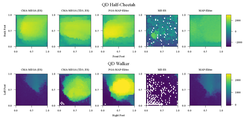
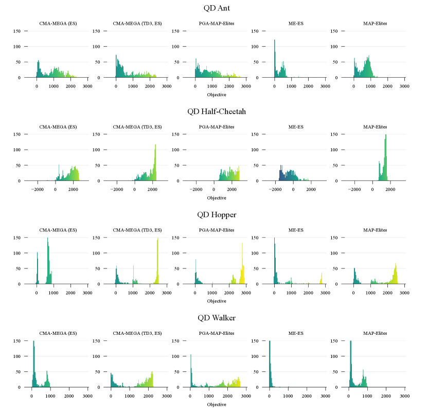
Appendix H Archive Visualizations

We visualize “median” archives in Fig. 5 and Fig. 6. To determine these median archives, we selected the trial which achieved the median QD score out of the 5 trials of each algorithm in each environment. Fig. 5 visualizes heatmaps of median archives in QD Half-Cheetah and QD Walker, while Fig. 6 shows the distribution (histogram) of objective values for median archives in all environments. Refer to the supplemental material for videos of how these figures develop across iterations.

Differentiable Quality Diversity for Reinforcement Learning by Approximating Gradients