Differentiable Top- Classification Learning
Abstract
The top- classification accuracy is one of the core metrics in machine learning. Here, is conventionally a positive integer, such as or , leading to top- or top- training objectives. In this work, we relax this assumption and optimize the model for multiple simultaneously instead of using a single . Leveraging recent advances in differentiable sorting and ranking, we propose a differentiable top- cross-entropy classification loss. This allows training the network while not only considering the top- prediction, but also, e.g., the top- and top- predictions. We evaluate the proposed loss function for fine-tuning on state-of-the-art architectures, as well as for training from scratch. We find that relaxing does not only produce better top- accuracies, but also leads to top- accuracy improvements. When fine-tuning publicly available ImageNet models, we achieve a new state-of-the-art for these models.
1 Introduction
Classification is one of the core disciplines in machine learning and computer vision. The advent of classification problems with hundreds or even thousands of classes let the top- classification accuracy establish as an important metric, i.e., one of the top- classes has to be the correct class. Usually, models are trained to optimize the top- accuracy; and top- etc. are used for evaluation only. Some works (Lapin et al., 2016; Berrada et al., 2018) have challenged this idea and proposed top- losses, such as a smooth top- margin loss. These methods have demonstrated superior robustness over the established top- softmax cross-entropy in the presence of additional label noise (Berrada et al., 2018). In standard classification settings, however, these methods have so far not shown improvements over the established top- softmax cross-entropy.
In this work, instead of selecting a single top- metric such as top- or top- for defining the loss, we propose to specify to be drawn from a distribution , which may or may not depend on the confidence of specific data points or on the class label. Examples for distributions are ( top- and top-), ( top- and top-), and ( top- for each from to ). Note that, when is drawn from a distribution, this is done sampling-free as we can compute the expectation value in closed form.
Conventionally, given scores returned by a neural network, softmax produces a probability distribution over the top- rank. Recent advances in differentiable sorting and ranking (Grover et al., 2019; Prillo & Eisenschlos, 2020; Cuturi et al., 2019; Petersen et al., 2021a) provide methods for generalizing this to probability distributions over all ranks represented by a matrix . Based on differentiable ranking, multiple differentiable top- operators have recently been proposed. They found applications in differentiable -nearest neighbor algorithms, differentiable beam search, attention mechanisms, and differentiable image patch selection (Cordonnier et al., 2021). In these areas, integrating differentiable top- improved results considerably by creating a more natural end-to-end learning setting. However, to date, none of the differentiable top- operators have been employed as neural network losses for top- classification learning with .
Building on differentiable sorting and ranking methods, we propose a new family of differentiable top- classification losses where is drawn from a probability distribution. We find that our top- losses improve not only top- accuracies, but also top- accuracy on multiple learning tasks.
We empirically evaluate our method using four differentiable sorting and ranking methods on the CIFAR-100 (Krizhevsky et al., 2009), the ImageNet-1K (Deng et al., 2009), and the ImageNet-21K-P (Ridnik et al., 2021) data sets. Using CIFAR-100, we demonstrate the capabilities of our losses to train models from scratch. On ImageNet-1K, we demonstrate that our losses are capable of fine-tuning existing models and achieve a new state-of-the-art for publicly available models on both top- and top- accuracy. We benchmark our method on multiple recent models and demonstrate that our proposed method consistently outperforms the baselines for the best two differentiable sorting and ranking methods. With ImageNet-21K-P, where many classes overlap (but only one is the ground truth), we demonstrate that our losses are scalable to more than classes and achieve improvements of over with only last layer fine-tuning.
Overall, while the performance improvements on fine-tuning are rather limited (because we retrain only the classification head), they are consistent and can be achieved without the large costs of training from scratch. The absolute improvement that we achieve on the ResNeXt-101 32x48d WSL top- accuracy corresponds to an error reduction by approximately , and can be achieved at much less than the computational cost of (re-)training the full model in the first place.
We summarize our contributions as follows:
-
•
We derive a novel family of top- cross-entropy losses and relax the assumption of a fixed .
-
•
We find that they improve both top- and top- accuracy.
-
•
We demonstrate that our losses are scalable to more than classes.
-
•
We propose splitter selection nets, which require fewer layers than existing selection nets.
-
•
We achieve new state-of-the-art results (for publicly available models) on ImageNet1K.
2 Background: Differentiable Sorting and Ranking
We briefly review NeuralSort, SoftSort, Optimal Transport Sort, and Differentiable Sorting Networks. We omit the fast differentiable sorting and ranking method (Blondel et al., 2020) and the relaxed Bubble sort algorithm (Petersen et al., 2021b) as they do not provide relaxed permutation matrices / probability scores, but rather only sorted / ranked vectors.
2.1 NeuralSort & SoftSort
To make the sorting operation differentiable, Grover et al. (2019) proposed relaxing permutation matrices to unimodal row-stochastic matrices. For this, they use the softmax of pairwise differences of (cumulative) sums of the top elements. They prove that this, for the temperature parameter approaching , is the correct permutation matrix, and propose a variety of deep learning differentiable sorting benchmark tasks. They propose a deterministic softmax-based variant, as well as a Gumbel-Softmax variant of their algorithm. Note that NeuralSort is not based on sorting networks.
Prillo & Eisenschlos (2020) build on this idea but simplify the formulation and provide SoftSort, a faster alternative to NeuralSort. They show that it is sufficient to build on pairwise differences of elements of the vectors to be sorted instead of the cumulative sums. They find that SoftSort performs approximately equivalent in their experiments to NeuralSort.
2.2 Optimal Transport / Sinkhorn Sort
Cuturi et al. (2019) propose an entropy regularized optimal transport formulation of the sorting operation. They solve this by applying the Sinkhorn algorithm (Cuturi, 2013) and produce gradients via automatic differentiation rather than the implicit function theorem, which resolves the need of solving a linear equation system. As the Sinkhorn algorithm produces a relaxed permutation matrix, we can also apply Sinkhorn sort to top- classification learning.
2.3 Differentiable Sorting Networks
Petersen et al. (2021a) propose differentiable sorting networks, a continuous relaxation of sorting networks. Sorting networks are a kind of sorting algorithm that consist of wires carrying the values and comparators, which swap the values on two wires if they are not in the desired order. Sorting networks can be made differentiable by perturbing the values on the wires in each layer of the sorting network by a logistic distribution, i.e., instead of and they use and . Similar to the methods above, this method produces a relaxed permutation matrix, which allows us to apply it to top- classification learning. The method has also been improved by enforcing monotonicity and bounding the approximation error (Petersen et al., 2022). Note that sorting networks are a classic algorithmic concept (Knuth, 1998), are not neural networks nor refer to differentiable sorting. Differentiable sorting networks are one of multiple differentiable sorting and ranking methods.
3 Top- Learning
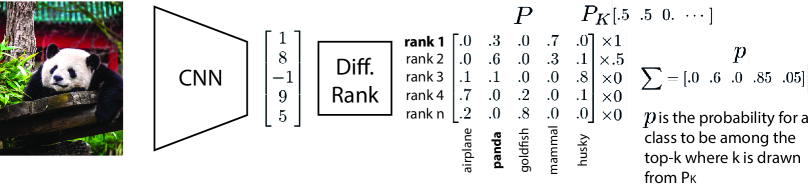
In this section, we start by introducing our objective, elaborate its exact formulation, and then build on differentiable sorting principles to efficiently approximate the objective. A visual overview over the loss architecture is also given in Figure 1.
The goal of top- learning is to extend the learning criterion from only accepting exact (top-) predictions to accepting predictions among which the correct class has to be. In its general form, for top- learning, may differ for each application, class, data point, or a combination thereof. For example, in one case one may want to rank predictions and assign a score that depends on the rank of the true class among these ranked predictions, while, in another case, one may want to obtain predictions but does not care about their order. In yet another case, such as image classification, one may want to enforce a top- accuracy on images from the “person” super-class, but resign to a top- accuracy for the “animal” super-class, as it may have more ambiguities in class-labels. (For example, as recently shown by Northcutt et al. (2021), there is noise in the labels of ImageNet-1K. As ImageNet21K is a superset of ImageNet1K, it also holds in this case, with the addition that labeling in case of 21K classes would be more challenging and therefore more error-prone.) We model this by a random variable , following a distribution that describes the relative importance of different values . The discrete distribution is either a marginalized distribution for a given setting (such as the uniform distribution), or a conditional distribution for each class, data point, etc. This allows specifying a marginalized or conditional distribution . This generalizes the ideas of conventional top- supervision (usually softmax cross-entropy) and top- supervision for a like (usually based on surrogate top- margin/hinge losses like (Lapin et al., 2016; Berrada et al., 2018)) and unifies them.
The objective of top- learning is maximizing the probability of accepted predictions of the model on data given marginal distribution (or conditional if it depends on the class and/or data point ). In the following, is the predicted probability of being the th-best prediction for data point .
| (1) |
To evaluate the probability of to be the top- prediction, we can simply use . However, requires more consideration. Here, we require probability scores for the th prediction over classes , where (i.e., is row stochastic) and ideally additionally (i.e., is also column stochastic and thus doubly stochastic.) With this, we can optimize our model by minimizing the following loss
| (2) |
which is the cross entropy over the probabilities that the true class is among the top- class for each possible . Note that .
If is column stochastic, the inner sum in Equation 2 is . As the sum over is , the outer sum is also . being column stochastic is the desirable case. This is given for DiffSortNets and SinkhornSort. However, for SoftSort and NeuralSort, this is only approximately the case. In the non-column stochastic case of SoftSort and NeuralSort, the inner sum could become greater than ; however, we did not observe this to be a direct problem.
To compute , we require a function mapping from a vector of real-valued scores to an (ideally) doubly stochastic matrix . The most suitable for this are the differentiable relaxations of the sorting and ranking functions, which produce differentiable permutation matrices , which we introduced in Section 2. We build on these approximations to propose instances of top- learning losses and extend differentiable sorting networks to differentiable top- networks, as just finding the top- scores is computationally cheaper than sorting all elements and reduces the approximation error.
3.1 Top- Probability Matrices
The discussed differentiable sorting algorithms produce relaxed permutation matrices of size . However, for top- classification learning, we require only the top rows for the number of top-ranked classes to consider. Here, is the largest that is considered for the objective, i.e., where . As , producing a matrix instead of a matrix is much faster.
For NeuralSort and SoftSort, it is possible to simply compute only the top rows, as the algorithm is defined row-wise.
For the differentiable Sinkhorn sorting algorithm, it is not directly possible to improve the runtime, as in each Sinkhorn iteration the full matrix is required. Xie et al. (2020b) proposed a Sinkhorn-based differentiable top- operator, which computes a matrix where the first row corresponds to the top- elements and the second row correspond to the remaining elements. However, this formulation does not produce and does not distinguish between the placements of the top- elements among each other, and thus we use the SinkhornSort algorithm by Cuturi et al. (2019).
For differentiable sorting networks, it is (via a bi-directional evaluation) possible to reduce the cost from to . Here, it is important to note the shape and order of multiplications for obtaining . As we only need those elements, which are (after the last layer of the sorting network) at the top ranks that we want to consider, we can omit all remaining rows of the permutation matrix of the last layer (layer ) and thus it is only of size .
| (3) |
Note that during execution of the sorting network, is conventionally computed from layer to layer , i.e., from right to left. If we computed it in this order, we would only save a tiny fraction of the computational cost and only during the last layer. Thus, we propose to execute the differentiable sorting network, save the values that populate the (sparse) layer-wise permutation matrices, and compute in a second pass from the back to the front, i.e., from layer to layer , or from left to right in Equation 3. This allows executing dense-sparse matrix multiplications with dense matrices and sparse matrices instead of dense and sparse matrices. With this, we reduce the asymptotic complexity from to .
3.2 Differentiable Top- Networks
As only the top- rows of a relaxed permutation matrix are required for top- classification learning, it is possible to improve the efficiency of computing the top- probability distribution via differentiable sorting networks by reducing the number of differentiable layers and comparators. Thus, we propose differentiable top- networks, which relax selection networks in analogy to how differentiable sorting networks relax sorting networks. Selection networks are networks that select only the top- out of elements (Knuth, 1998). We propose splitter selection networks (SSN), a novel class of selection networks that requires only layers (instead of the layers for sorting networks) which makes top- supervision with differentiable top- networks more efficient and reduces the error (which is introduced in each layer.) SSNs follow the idea that the input is split into locally sorted sublists and then all wires that are not candidates to be among the global top- can be eliminated. For example, for , SSNs require only layers, while the best previous selection network requires layers and full sorting (with a bitonic network) requires even layers. For (i.e., for ImageNet-21K-P), SNNs require layers, the best previous requires layers, and full sorting requires layers. In addition, the layers of SSNs are less computationally expensive than those of the bitonic sorting network. Details on SSNs, as well as their full construction, can be found in Supplementary Material B. Concluding, the contribution of differentiable top- networks is two-fold: first, we propose a novel kind of selection networks that needs fewer layers, and second, we relax those similarly to differentiable sorting networks.
3.3 Implementation Details
Despite those performance improvements, evaluating the differentiable ranking operators still requires a considerable amount of computational effort for large numbers of classes. Especially if the number of elements to be ranked is (ImageNet-1K) or even (ImageNet-21K-P), the differentiable ranking operators can dominate the overall computational costs. In addition, for large numbers of elements to be ranked, the performance of differentiable ranking operators decreases as differentially ranking more elements naturally introduces larger errors (Grover et al., 2019; Prillo & Eisenschlos, 2020; Cuturi et al., 2019; Petersen et al., 2021a). Thus, we reduce the number of outputs to be ranked differentially by only considering those classes (for each input) that have a score among the top- scores. For this, we make sure that the ground truth class is among those top- scores, by replacing the lowest of the top- scores by the ground truth class, if necessary. For , we choose , and for , we choose . We find that this greatly improves training performance.
Because the differentiable ranking operators are (by their nature of being differentiable) only approximations to the hard ranking operator, they each have their characteristics and inconsistencies. Thus, for training models from scratch, we replace the top- component of the loss by the regular softmax, which has a better and more consistent behavior. This guides the other loss if the differentiable ranking operator behaves inconsistently. To avoid the top- components affecting the guiding softmax component and avoid probabilities greater than in , we can separate the cross-entropy into a mixture of the softmax cross-entropy (, for the top- component) and the top- cross-entropy (, for the top- components) as follows:
| (4) | |||
4 Related Work
We structure the related work into three broad sections: works that derive and apply differentiable top- operators, works that use ranking and top- training objectives in general, and works that present classic selection networks.
4.1 Differentiable Top- Operators
Grover et al. (2019) include an experiment where they use the NeuralSort differentiable top- operator for NN learning. Cuturi et al. (2019), Blondel et al. (2020), and Petersen et al. (2021a) each apply their differentiable sorting and ranking methods to top- supervision with .
Xie et al. (2020b) propose a differentiable top- operator based on optimal transport and the Sinkhorn algorithm (Cuturi, 2013). They apply their method to -nearest-neighbor learning (NN), differential beam search with sorted soft top-, and top- attention for machine translation. Cordonnier et al. (2021) use perturbed optimizers (Berthet et al., 2020) to derive a differentiable top- operator, which they use for differentiable image patch selection. Lee et al. (2021) propose using NeuralSort for a differentiable top- operator to produce differentiable ranking metrics for recommender systems. Goyal et al. (2018) propose a continuous top- operator for differentiable beam search. Pietruszka et al. (2020) propose the differentiable successive halving top- operator to approximate the normalized Chamfer Cosine Similarity ().
4.2 Ranking and Top- Training Objectives
Fan et al. (2017) propose the “average top-” loss, an aggregate loss that averages over the largest individual losses of a training data set. They apply this aggregate loss to SVMs for classification tasks. Note that this is not a differentiable top- loss in the sense of this work. Instead, the top- is not differentiable and used for deciding which data points’ losses are aggregated into the loss.
Lapin et al. (2015, 2016) propose relaxed top- surrogate error functions for multiclass SVMs. Inspired by learning-to-rank losses, they propose top- calibration, a top- hinge loss, a top- entropy loss, as well as a truncated top- entropy loss. They apply their method to multiclass SVMs and learn via stochastic dual coordinate ascent (SDCA).
Berrada et al. (2018) build on these ideas and propose smooth loss functions for deep top- classification. Their surrogate top- loss achieves good performance on the CIFAR-100 and ImageNet1K tasks. While their method does not improve performance on the raw data sets in comparison to the strong Softmax Cross-Entropy baseline, in settings of label noise and data set subsets, they improve classification accuracy. Specifically, with label noise of or more on CIFAR-100, they improve top- and top- accuracy and for subsets of ImageNet1K of up to they improve top- accuracy. This work is closest to ours in the sense that our goal is to improve learning of neural networks. However, in contrast to (Berrada et al., 2018), our method improves classification accuracy in unmodified settings. In our experiments, for the special case of being a concrete integer and not being drawn from a distribution, we provide comparisons to the smooth top- surrogate loss.
Yang & Koyejo (2020) provide a theoretical analysis of top- surrogate losses as well as produce a new surrogate top- loss, which they evaluate in synthetic data experiments.
A related idea is set-valued classification, where a set of labels is predicted. We refer to Chzhen et al. (2021) for an extensive overview. We note that our goal is not to predict a set of labels, but instead we return a score for each class corresponding to a ranking, where only one class can correspond to the ground truth.
4.3 Selection Networks
Previous selection networks have been proposed by, i.a., (Wah & Chen, 1984; Zazon-Ivry & Codish, 2012; Karpiński & Piotrów, 2015). All of these are based on classic divide-and-conquer sorting networks, which recursively sort subsequences and merge them. In selection networks, during merging, only the top- elements are merged instead of the full (sorted) subsequences. In comparison to those earlier works, we propose a new class of selection networks, which achieve tighter bounds (for ), and relax them.
5 Experiments111Code will be available at github.com/Felix-Petersen/difftopk
5.1 Setup
We evaluate the proposed top- classification loss for four differentiable ranking operators on CIFAR-100, ImageNet-1K, as well as the winter 2021 edition of ImageNet-21K-P. We use CIFAR-100, which can be considered a small-scale data set with only classes, to train a ResNet18 model (He et al., 2016) from scratch and show the impact of the proposed loss function on the top- and top- accuracy. In comparison, ImageNet-1K and ImageNet-21K-P provide rather large-scale data sets with and classes, respectively. To avoid the unreasonable carbon-footprint of training many models from scratch, we decided to exclusively use publicly available backbones for all ImageNet experiments. This has the additional benefit of allowing more settings, making our work easily reproducible, and allowing to perform multiple runs on different seeds to improve the statistical significance of the results. For ImageNet-1K, we use two publicly available state-of-the-art architectures as backbones: First, the (four) ResNeXt-101 WSL architectures by Mahajan et al. (2018), which were pretrained in a weakly-supervised fashion on a billion-scale data set from Instagram. Second, the Noisy Student EfficientNet-L2 (Xie et al., 2020a), which was pretrained on the unlabeled JFT-300M data set (Sun et al., 2017). For ResNeXt-101 WSL, we extract -dimensional embeddings and for the Noisy Student EfficientNet-L2, we extract -dimensional embeddings of ImageNet-1K and fine-tune on them.
We apply the proposed loss in combination with various available differentiable sorting and ranking approaches, namely NeuralSort, SoftSort, SinkhornSort, and DiffSortNets. To determine the optimal temperature for each differentiable sorting method, we perform a grid search at a resolution of factor . For training, we use the Adam optimizer (Kingma & Ba, 2015). For training on CIFAR-100 from scratch, we train for up to epochs with a batch size of at a learning rate of . For ImageNet-1K, we train for up to epochs at a batch size of and a learning rate of . For ImageNet-21K-P, we train for up to epochs at a batch size of and a learning rate of . We use early stopping and found that these settings lead to convergence in all settings. As baselines, we use the respective original models, softmax cross-entropy, as well as learning with the smooth surrogate top- loss (Berrada et al., 2018).
| Method | CIFAR-100 | |
|---|---|---|
| Baselines | ||
| Softmax | ||
| Smooth top- loss | ||
| Top- NeuralSort | ||
| Top- SoftSort | ||
| Top- SinkhornSort | ||
| Top- DiffSortNets | ||
| Ours | ||
| Top- NeuralSort | ||
| Top- SoftSort | ||
| Top- SinkhornSort | ||
| Top- DiffSortNets |
5.2 Training from Scratch
We start by demonstrating that the proposed loss can be used to train a network from scratch. As a reference baseline, we train a ResNet18 from scratch on CIFAR-100. In Table 1, we compare the baselines (i.e., top- softmax, the smooth top- loss (Berrada et al., 2018), as well as “pure” top- losses using four differentiable sorting and ranking methods) with our top- loss with .
We find that training with top- alone—in some cases—slightly improves the top- but has a substantially worse top- accuracy. Here, we note that the smooth top- loss (Berrada et al., 2018), top- Sinkhorn (Cuturi et al., 2019), and top- DiffSort (Petersen et al., 2021a) are able to achieve good performance. Notably, Sinkhorn (Cuturi et al., 2019) outperforms the softmax baseline on the top- metric, while NeuralSort and SoftSort are less stable and yield worse results especially on top- accuracy.
By using our loss that corresponds to drawing from , we can achieve substantially improved results, especially also on the top- accuracy metric. Using the DiffSortNets yields the best results on the top- accuracy and Sinkhorn yields the best results on the top- accuracy. Note that, here, also NeuralSort and SoftSort achieve good results in this setting, which can be attributed to our loss with being more robust to inconsistencies and outliers in the used differentiable sorting method. Interestingly, top- SinkhornSort achieves the best performance on the top- metric, which suggests that SinkhornSort is a very robust differentiable sorting method as it does not require additional top- components. Nevertheless, it is advisable to include other top- components as the model trained purely on top- exhibits poor top- performance.
| Method | ImgNet-1K | ImgNet-21K-P | |
|---|---|---|---|
| Baselines | |||
| Softmax | |||
| Smooth top- loss | |||
| Top- NeuralSort | |||
| Top- SoftSort | |||
| Top- SinkhornSort | |||
| Top- DiffSortNets | |||
| Ours | |||
| Top- NeuralSort | |||
| Top- SoftSort | |||
| Top- SinkhornSort | |||
| Top- DiffSortNets |
5.3 Fine-Tuning
In this section, we discuss the results for fine-tuning on ImageNet-1K and ImageNet-21K-P. In Table 2, we find a very similar behavior to training from scratch on CIFAR-100. Specifically, we find that training accuracies improve by drawing from a distribution. An exception is (again) SinkhornSort, where focussing only on top- yields the best top- accuracy on ImageNet-1K, but the respective model exhibits poor top- accuracy. Overall, we find that drawing from a distribution improves performance in all cases.
To demonstrate that the improvements also translate to different backbones, we show the improvements on all four model sizes of ResNeXt-101 WSL (32x8d, 32x16d, 32x32d, 32x48d) in Figure 3. Also, here, our method improves the model in all settings.
5.4 Impact of the Distribution and Differentiable Sorting Methods
We start by demonstrating the impact of , which is the distribution from which we draw . Let us first consider the case where is with probability and with probability , i.e., . In Figure 2 (left), we demonstrate the impact that changing , i.e., transitioning from a pure top- loss to a pure top- loss, has on fine-tuning ResNeXt-101 WSL with our loss using the SinkhornSort algorithm. Increasing the weight of the top- component does not only increase the top- accuracy but also improves the top- accuracy up to around top-; when using only , the top- accuracy drastically decays as the incentive for the true class to be at the top- position vanishes (or is only indirectly given by being among the top-.) While the top- accuracy in this plot is best for a pure top- loss, this generally only applies to the Sinkhorn algorithm and overall training is more stable if a pure top- is avoided. This can also be seen in Tables 1 and 2.
In Tables 3 and 4, we consider more additional settings with all differentiable ranking methods. Specifically, we compare four notable settings: , i.e., equally weighted top- and top-; and , i.e., top- has larger weights; , i.e., the case of having an equal weight of for top- to top-. The setting is a rather canonical setting which usually performs well on both metrics, while the others tend to favor top-. In the setting, all sorting methods improve upon the softmax baseline on both top- and top- accuracy. When increasing the weight of the top- component, the top- generally improves while top- decays.
Here we find a core insight of this paper: the best performance cannot be achieved by optimizing top- for only a single , but instead, drawing from a distribution improves performance on all metrics.
Comparing the differentiable ranking methods, we can find the overall trend that SoftSort outperforms NeuralSort, and that SinkhornSort as well as DiffSortNets perform best. We can see that some sorting algorithms are more sensitive to the overall than others: Whereas SinkhornSort (Cuturi et al., 2019) and DiffSortNets (Petersen et al., 2021a) continuously outperform the softmax baseline, NeuralSort (Grover et al., 2019) and SoftSort (Prillo & Eisenschlos, 2020) tend to collapse when over-weighting the top- components.
Comparing the performance on the medium-scale ImageNet-1K to the larger ImageNet-21K-P in Table 2, we observe a similar pattern. Here, again, using the top- component alone is not enough to significantly increase accuracy, but combining top- and top- components helps to improve accuracy on both reported metrics. While NeuralSort struggles in this large-scale ranking problem and stays below the softmax baseline, DiffSortNets (Petersen et al., 2021a) provide the best top- and top- accuracy with and , respectively.
In Supplementary Material A, an extension to learning with top- and top- components can be found.
We note that we do not claim that all settings (especially all differentiable sorting methods) improve the classification performance on all metrics. Instead, we include all methods and also additional settings to demonstrate the capabilities and limitations of each differentiable sorting method.
Overall, it is notable that SinkhornSort achieves the overall most robust training behavior, while also being by far the slowest sorting method and thus potentially slowing down training drastically, especially when the task is only fine-tuning. SinkhornSort tends to require more Sinkhorn iterations towards the end of training. DiffSortNets are considerably faster, especially, it is possible to only compute the top- probability matrices and because of our advances for more efficient selection networks.
| Method / | ||||
|---|---|---|---|---|
| ImageNet-1K | ||||
| NeuralSort | ||||
| SoftSort | ||||
| SinkhornSort | ||||
| DiffSortNets | ||||
| ImageNet-21K-P | ||||
| NeuralSort | ||||
| SoftSort | ||||
| SinkhornSort | ||||
| DiffSortNets |
5.5 Differentiable Ranking Set Size
We consider how accuracy is affected by varying the number of scores to be differentially ranked. Generally, the runtime of differentiable top- operators depends between linearly and cubic on ; thus it is important to choose an adequate value for . The choice of between and has only a moderate impact on the accuracy as can be seen in Figure 2 (right). However, when setting to large values such as or larger, we observe that the differentiable sorting methods tend to become unstable. We note that we did not specifically tune , and that better performance can be achieved by fine-tuning , as displayed in the plot.
| Method / | ||||
|---|---|---|---|---|
| CIFAR-100 | ||||
| NeuralSort | ||||
| SoftSort | ||||
| SinkhornSort | ||||
| DiffSortNets |
| Method | Public | Top- | Top- | |
| ResNet50 | ✓ | |||
| ResNet152 | ✓ | |||
| ResNeXt-101 32x48d WSL | ✓ | |||
| ViT-L/16 | ✓ | — | ||
| Noisy Student EfficientNet-L2 | ✓ | |||
| BiT-L | ✗ | |||
| CLIP (w/ Noisy Student EffNet-L2) | ✗ | — | ||
| ViT-H/14 | ✗ | — | ||
| ALIGN (EfficientNet-L2) | ✗ | |||
| Meta Pseudo Labels (EffNet-L2) | ✗ | |||
| ViT-G/14 | ✗ | — | ||
| CoAtNet-7 | ✗ | — | ||
| ResNeXt-101 32x48d WSL | ||||
| Top- SinkhornSort | ||||
| Top- DiffSortNets | ||||
| Noisy Student EfficientNet-L2 | ||||
| Top- SinkhornSort | ||||
| Top- DiffSortNets |
5.6 Comparison to the State-of-the-Art
We compare the proposed results to current state-of-the-art methods in Table 5. We focus on methods that are publicly available and build upon two of the best performing models, namely Noisy Student EfficientNet-L2 (Xie et al., 2020a), and ResNeXt-101 32x48d WSL (Mahajan et al., 2018). Using both backbones, we achieve improvements on both metrics, and when fine-tuning on the Noisy Student EfficientNet-L2, we achieve a new state-of-the-art for publicly available models.
Significance Tests.
To evaluate the significance of the results, we perform a -test (with significance level of ). We find that our model is significantly better than the original model on both top- and top- accuracy metrics. Comparing to the observed accuracies of the baseline (), DiffSortNets are significantly better (p=). Comparing to the reported accuracies of the baseline (), DiffSortNets are also significantly better (p=).
6 Conclusion
We presented a novel loss, which relaxes the assumption of using a fixed for top- classification learning. For this, we leveraged recent differentiable sorting and ranking operators. We performed an array of experiments to explore different top- classification learning settings and achieved a state-of-the-art on ImageNet for publicly available models.
Acknowledgments & Funding Disclosure
This work was supported by the IBM-MIT Watson AI Lab, the DFG in the Cluster of Excellence EXC 2117 “Centre for the Advanced Study of Collective Behaviour” (Project-ID 390829875), and the Land Salzburg within the WISS 2025 project IDA-Lab (20102-F1901166-KZP and 20204-WISS/225/197-2019).
References
- Batcher (1968) Batcher, K. E. Sorting networks and their applications. In Proc. AFIPS Spring Joint Computing Conference (Atlantic City, NJ), pp. 307–314, Washington, DC, USA, 1968. American Federation of Information Processing Societies.
- Berrada et al. (2018) Berrada, L., Zisserman, A., and Kumar, M. P. Smooth loss functions for deep top-k classification. In International Conference on Learning Representations (ICLR), 2018.
- Berthet et al. (2020) Berthet, Q., Blondel, M., Teboul, O., Cuturi, M., Vert, J.-P., and Bach, F. Learning with Differentiable Perturbed Optimizers. In Advances in Neural Information Processing Systems (NeurIPS), 2020.
- Blondel et al. (2020) Blondel, M., Teboul, O., Berthet, Q., and Djolonga, J. Fast Differentiable Sorting and Ranking. In International Conference on Machine Learning (ICML), 2020.
- Chzhen et al. (2021) Chzhen, E., Denis, C., Hebiri, M., and Lorieul, T. Set-valued classification–overview via a unified framework. arXiv preprint arXiv:2102.12318, 2021.
- Cordonnier et al. (2021) Cordonnier, J.-B., Mahendran, A., Dosovitskiy, A., Weissenborn, D., Uszkoreit, J., and Unterthiner, T. Differentiable patch selection for image recognition. In Proceedings of the IEEE/CVF Conference on Computer Vision and Pattern Recognition, pp. 2351–2360, 2021.
- Cuturi (2013) Cuturi, M. Sinkhorn distances: Lightspeed computation of optimal transport. In Advances in Neural Information Processing Systems (NeurIPS), 2013.
- Cuturi et al. (2019) Cuturi, M., Teboul, O., and Vert, J.-P. Differentiable ranking and sorting using optimal transport. In Advances in Neural Information Processing Systems (NeurIPS), 2019.
- Dai et al. (2021) Dai, Z., Liu, H., Le, Q. V., and Tan, M. Coatnet: Marrying convolution and attention for all data sizes. arXiv preprint arXiv:2106.04803, 2021.
- Deng et al. (2009) Deng, J., Dong, W., Socher, R., Li, L.-J., Li, K., and Fei-Fei, L. Imagenet: A large-scale hierarchical image database. In 2009 IEEE conference on computer vision and pattern recognition, pp. 248–255. Ieee, 2009.
- Dosovitskiy et al. (2021) Dosovitskiy, A., Beyer, L., Kolesnikov, A., Weissenborn, D., Zhai, X., Unterthiner, T., Dehghani, M., Minderer, M., Heigold, G., Gelly, S., et al. An image is worth 16x16 words: Transformers for image recognition at scale. In International Conference on Learning Representations (ICLR), 2021.
- Fan et al. (2017) Fan, Y., Lyu, S., Ying, Y., and Hu, B.-G. Learning with average top-k loss. In Advances in Neural Information Processing Systems (NeurIPS), 2017.
- Goyal et al. (2018) Goyal, K., Neubig, G., Dyer, C., and Berg-Kirkpatrick, T. A continuous relaxation of beam search for end-to-end training of neural sequence models. In Proceedings of the AAAI Conference on Artificial Intelligence, volume 32, 2018.
- Grover et al. (2019) Grover, A., Wang, E., Zweig, A., and Ermon, S. Stochastic Optimization of Sorting Networks via Continuous Relaxations. In International Conference on Learning Representations (ICLR), 2019.
- He et al. (2016) He, K., Zhang, X., Ren, S., and Sun, J. Deep residual learning for image recognition. In Proceedings of the IEEE conference on computer vision and pattern recognition, pp. 770–778, 2016.
- Jia et al. (2021) Jia, C., Yang, Y., Xia, Y., Chen, Y.-T., Parekh, Z., Pham, H., Le, Q. V., Sung, Y., Li, Z., and Duerig, T. Scaling up visual and vision-language representation learning with noisy text supervision. In International Conference on Machine Learning (ICML), 2021.
- Karpiński & Piotrów (2015) Karpiński, M. and Piotrów, M. Smaller selection networks for cardinality constraints encoding. In Proc. Principles and Practice of Constraint Programming (CP 2015, Cork, Ireland), pp. 210–225, Heidelberg/Berlin, Germany, 2015. Springer.
- Kingma & Ba (2015) Kingma, D. and Ba, J. Adam: A method for stochastic optimization. In International Conference on Learning Representations (ICLR), 2015.
- Knuth (1998) Knuth, D. E. The Art of Computer Programming, Volume 3: (2nd Ed.) Sorting and Searching. Addison Wesley Longman Publishing Co., Inc., 1998.
- Kolesnikov et al. (2020) Kolesnikov, A., Beyer, L., Zhai, X., Puigcerver, J., Yung, J., Gelly, S., and Houlsby, N. Big transfer (bit): General visual representation learning. In Computer Vision–ECCV 2020: 16th European Conference, Glasgow, UK, August 23–28, 2020, Proceedings, Part V 16, pp. 491–507. Springer, 2020.
- Krizhevsky et al. (2009) Krizhevsky, A., Nair, V., and Hinton, G. Cifar-10 (canadian institute for advanced research). 2009. URL http://www.cs.toronto.edu/~kriz/cifar.html.
- Lapin et al. (2015) Lapin, M., Hein, M., and Schiele, B. Top-k multiclass svm. In Advances in Neural Information Processing Systems (NeurIPS), 2015.
- Lapin et al. (2016) Lapin, M., Hein, M., and Schiele, B. Loss functions for top-k error: Analysis and insights. In Proceedings of the IEEE Conference on Computer Vision and Pattern Recognition, pp. 1468–1477, 2016.
- Lee et al. (2021) Lee, H., Cho, S., Jang, Y., Kim, J., and Woo, H. Differentiable ranking metric using relaxed sorting for top-k recommendation. IEEE Access, 9:114649–114658, 2021.
- Mahajan et al. (2018) Mahajan, D., Girshick, R., Ramanathan, V., He, K., Paluri, M., Li, Y., Bharambe, A., and Van Der Maaten, L. Exploring the limits of weakly supervised pretraining. In Proceedings of the European conference on computer vision (ECCV), 2018.
- Northcutt et al. (2021) Northcutt, C. G., Athalye, A., and Mueller, J. Pervasive label errors in test sets destabilize machine learning benchmarks. 35th Conference on Neural Information Processing Systems (NeurIPS 2021) Track on Datasets and Benchmarks., 2021.
- Parberry (1992) Parberry, I. The pairwise sorting network. Parallel Processing Letters, 2:205–211, 1992.
- Petersen et al. (2021a) Petersen, F., Borgelt, C., Kuehne, H., and Deussen, O. Differentiable sorting networks for scalable sorting and ranking supervision. In International Conference on Machine Learning (ICML), 2021a.
- Petersen et al. (2021b) Petersen, F., Borgelt, C., Kuehne, H., and Deussen, O. Learning with Algorithmic Supervision via Continuous Relaxations. In Advances in Neural Information Processing Systems (NeurIPS), 2021b.
- Petersen et al. (2022) Petersen, F., Borgelt, C., Kuehne, H., and Deussen, O. Monotonic Differentiable Sorting Networks. In International Conference on Learning Representations (ICLR), 2022.
- Pham et al. (2021) Pham, H., Dai, Z., Xie, Q., and Le, Q. V. Meta pseudo labels. In Proceedings of the IEEE/CVF Conference on Computer Vision and Pattern Recognition, pp. 11557–11568, 2021.
- Pietruszka et al. (2020) Pietruszka, M., Borchmann, Ł., and Graliński, F. Successive halving top-k operator. arXiv preprint arXiv:2010.15552, 2020.
- Prillo & Eisenschlos (2020) Prillo, S. and Eisenschlos, J. Softsort: A continuous relaxation for the argsort operator. In International Conference on Machine Learning (ICML), 2020.
- Radford et al. (2021) Radford, A., Kim, J. W., Hallacy, C., Ramesh, A., Goh, G., Agarwal, S., Sastry, G., Askell, A., Mishkin, P., Clark, J., et al. Learning transferable visual models from natural language supervision. arXiv preprint arXiv:2103.00020, 2021.
- Ridnik et al. (2021) Ridnik, T., Ben-Baruch, E., Noy, A., and Zelnik-Manor, L. Imagenet-21k pretraining for the masses. In Advances in Neural Information Processing Systems (NeurIPS), 2021.
- Sun et al. (2017) Sun, C., Shrivastava, A., Singh, S., and Gupta, A. Revisiting unreasonable effectiveness of data in deep learning era. In Proceedings of the IEEE international conference on computer vision, pp. 843–852, 2017.
- Wah & Chen (1984) Wah, B. W. and Chen, K.-L. A partitioning approach to the design of selection networks. IEEE Trans. Computers, 33:261–268, 1984.
- Xie et al. (2020a) Xie, Q., Luong, M.-T., Hovy, E., and Le, Q. V. Self-training with noisy student improves imagenet classification. In Proceedings of the IEEE/CVF Conference on Computer Vision and Pattern Recognition, pp. 10687–10698, 2020a.
- Xie et al. (2020b) Xie, Y., Dai, H., Chen, M., Dai, B., Zhao, T., Zha, H., Wei, W., and Pfister, T. Differentiable top-k with optimal transport. In Advances in Neural Information Processing Systems (NeurIPS), 2020b.
- Yang & Koyejo (2020) Yang, F. and Koyejo, S. On the consistency of top-k surrogate losses. In International Conference on Machine Learning (ICML), pp. 10727–10735. PMLR, 2020.
- Zazon-Ivry & Codish (2012) Zazon-Ivry, M. and Codish, M. Pairwise networks are superior for selection. Unpublished manuscript, 2012.
- Zhai et al. (2021) Zhai, X., Kolesnikov, A., Houlsby, N., and Beyer, L. Scaling vision transformers. arXiv preprint arXiv:2106.04560, 2021.
Appendix A Extension to Top-10 and Top-20
We further extend the training settings, measuring the impact of top- and top- components on the large-scale ImageNet-21K-P dataset. The results are diplayed in Table 6, where we report top-, top-, top-, and top- accuracy for all configurations. Again, we observe that top- and top- produces the overall best performance and that training with top- yields the best top-, top-, and top- accuracy. We observe that the performance decays for top- components because (even among classes) there are virtually no top- ambiguities, and artifacts of differentiable sorting methods can cause adverse effects. Note that top- ambiguities do exist in ImageNet-21K-P, e.g., there are class hierarchy levels (Ridnik et al., 2021).
| IN-21K-P / | ||||
|---|---|---|---|---|
| Softmax (baseline) | — | — | — | |
| NeuralSort | — | |||
| SoftSort | — | |||
| SinkhornSort | — | |||
| DiffSortNets | — | |||
| IN-21K-P / | ||||
| Softmax (baseline) | — | — | — | |
| NeuralSort | — | |||
| SoftSort | — | |||
| SinkhornSort | — | |||
| DiffSortNets | — | |||
| IN-21K-P / | ||||
| Softmax (baseline) | — | — | — | |
| NeuralSort | — | |||
| SoftSort | — | |||
| SinkhornSort | — | |||
| DiffSortNets | — |
Appendix B Splitter Selection Networks
Similar to a sorting network, a selection network is generally a comparator network and hence it consists of wires (or lanes) carrying values and comparators (or conditional swap devices) connecting pairs of wires. A comparator swaps the values on the wires it connects if they are not in a desired order. However, in contrast to a sorting network, which sorts all the values carried by its wires, a selection network, which has wires, moves the largest (or, alternatively, the smallest) values to a specific set of wires (Knuth, 1998), most conveniently consecutive wires on one side of the wire array. Note that the notion of a selection network usually does not require that the selected values are sorted. However, in our context it is preferable that they are, so that can easily be applied, and the selection networks discussed below all have this property.
Clearly, any sorting network could be used as a selection network, namely by focusing only on the top (or bottom ) wires. However, especially if is small compared to , it is possible to construct selection networks with smaller size (i.e. fewer comparators) and often lower depth (i.e. a smaller number of layers, where a layer is a set of comparators that can be executed in parallel).
A core idea of constructing selection networks was proposed in (Wah & Chen, 1984), based on the odd-even merge and bitonic sorting networks (Batcher, 1968): partition the wires into subsets of at least wires (preferably wires per subset) and sort each subset with odd-even mergesort. Then merge the (sorted) top elements of each subsets with bitonic merge, thus halving the number of (sorted) subsets. Repeat merging pairs of (sorted) subsets until only a single (sorted) subset remains, the top elements of which are the desired selection. This approach requires layers.
Improvements to this basic scheme were developed in (Zazon-Ivry & Codish, 2012; Karpiński & Piotrów, 2015) and either rely entirely on odd-even merge (Batcher, 1968) or entirely on pairwise sorting networks (Parberry, 1992). Especially selection networks based on pairwise sorting networks have advantages in terms of the size of the resulting network (i.e. number of needed comparators). However, these improvements do not change the depth of the networks, that is, the number of layers, which is most important in the context considered here.
Our own selection network construction draws on this work by focussing on a specific ingredient of pairwise sorting networks, namely a so-called splitter (which happens to be identical to a single bitonic merge layer, but for our purposes it is more comprehensible to refer to it as a splitter). A splitter for a list of wires having indices has comparators connecting wires and where for .
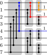
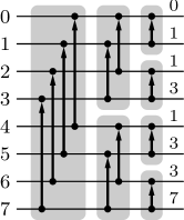
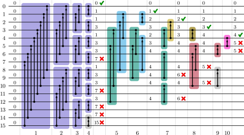
A pairwise sorting network starts with what we call a splitter cascade. That is, an initial splitter partitions the input wires into subsets of (roughly) equal size. Each subset is split recursively until wire singletons result (Zazon-Ivry & Codish, 2012). An example of such a splitter cascade is shown in Figure 4 for 8 wires and in purple color for 16 wires in Figure 5 (arrows point to where the larger value is desired).
After a splitter cascade, the value carried by wire has a minimum rank of , where counts the number of set bits in the binary number representation of . This minimum rank results from the transitivity of the swap operations in the splitter cascade, as is illustrated in Figure 4 for 8 wires: By following upward paths (in splitters to the left) through the splitter cascade, one can find for each wire exactly wires with smaller indices that must carry values no less than the value carried by wire . This yields the minimum ranks shown in Figure 4 on the right.
The core idea of our selection network construction is to use splitter cascades to increase the minimum ranks of (the values carried by) wires. If such a minimum rank exceeds (or equals , since we work with zero-based ranks and hence are interested in ranks ), a wire can be discarded, since its value is certainly not among the top . On the other hand, if there is only one wire with minimum rank 0, the top 1 value has been determined. More generally, if all minimum ranks no greater than some value occur for one wire only, the top values have been determined.
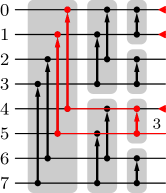
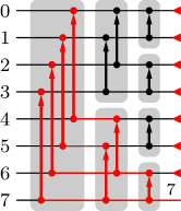
We exploit this as follows: Initially all wires are assigned a minimum rank of 0, since at the beginning we do not know anything about the values they carry. We then repeat the following construction: traversing the values descendingly, we collect for each all wires with minimum rank and apply a splitter cascade to them (provided there are at least two such wires). Suppose the wires collected for a minimum rank have indices . After the splitter cascade we can update the minimum rank of wire to , because before the splitter cascade there is no known relationship between wires with the same minimum rank, while the splitter cascade establishes relationships between them, increasing their ranks by . The procedure of traversing the minimum ranks descendingly, collecting wires with the same minimum rank and applying splitter cascades to them is repeated until all minimum ranks occur only once.
As an example, Figure 5 shows a selection network constructed is this manner, in which the minimum ranks of the wires are indicated after certain layers as well as when certain wires can be discarded (red crosses) and when certain top ranks are determined (green check marks). Comparators belonging to the same splitter cascade are shown in the same color.
| full | odd-even/pairwise/bitonic selection | splitter selection | |||||||||||||||
|---|---|---|---|---|---|---|---|---|---|---|---|---|---|---|---|---|---|
| sort | 1 | 2 | 3 | 4 | 5 | 6 | 7 | 8 | 1 | 2 | 3 | 4 | 5 | 6 | 7 | 8 | |
| 16 | 10 | 4 | 7 | 9 | 9 | 10 | 10 | 10 | 10 | 4 | 6 | 7 | 8 | 10 | 11 | 12 | 13 |
| 1024 | 55 | 10 | 19 | 27 | 27 | 34 | 34 | 34 | 34 | 10 | 14 | 16 | 18 | 22 | 25 | 27 | 29 |
| 10450 | 105 | 14 | 27 | 39 | 39 | 50 | 50 | 50 | 50 | 14 | 18 | 20 | 23 | 27 | 30 | 32 | 34 |
| 65536 | 136 | 16 | 31 | 45 | 45 | 58 | 58 | 58 | 58 | 16 | 20 | 22 | 25 | 29 | 32 | 34 | 36 |
While selection networks resulting from adaptations of sorting networks (see above) have the advantage that they guarantee that their number of layers is never greater than that of a full sorting network, our approach may produce networks with more layers. However, if is sufficiently small compared to (in particular, if ), our approach can produce selection networks with considerably fewer layers, as is demonstrated in Table 7. Since in the context we consider here we can expect , splitter-based selection networks are often superior.