Differential algebra of polytopes and inversion formulas

The following natural question goes back at least to Lagrange. For a given power series $\alpha(u)=u+\sum_{n\geq 1}a_{n}u^{n+1}$ find the inversion $\beta(v)$ under the substitution: $\alpha(\beta(v))\equiv v,\,\,\beta(\alpha(u))\equiv u.$ The coefficients of such series $\beta(v)=v+\sum_{n\geq 1}b_{n}v^{n+1}$ are known to be certain polynomials with integer coefficients:

$$b_{1}=-a_{1},\,b_{2}=-a_{2}+2a_{1}^{2},\,\,b_{3}=-a_{3}+5a_{1}a_{2}-5a_{1}^{3},$$

$$b_{4}=-a_{4}+6a_{1}a_{3}+3a_{2}^{2}-21a_{1}^{2}a_{2}+14a_{1}^{4}.$$

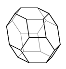
Remarkably these coefficients can be interpreted in terms of the combinatorics of the associahedra (or, Stasheff polytopes), see [5, 41] for the details. For example, the formula for $b_{4}$ says that $3D$ associahedron has 6 pentagonal and 3 quadrilateral faces, 21 edges and 14 vertices (see Fig. 1, where we show also its realisation as a truncated cube following [14]).

It is difficult to trace who was the first to observe this remarkable fact. The first combinatorial description of the coefficients $b_{n}$ seems to belong to Raney [53]. Stanley [56] provided 3 proofs in terms of tree combinatorics, known to be closely related to the associahedron. Loday [41] described this explicitly in terms of the associahedra, see also recent book by Aguiar and Ardila [5], who used the theory of Hopf monoids to derive this connection.

The aim of this paper is to provide one more derivation of this link using the differential equations for the generating function of the associahedra derived by one of the authors [11]. This allows us also to prove another known remarkable formula, expressing the multiplicative inversion of a formal power series in terms of combinatorics of permutohedra (see [5]) and to provide an interpretation of the combinatorics of cyclohedra in relation with the classical Faà di Bruno’s formula, which was first discovered by Aguiar and Bastidas [4]. In the case of the stellohedra we derive the relation with permutohedra, which seems to be new.

We discuss also the link with the rich theory of Deligne-Mumford moduli spaces $\bar{M}_{g,n}$, which are known to be related to associahedra [36], inversion formulas [44] and to the KdV hierarchy [60].

We start with a brief description of the differential algebra of simple polytopes following [11, 15]. For the general theory of convex polyhedra we refer to Ziegler [61].

Let $\mathfrak{P}:=\sum_{n\geq 0}\mathfrak{P}^{n}$ be the free abelian group generated by all convex polytopes, considered up to combinatorial equivalence and naturally graded by the dimension of the polytopes. The product of polytopes turns $\mathfrak{P}$ into a graded commutative ring with the unit given by the point, considered as $0$-dimensional polytope. Simple polytopes form a graded subring $\mathfrak{S}\subset\mathfrak{P}.$ Note that the ring $\mathfrak{P}$ is different both from the polytope algebra [46] of convex polytopes in $\mathbb{R}^{n}$ with product given by the Minkowski sum and from the Grothendieck ring of $\Gamma$-rational polytopes considered in [48].

A polytope is called indecomposable if it cannot be represented as a product of polytopes of positive dimension.

The proof can be found in [13] (see also Prop.1.7.2 in [15]). Note that if we introduce the second grading in $\mathfrak{P}$ by the number of the facets of polytopes, then the number of generators in any bi-graded component of $\mathfrak{P}$ will be finite [15].

Following [11] introduce the derivation $d$ in $\mathfrak{P}$ by defining the boundary $dP$ of a given polytope $P$ simply as the sum of all facets of $P$ considered as elements in $\mathfrak{P}$. It is easy to check that $d$ preserves the subring $\mathfrak{S}\subset\mathfrak{P}$ and satisfies the Leibnitz identity in $\mathfrak{P}$

$$d(P_{1}P_{2})=(dP_{1})P_{2}+P_{1}(dP_{2}).$$

This supplies $\mathfrak{P}$ with a structure of the differential ring, with $\mathfrak{S}$ being its differential subring. Note that in our case $d^{2}\neq 0$ in contrast with the differential introduced in [29].

We will be interested in the special class of simple polytopes known as graph-associahedra. They were introduced and studied in the work of Carr and Devadoss [20] and independently by Toledano Laredo [59] under the name De Concini–Procesi associahedra (see also Postnikov [51]). This class contains the classical series of permutohedra and associahedra.

Let $\Gamma$ be a connected simple (no loops or multiple edges) graph with the set of $n$ vertices, which we identify with $[n]:=\{1,2,\dots,n\}.$ The corresponding graph-associahedron $P_{\Gamma}$ is a particular case of the nestohedron [27] with the building set $\mathcal{B}=\mathcal{B}(\Gamma)$ consisting of the connected induced subgraphs of $\Gamma$, or equivalently as the subsets $S\subset[n]$ such that the restriction $\Gamma|_{S}$ is connected. Explicitly $P_{\Gamma}$ can be realised as the following $(n-1)$-dimensional convex polytope

(1)

$$P_{\Gamma}=\{x\in\mathbb{R}^{n}:\sum_{i=1}^{n}x_{i}=3^{n},\,\,\sum_{i\in S}x_{i}\geq 3^{|S|},\,S\in\mathcal{B},\,S\neq[n]\},$$

where $|S|$ is the number of elements in $S$ (see [59]).

The boundary of the graph-associahedra can be given by the following formula (see e.g. [15], Prop. 1.7.16). For any connected induced subgraph $S$ of $\Gamma$ with vertex set $[S]\subset[n]$ define the graph $\Gamma/S$ with the vertex set $[n]\setminus[S]$ having an edge between two vertices $i$ and $j$ whenever they are path-connected in the restriction $\Gamma|_{S\cup\{i,j\}}.$ Then the boundary of the graph-associahedron $P_{\Gamma}$ can be given combinatorially as

(2)

$$dP_{\Gamma}=\sum_{S\in\mathcal{B}(\Gamma),\,S\neq\Gamma}P_{S}\times P_{\Gamma/S}.$$

There are two famous particular cases of graph-associahedra: associahedra $\mathfrak{a}_{n}$ (or Stasheff polytopes, traditionally denoted as $K_{n+1}$) and permutohedra $\pi_{n}$, corresponding to path and complete graphs with $n$ vertices respectively.

For the associahedron $\mathfrak{a}_{n}$ the corresponding graph $\Gamma$ is a path with edges $(k,k+1),\,1\leq k\leq n$. The connected subgraphs $S$ are strings $[i,j]=(i,i+1,\dots,j-1,j)$, which can be naturally labelled by the brackets in the product $x_{1}x_{2}\dots x_{i-1}(x_{i}\dots x_{j})x_{j+1}\dots x_{n+1}$, linking this with the original Stasheff’s description (see [49, 61] for the history of this remarkable polytope and its role in combinatorics and algebra). The number of vertices of $\mathfrak{a}_{n}$ is the Catalan number $C_{n}=\frac{1}{n+1}{2n\choose n}.$ One can also describe $\mathfrak{a}_{n}$ also as the Newton polytope of the polynomial $\prod_{1\leq i<j\leq n}(x_{i}+x_{i+1}+\dots+x_{j-1}+x_{j}).$ For $n=3$ we have pentagon, for $n=4$ 3D associahedron, which is shown on Fig. 1 together with its realisation as 2-truncated cube found in [14].

Permutohedron $\pi_{n}$ corresponds to the complete graph with $n$ vertices and can be described as the convex hull of the points $\sigma(\rho)\in\mathbb{R}^{n},\,\sigma\in S_{n}$ with $\rho=(1,2,\dots,n),$ or as the Newton polytope of the Vandermonde polynomial $\prod_{1\leq i<j\leq n}(x_{i}-x_{j}).$ For $n=3$ we have hexagon, for $n=4$ - the truncated octahedron shown on Fig. 2.

Our first observation is that these two sequences of combinatorial polytopes can be characterised in terms of the differential algebra of polytopes as follows.

Let $P_{k},\,k\geq 0$ be a sequence of simple polytopes with the dimension of $P_{k}$ equal to $k.$ Consider the following question: when the corresponding subring of $\mathfrak{S}$ generated by these polytopes is closed under differentiation $d$ (and thus is a differential subring of $\mathfrak{S}$)?

Assuming that $P_{k}=P_{\Gamma_{k+1}}$ are graph-associahedra of the connected graphs $\Gamma_{k+1}$ with $k+1$ vertices, we can give the following answer.

We start with the differential equations for the generating functions of some special polytopes, derived by one of the authors [11] (see also [10] and [15], section 1.8).

Let $P$ be a convex polytope of dimension $n$ and $\mathcal{F}_{k}(P)$ be the set of all faces of $P$ of codimension $k$ considered as elements of $\mathfrak{P}$. Consider the corresponding generating function $F_{P}(t)\in\mathfrak{P}[t]$ defined by

(3)

$$F_{P}(t)=\sum_{k=0}^{n}t^{k}\sum_{f\in\mathcal{F}_{k}(P)}f=\sum_{f\in\mathcal{F}(P)}f\,t^{\text{codim}f}.$$

One can check that the valuation map $F_{t_{0}}:\mathfrak{P}\to\mathfrak{P}$ sending $P$ to $F_{P}(t_{0})$ is a ring-homomorphism for all $t_{0}$.

Define now the motivic interior $P^{\circ}$ of a polytope $P$ as the alternating sum of all the faces of $P:$

(4)

$$P^{\circ}:=F_{P}(-1)=\sum_{f\in\mathcal{F}(P)}(-1)^{\text{codim}f}f\in\mathfrak{P}.$$

At the level of the set-theoretical characteristic functions this formula agrees with a well-known result in the theory of finitely additive measures of convex polytopes [45, 52] with $P^{\circ}=relint(P)$ being the standard relative interior [61] of the polytope $P$. Note that the polytope $P$ can be represented simply as

$$P=\sqcup_{f\in\mathcal{F}(P)}relint(f),$$

where $\sqcup$ denotes the disjoint union of sets (see [61]). More justification for the terminology is given by the theory of toric varieties, see Section 5 below.

For simple polytopes we have the following formula, which will be important for us.

The proof easily follows from the simplicity of the polytope. In particular, for simple polytope $P$ the motivic interior can be written as $P^{\circ}=e^{-d}P.$

Following [11], consider now the generating functions of $F_{P}(t)$ for the families of associahedra and permutohedra

(6)		$\displaystyle\mathcal{A}(t,x):=\sum_{n=1}^{\infty}F_{\mathfrak{a}_{n}}(t)x^{n+1}=\mathfrak{a}_{1}x^{2}+(\mathfrak{a}_{2}+2\mathfrak{a}_{1}t)x^{3}+(\mathfrak{a}_{3}+5\mathfrak{a}_{2}t+5\mathfrak{a}_{1}t^{2})x^{4}+\dots,$
		$\displaystyle\mathcal{P}(t,x):=\sum_{n=1}^{\infty}F_{\pi_{n}}(t)\frac{x^{n}}{n!}=\pi_{1}x+(\pi_{2}+2\pi_{1}t)\frac{x^{2}}{2!}+(\pi_{3}+6\pi_{2}t+6\pi_{1}t^{2})\frac{x^{3}}{3!}+\dots.$

Here both $\mathfrak{a}_{1}$ and $\pi_{1}$ are points and thus are units in the polytopal ring, but for our purposes we will keep track of them considering them as independent variables. In particular, we define the corresponding weighted motivic interiors as

(7)		$\displaystyle\mathfrak{a}_{n}^{\circ}:=F_{\mathfrak{a}_{n}}(-\mathfrak{a}_{1})=\sum_{f\in\mathcal{F}(\mathfrak{a}_{n})}(-\mathfrak{a}_{1})^{\text{codim}f}f,$
		$\displaystyle\pi_{n}^{\circ}:=F_{\pi_{n}}(-\pi_{1})=\sum_{f\in\mathcal{F}(\pi_{n})}(-\pi_{1})^{\text{codim}f}f.$

For example, for $n=3$ we have $\mathfrak{a}_{3}^{\circ}=\mathfrak{a}_{3}-5\mathfrak{a}_{2}\mathfrak{a}_{1}+5\mathfrak{a}_{1}^{3},\,\,\pi_{3}^{\circ}=\pi_{3}-6\pi_{2}\pi_{1}+6\pi_{1}^{3}.$ The corresponding motivic interiors (4) can be found from the weighted motivic interiors by setting $\mathfrak{a}_{1}=\pi_{1}=1.$

Denote by

$$u_{t}(t,x):=\frac{\partial}{\partial t}u(t,x),\,\,u_{x}(t,x):=\frac{\partial}{\partial x}u(t,x)$$

the corresponding partial derivatives of the function $u(t,x).$

Indeed, the boundary formula (2) in this particular case gives

(10)

$$d\mathfrak{a}_{n}=\sum_{i=1}^{n-1}(i+1)\mathfrak{a}_{i}\times\mathfrak{a}_{n-i},\quad d\pi_{n}=\sum_{i=1}^{n-1}{n\choose i}\pi_{i}\times\pi_{n-i},$$

which together with Lemma leads to the differential equations (8), (9).

The partial differential equation

(11)

$$u_{t}=uu_{x}$$

is called Hopf equation (or inviscid Burgers’ equation) and used as the simplest model to describe the breaking of waves phenomenon.

It is well-known that its solution $u(t,x)$ with initial value $u(0,x)=f(x)$ can be given implicitly by the formula

(12)

$$u=f(x+ut),$$

which can be easily checked directly. Applying this now for the equation (8), we have the identity

(13)

$$\mathcal{A}(\mathfrak{a}_{1}t,x)=A(x+\mathcal{A}(\mathfrak{a}_{1}t,x)t).$$

Substituting here $t=-1$ we see that the generating function

(14)

$$A^{\circ}(x):=\mathcal{A}(-\mathfrak{a}_{1},x)=\sum_{n=1}^{\infty}\mathfrak{a}^{\circ}_{n}x^{n+1}$$

satisfies the relation

(15)

$$A^{\circ}(x)=A(x-A^{\circ}(x)).$$

Consider the series $\xi=x-A^{\circ}(x)$, then

$$x=\xi+A^{\circ}(x)=\xi+A(\xi).$$

Thus we have proved the following theorem, which is an interpretation of the result of Loday [41] (see also [5]).

Note that since by Theorem 2.1 and Proposition 2.2 the associahedra are algebraically independent in $\mathfrak{P}$, this implies the following universal inversion formulae: the coefficients of the formal series $\alpha(x)=x+\sum_{n\geq 1}a_{n}x^{n+1}$ and its compositional inverse $\beta(x)=x+\sum_{n\geq 1}b_{n}x^{n+1}$ are related by the following formulae, expressing each other as certain polynomials with integer coefficients:

$$b_{1}=-a_{1},\quad b_{2}=-a_{2}+2a_{1}^{2},\quad b_{3}=-a_{3}+5a_{1}a_{2}-5a_{1}^{3},$$

$$b_{4}=-a_{4}+6a_{1}a_{3}+3a_{2}^{2}-21a_{1}^{2}a_{2}+14a_{1}^{4},$$

in agreement with the formulas for the weighted motivic interiors of the associahedra

$$\mathfrak{a}^{\circ}_{1}=\mathfrak{a}_{1},\mathfrak{a}^{\circ}_{2}=\mathfrak{a}_{2}-2\mathfrak{a}_{1}^{2},\quad\mathfrak{a}^{\circ}_{3}=\mathfrak{a}_{3}-5\mathfrak{a}_{1}\mathfrak{a}_{2}+5\mathfrak{a}_{1}^{3},$$

$$\mathfrak{a}^{\circ}_{4}=\mathfrak{a}_{4}-6\mathfrak{a}_{1}\mathfrak{a}_{3}-3\mathfrak{a}_{2}^{2}+21\mathfrak{a}_{1}^{2}\mathfrak{a}_{2}-14\mathfrak{a}_{1}^{4}.$$

Note that the faces of $\mathfrak{a}_{n}$ of codimension $d$ are in one-to-one correspondence with dissections of a based $(n+3)$-gon by $d$ non-intersecting diagonals (see [30, 25]). Alternatively, the faces of $\mathfrak{a}_{n}$ can be labelled by non-isomorphic planar rooted trees with $n+1$ leaves [23], which can be used to rewrite the inversion formulas in these terms (see [56]).

The corresponding polynomials can also be expressed in terms of the partial Bell polynomials $B_{n,k}$ (see e.g. [21], Section 3.8) or, more explicitly, as

(17)

$$b_{n}=\frac{1}{(n+1)!}\sum_{k_{1}+2k_{2}+\dots=n,\,k_{i}\geq 0}(-1)^{k}\frac{(n+k)!}{k_{1}!k_{2}!\dots}a_{1}^{k_{1}}a_{2}^{k_{2}}\dots,$$

where $k=k_{1}+k_{2}+\dots$ (see e.g. [31]).

Similarly, the corresponding permutohedral differential equation (9) has the explicit solution

(18)

$$\mathcal{P}(\pi_{1}t,x)=\frac{\pi(x)}{1-t\pi(x)}.$$

Substituting here $t=-1$ we have the relation $\mathcal{P}(-\pi_{1},x)=\frac{\pi(x)}{1+\pi(x)}.$ This implies that $1-\mathcal{P}(-\pi_{1},x)=\frac{1}{1+\pi(x)}$ and the following result, which is an interpretation of the known result from [5].

Again since permotohedra are algebraically independent in $\mathfrak{P},$ this implies the universal multiplicative inversion formulae for the formal power series. Namely, the coefficients of the series $p(x)=1+\sum_{n=1}^{\infty}p_{n}\frac{x^{n}}{n!}$ and its multiplicative inverse $q(x)=1+\sum_{n=1}^{\infty}q_{n}\frac{x^{n}}{n!}$ are related by the polynomial formulas with integer coefficients: $q_{1}=-p_{1},\,q_{2}=-p_{2}+2p_{1}^{2},$

$$q_{3}=-p_{3}+6p_{1}p_{2}-6p_{1}^{3},\,\,\,q_{4}=-p_{4}+8p_{1}p_{3}+6p_{2}^{2}-36p_{1}^{2}p_{2}+24p_{1}^{4},$$

in agreement with the fact that $\pi_{3}$ is hexagon and $\pi_{4}$ has 8 hexagonal and 6 quadrilateral faces, 36 edges and 24 vertices (see Fig. 2). This is also in a good agreement with the formulas for the weighted motivic interiors of the permutohedra: $\pi^{\circ}_{1}=-p_{1},\,\pi^{\circ}_{2}=-p_{2}+2p_{1}^{2},$

(20)

$$\pi^{\circ}_{3}=\pi_{3}-6\pi_{1}\pi_{2}+6\pi_{1}^{3},\,\,\,\pi^{\circ}_{4}=\pi_{4}-8\pi_{1}\pi_{3}-6\pi_{2}^{2}+36\pi_{1}^{2}\pi_{2}-24\pi_{1}^{4}.$$

There is an interesting link with the moduli space $\bar{M}_{n}=\bar{M}_{0,n}$ of stable genus zero curves with $n$ ordered marked points. Its real version $\bar{M}_{n+1}(\mathbb{R})$ is known to be tessellated by $n!/2$ copies of associahedron $K_{n}$ (see [36, 23]). This explains the result of McMullen, who interpreted the compositional inversion formulas in terms of the corresponding real strata [44].

It is interesting that the geometry of the complex version $\bar{M}_{n+1}=\bar{M}_{n+1}(\mathbb{C})$ allows also to describe the compositional inversion of the exponential power series. More precisely, McMullen proved that the compositional inverse of the formal series $f(x)=x-\sum_{n\geq 1}a_{n}\frac{x^{n+1}}{(n+1)!}$ is given by

(21)

$$g(x)=x+\sum_{n\geq 1}b_{n}\frac{x^{n+1}}{(n+1)!},\quad b_{n}=\sum N_{n_{1},\dots,n_{s}}a_{n_{1}}\dots a_{n_{s}},$$

where $N_{n_{1},\dots,n_{s}}$ is the number of strata $S\subset\bar{M}_{n}(\mathbb{C})$ isomorphic to

$$M_{n_{1}}(\mathbb{C})\times\dots\times M_{n_{s}}(\mathbb{C})$$

(see Theorem 1 in [44]). The proof is based on the well-known bijection between the strata and the marked stable rooted trees, known also as modular graphs [40].

One can combine this with our result [16] claiming that the generating functions of the cobordism classes of the complex projective spaces $\mathbb{C}P^{n}$ and the theta-divisors $\Theta^{n}$

$$\alpha(z)=z+\sum_{n=1}^{\infty}[\mathbb{C}P^{n}]\frac{z^{n+1}}{n+1},\quad\beta(z)=z+\sum_{n=1}^{\infty}[\Theta^{n}]\frac{z^{n+1}}{(n+1)!},$$

are compositionally inverse to each other, to express the cobordism class $[\Theta^{n-1}]$ in terms of the cobordism classes $[\mathbb{C}P^{k}],\,k\leq n-1$ as follows

(22)

$$[\Theta^{n}]=\sum N_{n_{1},\dots,n_{s}}a_{n_{1}}\dots a_{n_{s}},\quad a_{k}=-k![\mathbb{C}P^{k}].$$

One more remarkable fact here is due to Getzler [32]. Recall that $\bar{M}_{n}$ is a special (Deligne-Mumford) compactification of the moduli space $M_{n}$ of $n$ ordered distinct points on complex projective line considered up to projective equivalence. Using the framework of the operads, Getzler proved that the exponential generating functions of the corresponding (in case of $M_{n}$, motivic) Poincare polynomials

$$F(t,x):=x-\sum_{n\geq 2}P_{M_{n+1}}(t)\frac{x^{n}}{n!},\quad G(t,y):=y+\sum_{n\geq 2}P_{\bar{M}_{n+1}}(t)\frac{y^{n}}{n!}$$

are inverse to each other: $F(G(t,y),t)\equiv y,\,\,G(F(t,x),t)\equiv x.$ Since the motivic Poincare polynomial

(23)

$$P_{M_{n}}(t)=(t^{2}-2)(t^{2}-3)\dots(t^{2}-n+2)$$

is known explicitly (see e.g. [37]), this determines $P_{\bar{M}_{n}}(t).$ Substituting here $t=-1$ we have the same relation between exponential generating functions of the Euler characteristics

$$F(x):=x-\sum_{n\geq 2}\chi(M_{n+1})\frac{x^{n}}{n!},\quad G(y):=y+\sum_{n\geq 2}\chi(\bar{M}_{n+1})\frac{y^{n}}{n!}.$$

Since $\chi(M_{n+1})=(-1)^{n}(n-2)!$ we see that $G(y)$ is the compositional inverse of the series $F(x)=x-\sum_{n\geq 2}\frac{(-1)^{n}}{n(n-1)}x^{n},$ which allows to compute $\chi(\bar{M}_{n}),$ giving OEIS sequence A074059: $2,\,7,\,34,\,213,\,1630,\,14747,\,153946,\,1821473...$

It is interesting that for the real version of Deligne-Mumford spaces $\bar{M}_{n}(\mathbb{R})$ McMullen proved that the same relation

$$B_{n}=\sum N_{n_{1},\dots,n_{s}}A_{n_{1}}\dots A_{n_{s}}$$

describes the functional inversion $G(x)=x-\sum_{n\geq 1}B_{n}x^{n+1}$ of the usual power series $F(x)=x+\sum_{n\geq 1}A_{n}x^{n+1}$ (see Corollary 5 in [44]).

Over finite fields one can interpret these results within the approach of Weil and Deligne as follows.

Let $\mathbb{F}_{p}$ with $p$ prime be the finite field with $p$ elements and $M_{0,n}(\mathbb{F}_{p}),\overline{M_{0,n}(\mathbb{F}_{p})}$ be the corresponding varieties over $\mathbb{F}_{p}.$ Let $|M_{0,n}(\mathbb{F}_{p})|$ and $|\overline{M_{0,n}(\mathbb{F}_{p})}|$ be the number of points in these varieties respectively.

The permutohedral variety $X_{\Pi}^{n}$ is the toric variety [22], corresponding to the $n$-dimensional permutohedron $\pi_{n+1}$. In particular, $X_{\Pi}^{1}=\mathbb{C}P^{1}$, $X_{\Pi}^{2}$ is the degree 6 del Pezzo surface.

Every toric variety $X^{n}$ is a closure of the algebraic torus $\mathbb{T}_{\mathbb{C}}^{n}=(\mathbb{C}^{*})^{n}$, which can be defined as the motivic interior of $X^{n}$.

To justify this consider the Grothendieck ring of complex quasi-projective varieties $K_{0}(\mathcal{V}_{\mathbb{C}})$ generated by the isomorphism classes of complex quasi-projective varieties modulo the relations

$$[X]=[Y]+[X\setminus Y],$$

where $Y$ is a Zariski locally closed subset of $X$, with multiplication given by the formula $[X]\textperiodcentered[Y]=[X\times Y]$ (see e.g. [33]).

Let $X_{P}$ be the smooth toric variety corresponding to a Delzant polytope $P$ and $Y_{f}\subset X_{P}$ be the toric subvariety corresponding to the face $f\in\mathcal{F}(P).$

The following result provides more justification for our definition of the motivic interior. In analogy with (4) define the motivic interior of $X_{P}$ as

(25)

$$[X_{P}^{\circ}]:=\sum_{f\in\mathcal{F}(P)}(-1)^{\text{codim}f}[Y_{f}]\in K_{0}(\mathcal{V}_{\mathcal{C}}).$$

The proof follows from the Proposition-definition 6 in [52] reformulated in terms of toric geometry [22] (see also Theorem 3.2.4 in [48]).

Note that similar relation holds for all convex polytopes if we extend it to the framework of the toric topology [15].

This implies that Theorem 3.5 can be reformulated as follows.

Motivic Poincare polynomial $P_{Z}(t),\,Z\in K_{0}(\mathcal{V}_{\mathbb{C}})$ defines the ring homomorphism $K_{0}(\mathcal{V}_{\mathbb{C}})\to\mathbb{Z}[t],$ where for the projective varieties $X,Y\subseteq X$ by definition

$$P_{[X\setminus Y]}(t)=P_{X}(t)-P_{Y}(t),$$

where $P_{X}(t)$ is the usual Poincare polynomial. In particular, since $\mathbb{C}^{*}$ is the complement of two points in $\mathbb{C}P^{1}$, the motivic Poincare polynomial $P_{[\mathbb{C}^{*}]}(t)=P_{\mathbb{C}P^{1}}(t)-2=(t^{2}+1)-2=t^{2}-1,$ and thus

$$P_{\mathbb{T}_{\mathbb{C}}^{n}}(t)=(t^{2}-1)^{n}.$$

As a corollary we have the following well-known fact (see e.g. [50]) relating permutohedral varieties with the classical Eulerian polynomials [19]. These polynomials were introduced by Euler in 1755 by the relation

$$\sum_{k=1}^{\infty}k^{n}t^{n}=\frac{tA_{n}(t)}{(1-t)^{n+1}}.$$

They have the generating function

(28)

$$\sum_{n\geq 0}A_{n}(s)\frac{x^{n}}{n!}=\frac{s-1}{s-e^{(s-1)x}}$$

and can be computed recursively by

$$A_{n+1}(t)=[t(1-t)\frac{d}{dt}+nt+1]A_{n}(t),\quad A_{0}=A_{1}=1:$$

$$A_{1}=1,\,\,A_{2}=s+1,\,\,A_{3}=s^{2}+4s+1,\,\,A_{4}=s^{3}+11s^{2}+11s+1,$$

$$A_{5}=s^{4}+26s^{3}+66s^{2}+26s+1,\,\,A_{6}=s^{5}+57s^{4}+302s^{3}+302s^{2}+57s+1.$$

Their coefficients are known as Eulerian numbers and have natural combinatorial interpretations (see [56]).

References

- [1] V.E. Adler On the combinatorics of several integrable hierarchies. J. Phys. A 48 (26) (2015), 265203.
- [2] V.E. Adler Set partitions and integrable hierarchies. Theor. Math.Physics 187:3 (2016), 842-870.
- [3] N. Amburg, E. Kreines, G. Shabat Poincare polynomial for the moduli space and the number of points in Moscow Univ. Math. Bull., 72 (2017),154-160.
- [4] M. Aguiar, J. Bastidas Associahedra, cyclohedra and inversion of power series. arXiv:2010.14283 (2020).
- [5] M. Aguiar, F. Ardila Hopf Monoids and Generalized Permutahedra. Memoirs of the AMS. Vol. 289, N.1437. AMS, 2023. arXiv:1709.07504 (2017).
- [6] P. Appell Sur une classe de polynômes. Annales Sci. École Norm. Supér. 2e Sèrie. 9 (1880), 119-144.
- [7] H. Bateman and A. Erdélyi Higher Transcendental Functions. Vol.III. McGraw-Hill Book Company, 1955.
- [8] R.P. Boas, R.C. Buck Polynomial expansion of analytic functions. Springer, 1958.
- [9] R. Bott and C. Taubes On the self-linking of knots. Journal of Math. Physics 35(10) (1994), 5247-5287.
- [10] V. M. Buchstaber, E. V. Koritskaya The quasi-linear Burgers-Hopf equation and the Stasheff polytopes. Funct. Anal. Appl. 41:3 (2007), 196-207.
- [11] V.M. Buchstaber Ring of simple polyhedra and differential equations. Trudy MIAN 263 (2008), 18-43.
- [12] V.M. Buchstaber, A.N. Kholodov Boas-Buck structures on sequences of polynomials. Funct. Anal. Appl. 23:4 (1989), 266-276.
- [13] V.M. Buchstaber, N. Erokhovets. Polytopes, Fibonacci numbers, Hopf algebras, and quasi-symmetric functions. Russian Math. Surveys 66 (2011), no. 2, 271-367.
- [14] V. M. Buchstaber, V. D. Volodin Combinatorial 2-truncated cubes and applications. Progress in Mathematics, 299 (2012), Birkhäuser, Basel, 161-186.
- [15] V.M. Buchstaber, T.E. Panov Toric Topology. Mathematical Surveys and Monographs, 204, AMS, 2015.
- [16] V.M. Buchstaber, A.P. Veselov Chern-Dold character in complex cobordisms and theta divisors. Advances in Math. 449 (2024), 109720, 1-35.
- [17] V.M. Buchstaber, A.P. Veselov Theta divisors and permutohedra. arXiv:2211.16042.
- [18] V.M. Buchstaber, S. Tersic̀ Moduli space of weighted pointed stable curves and toric topology of Grassmann manifolds. arXiv:2410.01059.
- [19] L. Carlitz Eulerian numbers and polynomials. Mathematics Magazine 32:5 (1959), 247-260.
- [20] M.P. Carr and S.L. Devadoss Coxeter complexes and graph-associahedra. Topology Appl. 153 (2006), no. 12, 2155-2168.
- [21] L. Comtet Advanced Combinatorics. D. Reidel Publ. Comp., Dordrecht, 1974.
- [22] D.A. Cox, J.B. Little, and H.K. Schenck Toric Varieties. Graduate Studies in Mathematics, vol. 124, American Mathematical Society, Providence, RI, 2011.
- [23] S.L. Devadoss Tesselations of moduli spaces and the mosaic operad. Contemp. Math. 239 (1999), 91–114.
- [24] S.L. Devadoss Space of cyclohedra. Discrete and Comput. Geometry 29 (2002), 61-75.
- [25] S.L. Devadoss and R.C. Read Cellular structures determined by polygons and trees. Annals of Combinatorics, 5 (2001), 71–98.
- [26] G. Falqui, C. Reina and A. Zampa Krichever maps, Faà di Bruno polynomials, and cohomology in KP theory. Lett. Math. Phys. 42 (1997), 349-361.
- [27] E.M. Feichtner and B. Sturmfels Matroid polytopes, nested sets and Bergman fans. Port. Math. (N.S.) 62 (2005), no. 4, 437-468.
- [28] A. Frabetti, D. Manchon Five interpretations of Faà di Bruno’s formula. arXiv:1402.5551 (2014).
- [29] A.A. Gaifullin Local formulae for combinatorial Pontrjagin classes. Izvestiya: Mathematics 68:5 (2004), 861-910.
- [30] I. M. Gelfand, M. M. Kapranov, and A. V. Zelevinsky Discriminants, Resultants, and Multidimensional Determinants. Birkhäuser Boston Inc., Boston, MA, 1994.
- [31] I.M. Gessel Lagrange inversion. J. Comb. Theory, Series A 144 (2016), 212-249.
- [32] E. Getzler Operads and moduli spaces of genus 0 Riemann surfaces. Progress in Math. 129 (1995), Birkhäuser Boston, Boston, MA,199-230.
- [33] S. M. Gusein-Zade, I. Luengo and A. Melle-Hernández A power structure over the Grothendieck ring of varieties. Math. Res. Lett. 11 (2004), 49-57.
- [34] A.J.J. Heidrich On the Factorization of Eulerian Polynomials. J. Number Theory 18 (1984), 157-168.
- [35] W.P. Johnson The curious history of Faà di Bruno’s formula. Amer. Math. Monthly 109:3 (2002), 217-234.
- [36] M.M. Kapranov The permutoassociahedron, Mac Lane’s coherence theorem and asymptotic zones for the KZ equation. J. Pure Appl. Algebra 85 (1993), no. 2, 119–142.
- [37] M.E. Kazaryan, S.K. Lando and V.V. Prasolov Algebraic Curves: Towards Moduli Spaces. Springer, 2019.
- [38] M. Kontsevich Feynman diagrams and low-dimensional topology. Progr. Math. 120 (1994), 97-121.
- [39] F. Lambert, J. Springael Soliton equations and simple combinatorics. Acta Appl. Math. 102 (2008), 147-178.
- [40] S.K. Lando, A.K. Zvonkin Graphs on Surfaces and Their Applications. Encyclopaedia of Mathematical Sciences, 141, Berlin, New York: Springer-Verlag, 2004.
- [41] J.-L. Loday The multiple faces of the associahedron. Clay Mathematics Institute Publication, 2005.
- [42] A. Losev and Y. Manin New moduli spaces of pointed curves and pencils of flat connec- tions. Michigan Math. J. 48 (2000), 443-472.
- [43] M. Markl Simplex, associahedron, and cyclohedron. Contemp. Math. 227, Amer. Math. Soc., Providence, RI, 1999.
- [44] C.T. McMullen Moduli spaces in genus zero and inversion of power series. L’Enseign. Math. (2) 60 (2014), 25–30.
- [45] P. McMullen Valuations and Euler-type relations on certain classes of convex polytopes. Proc. London Math. Soc. 35 (1977), 113-130.
- [46] P. McMullen The polytope algebra. Adv. Math. 78 (1989), 76-130.
- [47] Y. Mvondo-She From Hurwitz numbers to Feynman diagrams: Counting rooted trees in log gravity. Nuclear Physics B 995 (2023), 116350.
- [48] J. Nicaise Grothendieck rings of polytopes and non-archimedean semi-algebraic sets. arXiv:2402.11699.
- [49] V. Pilaud, F. Santos, G.M. Ziegler Celebrating Loday’s associahedron. Arch. Math. 121 (2023), 559–601.
- [50] A. Postnikov, V. Reiner, L. Williams Faces of generalized permutohedra. Doc. Math. 13 (2008), 207-273.
- [51] A. Postnikov Permutohedra, associahedra, and beyond. IMRN, 2009 (6), 1026-1106.
- [52] A.V. Pukhlikov, A.G. Khovanski Finitely additive measures of virtual polytopes. St. Petersburg Math. J. 4 (1993), no. 2, 337-356.
- [53] G.N. Raney Functional composition patterns and power series reversion. Trans. Amer. Math. Soc. 94 (1960), 441-451.
- [54] A.B. Shabat, M.Kh. Efendiev On applications of Faà-di-Bruno formula. Ufa Math. Journal 9:3 (2017), 131-136.
- [55] R. Simion A type-B associahedron. Advances in Applied Math. 30 (2003), 2-25.
- [56] R.P. Stanley Enumerative Combinatorics. Vol. 2. Cambridge University Press, 1999.
- [57] J. Stasheff Homotopy associativity of -spaces. I, II. Trans. Amer. Math. Soc. 108 (1963), 275–312.
- [58] J. D. Stasheff The pre-history of operads. Contemp. Math. 202 (1997), 53-81.
- [59] V. Toledano Laredo Quasi-Coxeter algebras, Dynkin diagram cohomology, and quantum Weyl groups. Int. Math. Res. Pap. IMRP 2008, Article ID rpn009, 167 pp.
- [60] E. Witten Two-dimensional gravity and intersection theory on moduli space. Surveys Diff.Geom. 1 (1991), 243-310.
- [61] G.M. Ziegler Lectures on Polytopes. Springer-Verlag, New York, 1995.