Differential configurational entropy and the gravitational collapse of a kink

The configurational entropy (CE) quantifies information and its transmission rate across channels of communication. The CE computes the amount of information that is concealed in stochastic variables and has been successfully implemented to survey a plethora of random physical systems and to scrutinize and quantify their different and relevant properties. In this way entropy in statistical mechanics and information entropy are interrelated concepts [1]. Similar to the Gibbs entropy, which generalizes the Boltzmann entropy for microstates that are not equiprobable, information entropy expresses the alterations of arrangement and disorder immanent to a given physical system. Shannon’s information entropy quantifies how much information is necessary to describe the specific detailed microscopic configuration of a system, once the associated macrostate is considered. Also, the rate of compression of the information is addressed by Shannon’s formulation. The CE was at first presented by Gleiser and Stamatopolous as a quantity that compares exact soliton-type solutions to approximations of it, eliminating the degeneracy of equal-energy ansätze regarding models containing a scalar field [2]. Besides, other configurational information measures were proposed to evaluate information and shape complexity of physical systems appearing in field theories [3, 4]. Several non-linear scalar field models that include kinks, solitons, bounces, and bubbles were scrutinized from the point of view of the CE, characterizing first-order phase transitions. Ref. [2] was the first seminal result in the literature to demonstrate that the lower the energy of a trial scalar field estimating exact solutions in field theory, the lower its associated CE is. In this setup, the CE was shown to pick the best fit for scalar field solutions. Matter configurations, encompassing kinks, solitons, oscillons, and stellar distributions, have been studied from the point of view of the DCE, with important information about stability [4, 5]. Ref. [6] analyzed the CE profile throughout a second-order phase transition, with an approach to criticality resembling the scaling behavior underlying the Kolmogorov-type turbulence in fluid flows, emulating the important concept of informational turbulence [7]. When continuous physical systems are taken into account, for low limits of almost lossless data compression, the differential configurational entropy (DCE) is the most suitable measure of information entropy [3, 4]. It can be evaluated by taking any spatially-localized, $\ell^{2}$-norm integrable scalar field [2, 5]. Global critical points of the DCE comply with microstates that have maximal configurational stability, being thus the preferred state of occupation of the system under scrutiny. The DCE has been applied to the solution of a variety of relevant physical systems. Gauge/gravity dualities and phase transitions were successfully investigated with the tools of the DCE [8, 9, 10, 11, 12]. Also, the DCE provided new features of black holes in anti-de Sitter (AdS) space [13, 14]. The Hawking–Page first-order phase transition was shown to correspond to the DCE global critical point [15]. In this respect, although AdS black holes can share stable thermal equilibrium with radiation, they are not the preferred state below a certain critical temperature, when thermal AdS emerges as the prevalent contribution to the partition function in AdS/CFT [16]. The stability of compact stellar distributions was also addressed in Ref. [17], corresponding to global minima of the DCE computed from the star energy density. The DCE has been auspiciously employed to address the stability of spatially-localized configurations of scalar fields in several different physical contexts. The DCE was used to derive the Chandrasekhar critical density of stellar core remnants consisting of electron-degenerate matter in Ref. [18], of collapsed neutron cores of massive supergiant stars in Ref. [19], and of Bose–Einstein condensates of gravitons, in Ref. [20]. Also, stellar configurations composed by gravitons in AdS were perused from the point of view of the DCE, derived as solutions of Einstein–Hilbert gravity with a gauge field, backreacting to the spontaneous compactification [21]. The DCE was also investigated in other different phenomenological contexts, with relevant results [22, 23, 25, 26, 27, 24, 28, 29].

The unequivocal experimental detection of gravitational waves, which are emitted from coalescing binary systems of stars and black holes as well, has currently consisted of prominent directions in physics [30, 31]. In the strong gravitational field regime, gravity can be successfully described by the theory of general relativity and some relevant generalizations, which can be probed by current observations, mostly at eLISA and LIGO. The gravitational critical behavior has been thoroughly studied in several contexts, employing a variety of theoretical and computational methods [33, 32]. This universal phenomenon appears in a myriad of circumstances, in particular including the gravitational collapse of scalar fields in several types of spacetimes [34]. A case of relevance involves a spherically symmetric scalar field, in the strong gravitational field limit approaching collapse and subsequent black hole formation. The gravitational critical behavior becomes even more fascinating and relevant when a mass gap is present in the evolution of a scalar field kink [35], therefore revealing important features of the scalar field gravitational collapse. Kinks have been explored in various contexts, including new gravitational sectors [36, 37]. Ref. [34] addressed critical points of bifurcation, determining the ramification into either a mass gap or no mass gap. An efficient procedure to approach this theme is to assume the Einstein–Klein–Gordon coupled system of effective field equations, to look over the gravitational collapse and subsequent black hole formation and its dynamics. The Einstein–Klein–Gordon system, coupling gravity to a scalar field, implements a generalization of general relativity and can solve observed deviations. Some conditions may also circumvent the no-hair conjecture [38, 39]. With it in hand, the critical behavior of gravitational collapse can be better probed with data regarding coalescing binary stars and black hole binary systems [40], with their particular experimental signatures detected from the gravitational collapse into gravitational wave radiation. Several open problems, regarding the stability of the gravitational collapse of Einstein–Klein–Gordon solutions, can be addressed using the DCE apparatus. Here we consider the gravitational collapse of a kink as studied in Refs. [35, 41], to explore the DCE under full numerical spacetimes with nontrivial features, such as the critical behavior discovered by Choptuik [33]. We set initially two kinds of kinks; one close to the well-known Janis–Newman–Winicour static solution [42] with a cutoff of the singular region and another very far–from–equilibrium. The first exhibits the critical behavior with a mass gap [41], and the second always forms a black hole [35]. The idea is to use these two extreme situations to explore how the DCE catches up with these highly nonlinear dynamical processes for the gravitational collapse and try to establish once more its physical robustness, also corroborating to well-established results in the literature as well as prospecting new relevant features regarding phase transitions and the gravitational collapse.

This paper is organized as follows: Section II is devoted to studying the Einstein–Klein–Gordon field equations, stressing the (matter) fluid correspondence with the massless scalar field. For it, the Bondi–Sachs metric plays a prominent role in defining a Bondi frame, and the Bondi mass is addressed. In Section III, the energy density associated with the scalar field is constructed upon the spatially-localized scalar field, its Fourier transform, the modal fraction, and the DCE, are discussed. Some previous results for the critical behavior are summarized and we give some information about the used numerical solver and scripting. In Section IVtwo initial conditions for the considered evolutions are set, including globally perturbed static kinks and the far-from-equilibrium kink solutions. In Section V the results are analyzed and discussed, investigating the role of the DCE in determining a phase transition. It distinguishes two main types of evolution profiles into final equilibria, that can either lead to a final black hole state or a static solution. Ulterior features and analysis are reported, also in Section VI.

We consider the Einstein-Klein-Gordon equations of motion

	$\displaystyle G_{\mu\nu}$	$\displaystyle=$	$\displaystyle-8\pi T_{\mu\nu},$		(1a)
	$\displaystyle\square\Upphi$	$\displaystyle=$	$\displaystyle 0,$		(1b)

where $G_{\mu\nu}$ denotes the Einstein’s tensor

$$T^{\Upphi}_{\mu\nu}=\nabla_{\mu}\Upphi\nabla_{\nu}\Upphi-\frac{1}{2}g_{\mu\nu}\nabla^{\alpha}\Upphi\nabla_{\alpha}\Upphi.$$

(2)

Spherically symmetric solutions have an initial value setup that comprises outgoing null cones emerging out a central geodesic. For it, one denotes by $u$ the (proper) time coordinate along the geodesic, assuming constant values on the outgoing null cones. Therefore the Bondi–Sachs coordinates, $x^{\mu}=(u,r,\theta,\phi)$ can be employed to write the Bondi–Sachs metric under spherical symmetry [43]

$$ds^{2}=e^{2\beta}\left(\frac{V}{r}du^{2}+2dudr\right)-r^{2}(d\theta^{2}+\sin^{2}\theta d\phi^{2}),$$

(3)

It is worth mentioning that the normal covector field $k_{\mu}=\partial_{\mu}u$ is null, also implying that the corresponding future-pointing vector field $k^{\mu}=-g^{\mu\nu}\partial_{\nu}u$ is a tangent vector field along the null-ray manifold. When $r\to 0$, the conditions

	$\displaystyle V(u,r)$	$\displaystyle=$	$\displaystyle r+\mathcal{O}(r^{3}),$		(4a)
	$\displaystyle\beta(u,r)$	$\displaystyle=$	$\displaystyle\mathcal{O}(r^{2}),$		(4b)

must be imposed for the Minkowski spacetime be recovered.

The Misner–Sharp mass function, $\tilde{m}(u,r)$ [44] introduced by means of

$$\tilde{m}=\frac{1}{2}(r-Ve^{-2\beta}),$$

(5)

measures the energy content in the sphere of radius $r$ and it reduces to the Arnowitt–Deser–Misner and Bondi masses in the appropriate limits.

The energy-momentum tensor for the massless scalar field minimally coupled to gravity can be characterized as a radiating and anisotropic fluid [45, 46]

	$\displaystyle T^{\Upphi}_{\mu\nu}$	$\displaystyle=$	$\displaystyle(\rho^{\Upphi}+p_{t}^{\Upphi})u_{\mu}u_{\nu}+\varepsilon^{\Upphi}l_{\mu}l_{\nu}-p_{t}^{\Upphi}g_{\mu\nu}$		(6)
			$\displaystyle\qquad+(p^{\Upphi}_{r}-p_{t}^{\Upphi})\chi_{\mu}\chi_{\nu},$

with $u^{\mu}u_{\mu}=1,$ $l^{\mu}l_{\mu}=0,$ $\chi^{\mu}\chi_{\mu}=-1,$ when one identifies the 4-velocity for an observer at rest, with respect to the metric (3), by

$$u^{\mu}=\left(1-\frac{2\tilde{m}}{r}\right)^{-1/2}e^{-2\beta}\delta^{\alpha}_{0},$$

(7)

and the null and the space-like vectors respectively expressed as

	$\displaystyle l_{\mu}$	$\displaystyle=$	$\displaystyle\left(1-\frac{2\tilde{m}}{r}\right)^{1/2}e^{2\beta}\delta^{0}_{\mu},$		(8a)
	$\displaystyle\chi_{\mu}$	$\displaystyle=$	$\displaystyle\left(1-\frac{2\tilde{m}}{r}\right)^{-1/2}\delta^{1}_{\mu}.$		(8b)

The scalar energy flux, the scalar energy density, the scalar radial pressure, and the scalar tangential pressure, are respectively given by

	$\displaystyle\!\!\!\!\epsilon^{\Upphi}$	$\displaystyle=$	$\displaystyle e^{-2\beta}\left[e^{-2\beta}\left(1-\frac{2\tilde{m}}{r}\right)^{-1}(\Upphi_{,u})^{2}-\Upphi_{,u}\Upphi_{,r}\right],$		(9)
	$\displaystyle\!\!\!\!\rho^{\Upphi}$	$\displaystyle=$	$\displaystyle p^{\Upphi}_{r}=\frac{1}{2}\left(1-\frac{2\tilde{m}}{r}\right)(\Upphi_{,r})^{2},$		(10)
	$\displaystyle\!\!\!\!p_{t}^{\Upphi}$	$\displaystyle=$	$\displaystyle\Upphi_{,u}\Upphi_{,r}e^{-2\beta}-p_{r}^{\Upphi},$		(11)

where the comma denotes partial differentiation with respect to the indicated coordinate. Note that Bondian observers can be purely Lagrangian when we deal only with radiation. The observer with four-velocity (7) is resting at infinity [47].

The field equations (1a, 1b) reduce to the well known hypersurface equations for a scalar field [48, 35, 41]

	$\displaystyle\beta_{,r}=2\pi r(\Upphi_{,r})^{2},$		(12a)
	$\displaystyle V_{,r}=e^{2\beta},$		(12b)

whereas the Klein–Gordon equation can be expressed as and

$$2(r\Upphi)_{,ur}=r^{-1}[re^{2\beta}(r-2\tilde{m})\Upphi_{,r}]_{,r},$$

(13)

in Bondi coordinates. The initial null data that is necessary for analyzing the evolution of the system is given by $\Upphi(0,r)$, in the region exterior to $R$. Also, at this boundary the condition $\Upphi(u,R)=A=\;$constant is adopted, together with the gauge condition limit $\lim_{r\to\infty}\Upphi(u,r)=0$ and $\beta(u,R)=0$. Since the metric must match a flat inner region, $r<R$, then $V(u,R)=R$.

These constraints on the scalar field and the metric as well have therefore a unique evolution across the future. The outcome metric is not asymptotically Minkowski at the future null infinity, being specified by the function $H(u)=\lim_{r\to\infty}\beta(u,r)$, whose additional role is to correlate the Bondi time, $u_{\scriptscriptstyle{B}}$, at the future null infinity to the proper time by the following expression,

$$\frac{du_{\scriptscriptstyle{B}}}{du}=e^{2H(u)}.$$

(14)

The 4-tuple of coordinates $(u_{\scriptscriptstyle{B}},r,\theta,\phi$) comprise a Bondi frame with metric given by Eq. (3), as long as the concomitant mappings $V\mapsto V_{\scriptscriptstyle{B}}=e^{-2H}V$ and $\beta\mapsto\beta_{\scriptscriptstyle{B}}=\beta-H$ are implemented. Using the Bondi time is suitable to probe asymptotic quantities, whereas the proper time is appropriate to study event horizons [41]. The Bondi mass of the Einstein–Klein–Gordon system reads [48]

$\displaystyle M(u)$

$\displaystyle=$

$\displaystyle 2\pi\int_{R}^{\infty}e^{2H(u)-\beta(u,r)}r^{2}(\Upphi_{,r})^{2}\,dr,$

(15)

or, equivalently,

$\displaystyle M$

$\displaystyle=$

$\displaystyle 2\pi\int_{R}^{\infty}rVe^{-2\beta}(\Upphi_{,r})^{2}\,dr.$

(16)

To implement observational aspects of the results here to be presented, one can make an expansion of the scalar field $\Upphi$, near the future null infinity, as [51]

$$\phi(u,r)=\frac{c(u)}{r}+\frac{c_{\scriptscriptstyle\text{NP}}}{r^{2}}+O(r^{-3}),$$

(17)

where the coefficient $c_{\scriptscriptstyle\text{NP}}$ of the $1/r^{2}$-term in the expansion is the Newman–Penrose constant of the scalar field. Replacing Eq. (17) into the hypersurface equations yields

	$\displaystyle\!\!\!\!\!\!\!\!\!\!\!\beta(u,r)\!$	$\displaystyle\!=\!$	$\displaystyle\!H(u)-\frac{\pi c^{2}(u)}{r^{2}}+O(r^{-3}),$		(18)
	$\displaystyle\!\!\!\!\!\!\!\!\!\!\!V(u,r)\!$	$\displaystyle\!=\!$	$\displaystyle\!e^{2H(u)}\left(r\!-\!2M(u)\!+\!\frac{\pi c^{2}(u)}{r}\right)\!+\!O(r^{-2}),$		(19)

where $H(u)$ is given by Eq. (14). The Bondi mass-loss equation asserts that

$$\frac{dM}{du_{\scriptscriptstyle{B}}}=-4\pi\left(\frac{dc(u_{\scriptscriptstyle{B}})}{du_{\scriptscriptstyle{B}}}\right)^{2}.$$

(20)

One can therefore analyze radiation emission for near-critical evolution profiles. The monopole moment of the scalar field $c(u_{\scriptscriptstyle{B}})$ in (17) has usually a (damped) oscillation with a frequency that exponentially decreases. Also, half-periods in $c(u_{\scriptscriptstyle{B}})$ comply with the ones emerging from the slightest quasinormal mode of Schwarzschild-type solutions, with effective background mass $M_{1}(u_{\scriptscriptstyle{B}})$, obtained when one evaluates the Bondi mass at its inflection points. Perturbation fields outside black holes evanesce according to an inverse power-law tail, as a byproduct of late-time decay of radiative fields, and reflects the backscattering phenomenon of waves modes off the effective curvature potential. For late times, perturbation theory yields the field to fall off as $\Upphi\propto u_{\scriptscriptstyle{B}}^{-2}$, near the future null infinity, and $\Upphi\propto u_{\scriptscriptstyle{B}}^{-3}$, near the timelike infinity. One can consider an observer at constant $r$ and Bondi time $\Delta u_{\scriptscriptstyle{B}}$, elapsed when the emitted radiation pulse has been detected by the observer [51]. The null infinity can be estimated by the range $\Delta u_{\scriptscriptstyle{B}}\ll r$, defining the so-called astrophysical zone. Also, the convergence of the perturbation expansion requires $\Delta u_{\scriptscriptstyle{B}}\gg M_{1}$, whereas the mass associated with the effective potential has an upper bound ruled by the mass producing the initial ingoing pulse, $M_{\scalebox{0.66}{{init}}}$, where $\Delta u_{\scriptscriptstyle{B}}\gg M_{\scalebox{0.66}{{init}}}$. One may observe tails for $\Delta u_{\scriptscriptstyle{B}}\gtrsim 10^{3}M_{\scalebox{0.66}{{init}}}$.

Several relevant measures of information entropy have been implemented, mainly in the last decade, and utilized to study gravitational systems and quantum field theories. Among them, the configurational entropy (CE) and its differential version (DCE) play a prominent role in investigating several physical systems and determining their preferred occupied state, always corresponding to critical points of the CE and the DCE. The CE can be established, once one regards the original formulation of information entropy by Shannon [1], which defined information by the expression $S=-\sum_{c_{i}\in{\mathcal{C}}}p_{c_{i}}\log p_{c_{i}},$ where the sum is taken over the set $\mathcal{C}=\{c_{i}\}$, for $i=1,\ldots,N$, consisting of symbols, which have a respective probability distribution $p_{i}=p(c_{i})$ determining their occurrence. The amount of information contained by each symbol was determined by Shannon as $\mathbb{I}(c_{i})=-\log_{2}p_{i}$, and satisfies the expression [4]

$$\langle\mathbb{I}\rangle=\sum_{c_{i}\in\mathcal{C}}p(c_{i})\mathbb{I}(c_{i})=-\sum_{c_{i}\in\mathcal{C}}p(c_{i})\log_{2}p(c_{i})=S.$$

(21)

The precise concept of information regards the lowest number of bits that are needed to convert symbols into a coded form, in such a way that the highest transmission rate of messages, that consist of an array of the given symbols, can be achieved across some transmission channel. Therefore, $\log_{2}N$ is the number of bits to describe $N$ symbols. When one regards a uniform distribution, randomness is related to the probability distribution $p(c)=1/N$, whose entropy is the highest possible at $\langle\mathbb{I}\rangle=\log_{2}N$. The base of the logarithm to be used is a matter of choice, as the binary base 2 logarithm measures the information entropy in bits, whereas one can employ the natural logarithm corresponding to measuring the information entropy in the natural unit of entropy (nat or Sh [shannon]). One nat is equal to $1/\ln 2$ shannon $\approx$ 1.4427 Sh. There is a correlation involving the CE and the Gibbs entropy, ${S_{\scalebox{0.66}{{thermo}}}=-k_{{\mathsf{B}}}\sum_{a}p_{a}\ln p_{a}\,}$, for $k_{\mathsf{B}}$ denoting the Boltzmann constant, and $p_{i}$ stands for the probability of occurrence of each specific detailed microscopic configuration of the system. Thermodynamic systems have microstates that do not have necessarily equal probabilities. The Boltzmann equation, $S_{\scalebox{0.66}{{thermo}}}=k_{\mathsf{B}}\ln(\mathsf{W})$, where $\mathsf{W}$ is the number of equiprobable microstates, was generalized by the Gibbs entropy, for the case of microstates that are not equiprobable. The CE quantifies the entropy in the context of information, as entropy in thermodynamics is equivalent to the portion of information, in the Shannon’s sense, required for comprising microstates constituting a physical system [8]. The spectral Fourier transform of the energy density,

$${\scalebox{0.85}{{$\uprho$}}}(k)=\frac{1}{\sqrt{2\pi}}\int_{\mathbb{R}}e^{i{{k}}{\mathsf{r}}}\rho({\mathsf{r}})d\mathsf{r},$$

(22)

matches the collective coordinate concept in the statistical mechanics context, $\rho(r)\sim\sum e^{-ik_{n}r}{\scalebox{0.85}{{$\uprho$}}}(k_{n})$, when the limit of continuum mechanics is taken into account. The static structure factor is given by

$\displaystyle f(k_{n})=\frac{\left|{\scalebox{0.85}{{$\uprho$}}}(k_{n})\right|^{2}}{\sum_{a=1}^{n}\left|{\scalebox{0.85}{{$\uprho$}}}(k_{a})\right|^{2}},$

(23)

which measures the probability distribution of any field pattern of the propagating waves with wavenumber $k_{n}$.

Going to the continuum mechanical limit, one can consider the DCE, which measures the information related to the energy density with $\ell^{2}$-norm. The Fourier transform of the energy density yields the energy spectral density,

$\displaystyle{\scalebox{0.85}{{$\uprho$}}}({k})=\frac{1}{\sqrt{2\pi}}\int_{\mathbb{R}}{\scalebox{0.85}{{$\uprho$}}}({r})e^{-i{k}\cdot{r}}dr,$

(24)

and mimics collective coordinates in the continuum mechanical limit of statistical mechanics [8]. The relative weight of distinct wave modes is quantified by the modal fraction,

$\displaystyle\mathsf{f}_{\scalebox{0.6}{{$\uprho$}}}(k)=\frac{|{\scalebox{0.85}{{$\uprho$}}}({k})|^{2}}{\int_{\mathbb{R}}|{\scalebox{0.85}{{$\uprho$}}}({\mathsf{k}})|^{2}d\mathsf{k}}.$

(25)

The modal fraction measures the weight carried by the wave modes associated with the wavenumber $k$. The portion of the information that is necessary to set out the shape of the density, here describing the scalar field coupled to gravity, is computed by the DCE [5],

$\displaystyle S[{\scalebox{0.85}{{$\uprho$}}}]=-\int_{\mathbb{R}}\invbreve{\mathsf{f}}_{{\scalebox{0.6}{{$\uprho$}}}}({{\mathsf{k}}})\ln\left[\invbreve{\mathsf{f}}_{{\scalebox{0.6}{{$\uprho$}}}}({\mathsf{k}})\right]d\mathsf{k},$

(26)

where $\invbreve{\mathsf{f}}_{\scalebox{0.6}{{$\uprho$}}}({k})=\mathsf{f}_{\scalebox{0.6}{{$\uprho$}}}({k})/\mathsf{f}_{\scalebox{0.6}{{$\uprho$}}}^{\scalebox{0.52}{{max}}}({k})$, being $\mathsf{f}_{\scalebox{0.6}{{$\uprho$}}}^{\scalebox{0.52}{{max}}}({k})$ the maximal value of the modal fraction at the wavenumber whose power spectral density has a peak. The more the scalar field configuration is localized over the space, the more the configuration escalates across the momentum space. Consequently, the higher the DCE is. Still, the configurational stability of the physical system here scrutinized and its regarded DCE are contiguous correlated quantities. The system stability regards the global minimum of the DCE, analyzed about the parameter that regulates the physical features of the system.

The DCE and the Bondi mass will be now discussed with respect to the proper time and the Bondi time. The results of the computations are presented and discussed in what follows.

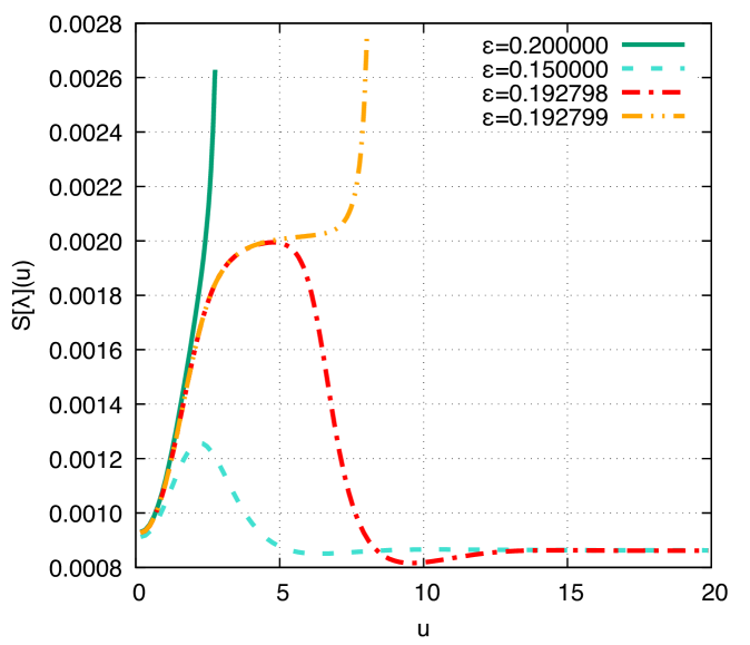
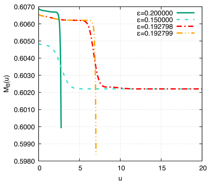
Fig. 1, the plot on top, shows the DCE as a function of the proper time for the stable kink I. The black hole formation is evident whenever the perturbation parameter $\varepsilon$ in Eq. (35) surpasses the critical value $\varepsilon_{\scalebox{0.66}{{crit${}_{1}$}}}\approxeq 0.1927985$, which determines a bifurcation point, wherefrom we can distinguish subcritical and supercritical evolution profiles. For subcritical evolution, regarding values of the perturbation parameter lower than $\varepsilon_{\scalebox{0.66}{{crit${}_{1}$}}}$, there is no black hole formation. In this way, the DCE exhibits a typical bifurcation for the critical gravitational collapse. In this case, with higher values of the proper time, the DCE converges to the asymptotic preferential value of the static solution recovering equilibria, since it lacks a black hole collapse process. This critical value of the DCE, corresponding a first-order phase transition, is invariant for all $\varepsilon<\varepsilon_{\scalebox{0.66}{{crit${}_{1}$}}}$. It is also worth emphasizing that for values $\varepsilon>\varepsilon_{\scalebox{0.66}{{crit${}_{1}$}}}$, corresponding to a supercritical evolution, the DCE is a monotonically increasing function of the proper time. The higher the value of the perturbation parameter $\varepsilon$ in Eq. (35), the higher the increment rate of the DCE with respect to the proper time is. In the range $\varepsilon<\varepsilon_{\scalebox{0.66}{{crit${}_{1}$}}}$ that characterizes subcritical solutions, the DCE has a peak for any fixed value of the perturbation parameter. The higher the value of $\varepsilon$, the more the proper time elapses to attain the peak of the DCE. In the range $\varepsilon<\varepsilon_{\scalebox{0.66}{{crit${}_{1}$}}}$, the system returns to the state of equilibrium, $\Upphi(\upalpha)$, at late proper times. Besides, every fixed value of the perturbation parameter in the range $\varepsilon<\varepsilon_{\scalebox{0.66}{{crit${}_{1}$}}}$ yields a global minimum of the DCE, corresponding to a transient plateau in the Bondi mass and to the maximum of the monopole, which decays up to a constant final value. The higher the value of $\varepsilon$ in this range, the more the proper time elapses to reach the respective minimum of the DCE and the lower the value of the minimum is. After the minimum, the DCE fastly converges to the asymptotic preferential value of the static solution. The location of global minima in different cases presents no scaling behavior.

Now, Fig. 1, the plot on the bottom, depicts the Bondi mass as a function of the proper time, for different values of the perturbation parameter $\varepsilon$ in Eq. (35). For the sake of consistency, the same values of the parameters in the plot on top are respectively employed. The first important feature regards the monotonicity of the Bondi mass with respect to the proper time. In the supercritical evolution range, the higher the value of the perturbation parameter $\varepsilon$, the steeper the Bondi mass decreases with respect to the proper time, up to the collapse process leading to black hole formation. The Bondi mass profile suddenly changes at $\varepsilon_{\scalebox{0.66}{{crit${}_{1}$}}}$ and in the subcritical evolution range the Bondi mass also converges to the asymptotic preferential value of the static solution for $\upalpha=1$, with no black hole formation. When $\upalpha=1$, the kink potential assumes $A_{\Upphi}(\upalpha)|_{\upalpha\to 1}=0.36563$. The Bondi mass approaches its asymptotic equilibrium value, $M_{\Upphi}(\upalpha)|_{\upalpha\to 1}\approxeq 0.60220$.

In Fig. 2 the unstable kink I is illustrated and analyzed. The upper plot depicts the DCE as a function of the proper time for the unstable kink I ($\upalpha=1.42429$). The black hole formation is again manifest whenever the perturbation parameter $\varepsilon$ in Eq. (35) reaches values that are higher than the critical value $\varepsilon_{\scalebox{0.66}{{crit${}_{2}$}}}\approxeq 3.42\times 10^{-7}$, which regulates a bifurcation point for the unstable kink I. Values $\varepsilon\gtrless\varepsilon_{\scalebox{0.66}{{crit${}_{2}$}}}$ respectively determine supercritical and subcritical evolution of the gravitational kink. Similarly to the stable kink I, the range $\varepsilon<\varepsilon_{\scalebox{0.66}{{crit${}_{2}$}}}$ yields no black hole formation. Also, the DCE converges to the asymptotic preferential value of the static solution that regards a first-order phase transition, being invariant for all $\varepsilon<\varepsilon_{\scalebox{0.66}{{crit${}_{2}$}}}$ in the subcritical evolution profile. Every fixed value of the perturbation parameter in the range $\varepsilon<\varepsilon_{\scalebox{0.66}{{crit${}_{2}$}}}$ yields a global minimum of the DCE. The lower the value of $\varepsilon$ in this range, the less the proper time elapses to reach the respective minimum of the DCE and the higher the value of the minimum is. After the minimum, the DCE rapidly converges to the asymptotic preferential value of the static solution for $\upalpha=1$. However, in the supercritical evolution range $\varepsilon>\varepsilon_{\scalebox{0.66}{{crit${}_{2}$}}}$, the DCE is a monotonically non-decreasing function of the proper time. The lower the value of $\varepsilon$ in Eq. (35), the lower the increment rate of the DCE, with respect to the proper time, is.

The plot on the bottom in Fig. 2 depicts the Bondi mass as a function of the proper time, for different values of the perturbation parameter $\varepsilon$. For the sake of consistency, the same values of the parameters in the plot on top in Fig. 2 are respectively employed. The Bondi mass is a monotonically non-increasing function of the proper time. In the supercritical evolution range, the higher the value of the perturbation parameter $\varepsilon$, the sharper the Bondi mass decreases, up to the collapse process leading to black hole formation. The Bondi mass profile is then modified at the bifurcation point defined by the critical value $\varepsilon_{\scalebox{0.66}{{crit${}_{2}$}}}$. In the subcritical evolution range, the Bondi mass also converges to the asymptotic preferential value of the static solution for $\upalpha=1$, when black holes are not formed.

Fig. 3 illustrates the DCE as a function of the Bondi time, for several kink I evolution profiles, including stable and unstable configurations. The critical, subcritical, and supercritical asymptotic values of the DCE are the same for evolution profiles in the respective channel. As expected, there is a subtle qualitative difference when comparing to the DCE, here as a function of the Bondi time, and in Fig. 1, as a function of the proper time, mainly in what concerns the supercritical evolution profile. Although being still a monotonically non-decreasing function of the Bondi time, the DCE at the supercritical evolution profile has a plateau at the preferential asymptotic value. There are also bifurcation points, from which subcritical and supercritical evolution profiles can be discerned. Yet the subcritical evolution points to no black hole origination, and the DCE evinces a typical bifurcation for the critical gravitational collapse. For higher values of the Bondi time, the DCE converges to the asymptotic preferential value of the static solution, for both the stable and unstable evolution profiles. The higher the value of the perturbation parameter, the higher the increment rate of the DCE with respect to the Bondi time is. Subcritical solutions present a peak of the DCE. The higher the value of the perturbation parameter, the more the Bondi time elapses to reach the peak of the DCE. Also, in the subcritical range, there are global minima of the DCE for each fixed value of the perturbation parameter. The lower the value of the perturbation parameter in the subcritical range, the less the proper time elapses to reach the respective global minimum of the DCE, and the higher the value of the global minimum is. For values of the Bondi time that are in the future when compared to the Bondi time regarding the global minima, the DCE fastly converges to the asymptotic preferential value of the static solution. In the subcritical range $\varepsilon<\varepsilon_{\scalebox{0.66}{{crit${}_{1}$}}}$, we numerically verified that for the DCE as a function of the Bondi time, the maximum value of DCE, denoted by $S_{\scalebox{0.52}{{peak}}}$, scales with $\varepsilon$ (see Fig. 3) as

	$\displaystyle\!\!\!\!\!\!\!\!\!S_{\scalebox{0.52}{{peak}}}(\varepsilon)$	$\displaystyle=$	$\displaystyle 13013.5038\varepsilon^{3}-6950.1781\varepsilon^{2}+1229.6481\varepsilon$		(37)
			$\displaystyle\qquad\qquad\qquad\qquad\quad\qquad\qquad-71.9875,$

within $0.01\%$ numerical error.

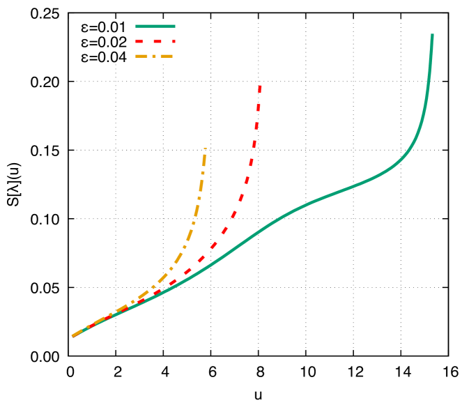
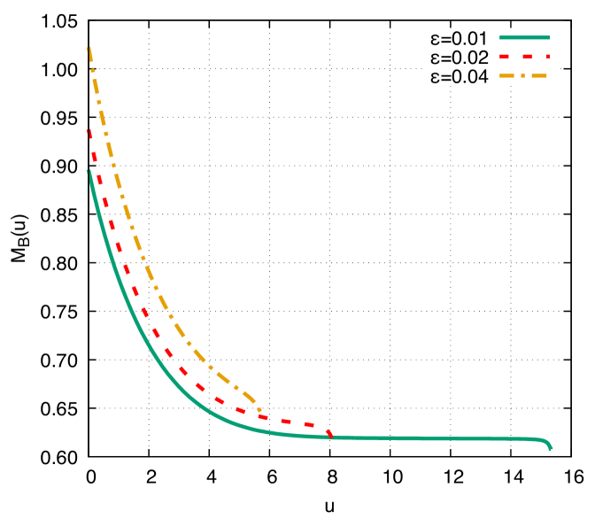
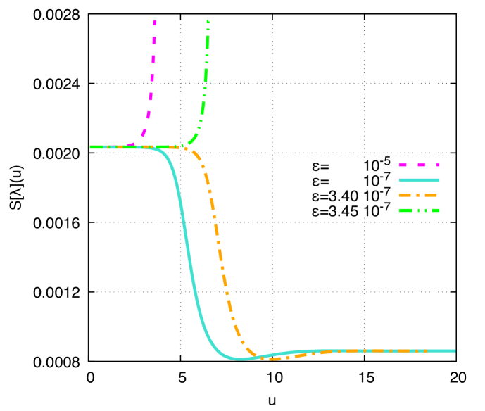
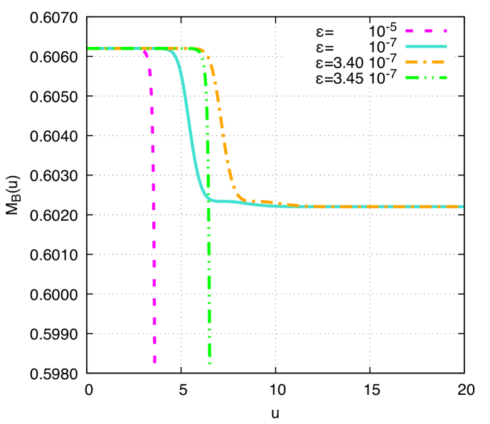
The plot on top in Fig. 4 refers to the DCE as a function of the proper time for the kink II. Irrespectively of the value of the perturbation parameter, the DCE is a monotonically increasing function of the proper time. For values $\varepsilon\gtrsim 0.015$, there is an interesting change of behavior of the DCE characterized by ${d^{2}S[\lambda](u)}/{du^{2}}>0$, for all values of the proper time. Still, for lower values of $\varepsilon$, ${d^{2}S[\lambda](u)}/{du^{2}}>0$ just for higher values of the proper time. It is worth emphasizing that the higher the value of the perturbation parameter $\varepsilon$, the steeper the increment rate of the DCE is, respectively with higher values of ${d^{2}S[\lambda](u)}/{du^{2}}$, accordingly. In all cases analyzed, the final state of the kink is the gravitational collapse, leading to black hole formation as the scalar field pours its associated hair. The Bondi mass is also presented as a function of the proper time for the kink II, in the plot on the bottom in Fig. 4. The Bondi mass is a monotonically decreasing function of the proper time, presenting ${d^{2}S[\lambda](u)}/{du^{2}}>0$ in almost all the ranges respectively illustrated, but an end-stage corresponding to a very short proper time interval, where the Bondi mass has a sudden decay to a final state. This attribute holds for any value of the perturbation parameter. The higher the value of the perturbation parameter, the shorter the proper time elapses for the Bondi mass to reach the end-stage.

The gravitational collapse of two types of kinks was heretofore investigated, employing the DCE setup. Globally perturbed static kinks, prospected here in both the stable and unstable cases, source two end-stage equilibria, consisting of either a static solution or the formation of the black hole near the scalar field critical collapse. This ramification, determined by a critical amplitude perturbation, categorizes a first-order phase transition containing a mass gap, wherein the black hole formation represents a supercritical domain, whereas static solutions regard the subcritical range, with no possibility of forming a black hole by the scalar field collapse. The DCE precisely designates the critical amplitude perturbation as a branching process governing the critical gravitational collapse, also emulating the respective supercritical and subcritical regions for the associated Bondi mass. In the subcritical case, both the Bondi mass and the DCE have been shown to converge, respectively, to the asymptotic preferential values of static solutions. For the far-from-equilibrium kink solutions, the DCE corroborates black hole formation from the gravitational collapse of the kink, for all cases of the critical amplitude perturbation. Regardless of the value of the perturbation parameter, the DCE was derived as a monotonically increasing function of the proper time, diverging at finite proper time elapse, leading to collapse into a black hole. On the other hand, the Bondi mass associated with far-from-equilibrium kinks always decreases with time. Black holes formed by the process here described and endorsed by DCE methods might exist as an observable physical by-product of the evolution of solutions of the Einstein–Klein–Gordon system. They may form coalescing black hole binary mergers emitting gravitational waves radiation, whose physical signatures can be predominantly probed with the gravitational wave detectors [52]. Their observational analysis may provide a groundbreaking source of information about the strong-field regime of general relativity. The analysis of Extreme Mass Ratio Inspirals can impart useful hints about Einstein–Klein–Gordon systems, since perturbative models of the inspiral sector record a noteworthy imprint of a scalar field on observable gravitational wave radiation [53]. It is worth mentioning that the leading-order influence arises from dipolar radiation emission, with a scalar field coupled to gravity. At the leading order, each black hole merger in the binary system emulates a monopole, whereas the binary system emits dipole radiation, also imposing bounds on massless scalar fields according to the latest binary pulsar observations [54]. Extreme mass-ratio inspirals onto supermassive black holes play a prominent role in the phenomenological aspects here studied, as scalar monopoles are accelerated by gravity at the supermassive black hole, emitting scalar radiation that comprises mostly of dipole radiation. The growing effect at the long-lasting inspiral can be detectable at ground-based detectors [30, 31], with additional energy loss, and subsequent dephasing of the gravitational waveform, depending on the scalar field as here proposed, dressing the supermassive black hole.

References

- [1] C. E. Shannon, Bell Syst. Tech. J. 27 (1948) 379.
- [2] M. Gleiser and N. Stamatopoulos, Phys. Lett. B 713 (2012) 304 [arXiv:1111.5597 [hep-th]].
- [3] M. Gleiser, M. Stephens and D. Sowinski, Phys. Rev. D 97 (2018) 096007 [arXiv:1803.08550 [hep-th]].
- [4] M. Gleiser and D. Sowinski, Phys. Rev. D 98 (2018) 056026 [arXiv:1807.07588 [hep-th]].
- [5] M. Gleiser and N. Stamatopoulos, Phys. Rev. D 86 (2012) 045004 [arXiv:1205.3061 [hep-th]].
- [6] M. Gleiser and D. Sowinski, Phys. Lett. B 747 (2015) 125 [arXiv:1501.06800 [cond-mat.stat-mech]].
- [7] D. Sowinski and M. Gleiser, J. Stat. Phys. 167 (2017) 1221 [arXiv:1606.09641 [cond-mat.stat-mech]].
- [8] A. E. Bernardini and R. da Rocha, Phys. Lett. B 762 (2016) 107 [arXiv:1605.00294 [hep-th]].
- [9] N. R. F. Braga and R. da Rocha, Phys. Lett. B 776 (2018) 78 [arXiv:1710.07383 [hep-th]].
- [10] N. R. F. Braga, R. da Mata, Phys. Lett. B 811 (2018) 135918 Phys. Lett. B 811 (2020) 135918 [arXiv:2008.10457 [hep-th]].
- [11] N. R. Braga and R. da Mata, Phys. Rev. D 101 (2020) 105016 [arXiv:2002.09413 [hep-th]].
- [12] N. R. F. Braga and O. C. Junqueira, Phys. Lett. B 814 (2021) 136082 [arXiv:2010.00714 [hep-th]].
- [13] N. R. F. Braga, Phys. Lett. B 797 (2019) 134919 [arXiv:1907.05756 [hep-th]].
- [14] C. O. Lee, Phys. Lett. B 772 (2017) 471 [arXiv:1705.09047 [gr-qc]].
- [15] N. R. F. Braga and R. da Rocha, Phys. Lett. B 767 (2017) 386 [arXiv:1612.03289 [hep-th]].
- [16] C. O. Lee, Phys. Lett. B 824 (2022) 136851 [arXiv:2111.04111 [hep-th]].
- [17] A. Fernandes-Silva, A. J. Ferreira-Martins, R. da Rocha, Phys. Lett. B 791 (2019) 323 [arXiv:1901.07492 [hep-th]].
- [18] M. Gleiser and D. Sowinski, Phys. Lett. B 727 (2013) 272 [arXiv:1307.0530 [hep-th]].
- [19] M. Gleiser and N. Jiang, Phys. Rev. D 92 (2015) 044046 [arXiv:1506.05722 [gr-qc]].
- [20] R. Casadio and R. da Rocha, Phys. Lett. B 763 (2016) 434 [arXiv:1610.01572 [hep-th]].
- [21] R. da Rocha, Phys. Lett. B 823 (2021) 136729 [arXiv:2108.13484 [gr-qc]].
- [22] G. Karapetyan, Phys. Lett. B 786 (2018) 418 [arXiv:1807.04540 [nucl-th]].
- [23] G. Karapetyan, Phys. Lett. B 781 (2018) 205 [arXiv:1802.09105 [nucl-th]].
- [24] R. A. C. Correa, D. M. Dantas, C. A. S. Almeida, R. da Rocha, Phys. Lett. B 755 (2016) 358 [arXiv:1601.00076 [hep-th]].
- [25] D. Bazeia, D. C. Moreira and E. I. B. Rodrigues, J. Magn. Magn. Mater. 475 (2019) 734 [1812.04950 [cond-mat.mes-hall]].
- [26] R. A. C. Correa, R. da Rocha and A. de Souza Dutra, Annals Phys. 359 (2015) 198 [arXiv:1501.02000 [hep-th]].
- [27] D. Bazeia and E. I. B. Rodrigues, Phys. Lett. A 392 (2021) 127170.
- [28] W. T. Cruz, D. M. Dantas, R. V. Maluf and C. A. S. Almeida, Annalen Phys. 531 (2019) 1970035.
- [29] F. C. E. Lima and C. A. S. Almeida, Eur. Phys. J. C 81 (2021) 1044 [arXiv:2111.07403 [hep-th]].
- [30] B. P. Abbott et al. [LIGO Scientific and Virgo], Phys. Rev. Lett. 119 (2017) 161101 [arXiv:1710.05832 [gr-qc]].
- [31] Y. Q. Xue, X. C. Zheng, Y. Li, W. N. Brandt, B. Zhang, B. Luo, B. B. Zhang, F. E. Bauer, H. Sun and B. D. Lehmer, et al. Nature 568 (2019) 198 [arXiv:1904.05368 [astro-ph.HE]].
- [32] W. Barreto, H. P. de Oliveira and B. Rodriguez-Mueller, Gen. Rel. Grav. 49 (2017) 107 [arXiv:1707.04938 [gr-qc]].
- [33] M. Choptuik, Phys. Rev. Lett. 70 (1993) 9.
- [34] D. Santos-Oliván and C. F. Sopuerta, Phys. Rev. Lett. 116 (2016) 041101 [arXiv:1511.04344 [gr-qc]].
- [35] W. Barreto, R. Gómez, L. Lehner, J. Winicour, Phys. Rev. D 54 (1996) 3834 [arXiv:gr-qc/0507086].
- [36] D. Bazeia, A. S. Lobao, Jr. and R. Menezes, Phys. Rev. D 86 (2012) 125021 [arXiv:1210.6874 [hep-th]].
- [37] D. Bazeia, L. Losano, M. A. Marques and R. Menezes, Phys. Lett. B 736 (2014) 515 [arXiv:1407.3478 [hep-th]].
- [38] J. Ovalle, R. Casadio, E. Contreras, A. Sotomayor, Phys. Dark Univ. 31 (2021) 100744 [arXiv:2006.06735 [gr-qc]].
- [39] J. Ovalle, E. Contreras and Z. Stuchlik, Phys. Rev. D 103 (2021) 084016 [arXiv:2104.06359 [gr-qc]].
- [40] F. Pretorius, Phys. Rev. Lett. 95 (2005) 121101 [arXiv:gr-qc/0507014 [gr-qc]].
- [41] W. Barreto, J. Crespo, H. de Oliveira, E. Rodrigues, B. Rodriguez-Mueller, Phys. Rev. D 93 (2016) 064042 [arXiv:1603.00852 [gr-qc]].
- [42] A. Janis, E. T. Newman, and J. Winicour, Phys. Rev. Lett. 20 (1968) 878.
- [43] H. Bondi, Proc. R. Soc. London A 281 (1964) 39.
- [44] C. W. Misner, D. H. Sharp, Phys. Rev. 136 (1964) 571.
- [45] L. Herrera and N. O. Santos, Phys. Rep. 286 (1997) 53.
- [46] W. Barreto, L. Castillo and E. Barrios, Phys. Rev. D 80 (2009) 084007 [arXiv:0909.4500 [gr-qc]].
- [47] L. Herrera, W. Barreto, J. Carot, A. Di Prisco, Class. Quant. Grav. 24 (2007) 2645 [arXiv:gr-qc/0703125 [gr-qc]].
- [48] R. Gómez, J. Winicour, J. Math. Phys. 33 (1992) 1445.
- [49] R. Gómez, J. Winicour, and R. Isaacson, J. Comput. Phys. 98 (1992) 11.
- [50] W. Barreto, Phys. Rev. D 89 (2014) 084071 [arXiv:1404.4016 [gr-qc]].
- [51] M. Pürrer, S. Husa and P. C. Aichelburg, Phys. Rev. D 71 (2005) 104005 [arXiv:gr-qc/0411078 [gr-qc]].
- [52] J. G. Baker, J. Centrella, D. I. Choi, M. Koppitz and J. van Meter, Phys. Rev. Lett. 96 (2006) 111102 [arXiv:gr-qc/0511103 [gr-qc]].
- [53] A. Maselli, N. Franchini, L. Gualtieri, T. P. Sotiriou, Phys. Rev. Lett. 125 (2020) 141101 [arXiv:2004.11895 [gr-qc]].
- [54] P. C. C. Freire, N. Wex, G. Esposito-Farese, J. P. W. Verbiest, M. Bailes, B. A. Jacoby, M. Kramer, I. H. Stairs, J. Antoniadis and G. H. Janssen, Mon. Not. Roy. Astron. Soc. 423 (2012) 3328 [arXiv:1205.1450 [astro-ph.GA]].