Differential cumulants, hierarchical models and monomial ideals

This paper draws together three areas: a new concept of differential cumulants, hierarchical models and the theory of monomial ideals in algebra. The central idea is that for a strictly positive density $f_{X}(x)$ of a $p$-dimensional random vector $X$, the mixed partial derivative of the log density $g_{X}(x)=\log f_{X}(x)$ can be used to express independence and conditional independence statements. Thus, for random variables $X_{1},X_{2},X_{3}\text{ in }\mathbb{R}$, the condition

$$\frac{\partial^{2}}{\partial x_{1}\partial x_{2}}g_{X_{1},X_{2},X_{3}}(x_{1},x_{2},x_{3})=0\text{ for all }(x_{1},x_{2},x_{3})\text{ in }\mathbb{R}^{3}$$

(1)

is equivalent to the conditional independence statement

$$X_{1}\mathchoice{\mathrel{\hbox to0.0pt{$\displaystyle\perp$\hss}\mkern 2.0mu{\displaystyle\perp}}}{\mathrel{\hbox to0.0pt{$\textstyle\perp$\hss}\mkern 2.0mu{\textstyle\perp}}}{\mathrel{\hbox to0.0pt{$\scriptstyle\perp$\hss}\mkern 2.0mu{\scriptstyle\perp}}}{\mathrel{\hbox to0.0pt{$\scriptscriptstyle\perp$\hss}\mkern 2.0mu{\scriptscriptstyle\perp}}}X_{2}|X_{3}.$$

In the next section we show how such mixed partial derivatives can be interpreted as differential cumulants. Then, in section 3, we show how collections of differential equations like (1) can be used to express independence and conditional independence models. Section 4 shows that, more generally, these collections can be used to define hierarchical statistical models of exponential form.

Section 5 maps the hierarchical model conditions to monomial ideals, which are increasingly being used within algebraic statistics. This isomorphism maps, for example, the mixed partial derivative condition (1) to the monomial ideal $<x_{1}x_{2}>$ within the polynomial ring $k[x_{1},x_{2},x_{3}]$. The equivalence allows ideal properties to be interpreted as hierarchical model properties, opening up an algebraic-statistical interface with some potential.

This section can be considered as a development from a body of work on local correlation. Good examples are the papers of Holland & Wang (1987), Jones (1996) and Bairamov et al. (2003). We draw particularly on Mueller & Yan (2001).

Let $X\in\mathbb{R}^{p}$ be a random vector. We assume $X$ has a $p+1$ times continuously differentiable density $f_{X}$. Once we introduce the concept of differential cumulants, we further require $f_{X}$ be strictly positive.

For $x,k\text{ in }\mathbb{R}^{p}$ we set $x^{k}\mathrel{\mathop{\ordinarycolon}}=\prod_{i=1}^{p}x_{i}^{k_{i}},\;x!\mathrel{\mathop{\ordinarycolon}}=\prod_{i=1}^{p}x_{i}!$ and $m_{k}=\mathbb{E}(X^{k}).$ Let $M_{X}\mathrel{\mathop{\ordinarycolon}}\mathbb{R}^{p}\longrightarrow\mathbb{R}$ and $K_{X}\mathrel{\mathop{\ordinarycolon}}\mathbb{R}^{p}\longrightarrow\mathbb{R}$ denote the moment and cumulant generating functions of $X$ respectively. For a vector $k\text{ in }\mathbb{N}^{p}$ we set

$$D^{k}f(x)\mathrel{\mathop{\ordinarycolon}}=\frac{\partial^{\,\mathinner{\!\left\lVert k\right\rVert}_{1}}}{\prod_{i=1}^{p}\partial x_{i}^{k_{i}}}f(x),$$

where $\mathinner{\!\left\lVert k\right\rVert}_{1}\mathrel{\mathop{\ordinarycolon}}=\sum_{i=1}^{p}\mathinner{\!\left\lvert k_{i}\right\rvert}$ is the Manhattan norm. By convention $D^{0}f(x)\mathrel{\mathop{\ordinarycolon}}=f(x)$.

The cumulant $\kappa_{k}$ can be found by evaluating $D^{k}(\log(M_{X}(t))$ at zero. We use the multivariate chain rule (given e.g. in Hardy, 2006) stated in Theorem 1. At the heart of the chain rule is an identification of differential operators with multisets:

Associated with a partition $\pi$ of a multiset $M$ is a combinatorial quantity to which we refer as the collapse number $c(\pi)$. It is defined as

$$c(\pi)\mathrel{\mathop{\ordinarycolon}}=\frac{\nu_{M}!}{\prod_{i\in I}\nu_{M_{i}}!\nu_{\pi}!}.$$

See Hardy (2006) for a combinatorial interpretation of $c(\pi)$.

The expression for cumulants in terms of moments is particularly simple in what we shall call the square-free case, that is for cumulants $\kappa_{k}$, whose index vector $k$ is binary. In that case, the multiset associated with $k$ is degenerate and $c(\pi)=1$. Equation (2) simplifies to

$$\kappa_{k}=\sum_{\pi\in\Pi(k)}(-1)^{(\mathinner{\!\left\lvert\pi\right\rvert}-1)}(\mathinner{\!\left\lvert\pi\right\rvert}-1)!\prod_{j=1}^{p}m_{\nu_{M_{j}}}.$$

In this form it is often stated and derived via the classical Faa Di Bruno formula applied to an exponential function followed by a Moebius inversion (see e.g. Barndorff-Nielsen & Cox, 1989).

Local analogues to moments and cumulants can be derived as one considers their limiting counterparts in the neighborhood of a fixed point $\xi\text{ in }\mathbb{R}^{p}$, an idea proposed by Mueller & Yan (2001). This section derives formulae for local moments and cumulants and local moment generating functions provided its global counterpart exists.

For a strictly positive edge length $\epsilon\text{ in }\mathbb{R}_{+}$, let $A(a,\epsilon)\mathrel{\mathop{\ordinarycolon}}=[\xi-\frac{\epsilon}{2},\xi+\frac{\epsilon}{2}]^{p}$ denote the hyper cube centralized at $\xi$. Let $\mathinner{\!\left\lvert A\right\rvert}=\epsilon^{p}$ denote its volume. The density of the random variable $X\text{ in }\mathbb{R}^{p}$ conditional on being in $A$ is given by

$$f^{A}_{X}(x)=\frac{f_{X}(x)1\hskip-7.39772pt{1}_{A}(x)}{pr(X\in A)},$$

where $1\hskip-7.39772pt{1}_{A}(x)$ is the indicator function which returns unity if $x$ is in $A$ and zero otherwise. The conditional moments about $\xi$ are denoted by

$$m^{A}_{k}=\mathbb{E}\bigg{(}\prod_{i=1}^{p}(X_{i}-\xi_{i})^{k_{i}}\mathinner{\Bigr{\rvert}}X\in A\bigg{)}.$$

Let $2\mathbb{N}$ and $2\mathbb{N}\hskip-3.0pt+\hskip-3.0pt1$ denote the set of positive even and odd integers respectively. For symmetry reasons, even and odd orders of individual components have different effects on local moments, which motivates the following definition:

$$\mathinner{\!\left\lVert\alpha\right\rVert}^{+}_{1}\mathrel{\mathop{\ordinarycolon}}=\mathinner{\!\left\lVert\alpha\right\rVert}_{1}+\sum_{i=1}^{p}1\hskip-7.39772pt{1}\;(\alpha_{i}\in 2\mathbb{N}\hskip-1.0pt+\hskip-1.0pt1).$$

$\mathinner{\!\left\lVert\cdot\right\rVert}^{+}_{1}$ increments the total sum of the components of a vector by one additional unit for each odd component (it is not to be interpreted as a norm).

A natural way to extend the concept of a local moment is to consider the limiting case when $\epsilon\rightarrow 0$. This leads to our definition of differential moments.

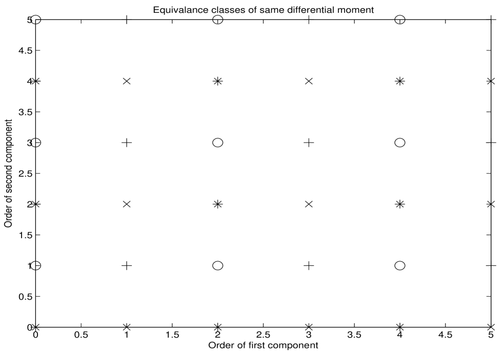
From (3) it is clear that the choice of $\alpha$ in the derivative $D^{\alpha}f_{X}$ depends only on the pattern of odd and even components of the moment. To be precise, $\alpha$ holds a unity corresponding to odd components and a zero corresponding to even component entries. Consequently, the differential moment $m^{\xi}_{k}$ depends on $k$ only via the pattern of odd and even values.

This suggests defining an equivalence relation on $\mathbb{N}^{p}\times\mathbb{N}^{p}$: For $u,k\in\mathbb{N}^{p}$ set $u\sim_{m}k\iff m_{u_{1}\cdots u_{p}}=m_{k_{1}\cdots k_{p}}$. The relation $\sim_{m}$ partitions the product space $\mathbb{N}^{p}\times\mathbb{N}^{p}$ into $2^{p}$ equivalence classes of same differential moments. The graph corresponding to $\sim_{m}$ is depicted in Figure 1 for the bivariate case. The axes give the order of the moment for the two components. Different symbols represent different equivalence classes. For instance, $(2,2)\sim_{m}(4,2)$, since $m^{\xi}_{22}=m^{\xi}_{42}$. Note that $u\sim_{m}k\iff\mathinner{\!\left\lVert u-k\right\rVert}_{1}\in 2\mathbb{N}$.

Similarly to local moments, for any measurable set $A$ we can define a local moment generating function:

$$M_{X}^{A}(t)\mathrel{\mathop{\ordinarycolon}}=\mathbb{E}(e^{t^{\prime}X}|X\in A).$$

Being a conditional expectation, it exists if $M_{X}$ exists. We have the following expansion:

	$\displaystyle M^{A}_{X}(t)$	$\displaystyle=\frac{1}{pr(X\in A)}\int_{A}e^{\sum_{i=1}^{p}t_{i}x_{i}}f_{X}(x)dx$
		$\displaystyle=1+\sum_{i=1}^{p}t_{i}\mathinner{\frac{\partial f_{X}(x)}{\partial x_{i}}\Biggr{\rvert}}_{x=\xi}\bigg{(}\frac{\epsilon^{2}}{3f_{X}(\xi)}+O(\epsilon^{4})\bigg{)}$
		$\displaystyle+\sum_{i=1}^{p}t_{i}^{2}\mathinner{\frac{\partial^{2}f_{X}(x)}{\partial x_{i}^{2}}\Biggr{\rvert}}_{x=\xi}\bigg{(}\frac{\epsilon^{2}}{6f_{X}(\xi)}+O(\epsilon^{4})\bigg{)}$
		$\displaystyle+\sum_{i=1}^{p}\sum_{j>i}^{p}t_{i}t_{j}\mathinner{\frac{\partial^{2}f_{X}(x)}{\partial x_{i}\partial x_{j}}\Biggr{\rvert}}_{x=\xi}\bigg{(}\frac{\epsilon^{4}}{9f_{X}(\xi)}+O(\epsilon^{6})\bigg{)}+O(\epsilon^{4}\mathinner{\!\left\lVert t^{3}\right\rVert}).$

The local moments can be computed from the local moment generating function via differentiation to appropriate order and evaluation at $t=0$. The natural logarithm of the local moment generating function defines the local cumulant generating function $K^{A}_{X}(t)\mathrel{\mathop{\ordinarycolon}}\mathbb{R}^{p}\longrightarrow\mathbb{R}$:

$$K^{A}_{X}(t)\mathrel{\mathop{\ordinarycolon}}=\log(M^{A}_{X}(t)).$$

Similarly to differential moments we can define differential cumulants at $\xi$. Two different ways of doing so are natural. First, taking the limiting quantity of the local cumulants as $\epsilon\rightarrow 0$ or, second, taking the series of differential moments and requiring that the mapping between moments and cumulants is preserved which is induced through the ex-log relation of the associated generating functions, see also the discussion in (McCullagh, 1987, page 62).

As demonstrated below, the two quantities just described differ in general and coincide only in the square-free case. In order to retain the intuitive and familiar relation between cumulants and moments, we define differential cumulants in terms of differential moments.

We are now in a position to state the main result of this section, namely that mixed partial derivatives of the log density can be interpreted as differential cumulants.

This is a multivariate generalization of the local dependence function introduced by Holland & Wang (1987). The next theorem relates differential cumulants to the limit of local cumulants.

Of particular interest to us are differential cumulants which vanish everywhere. We refer to them as zero-cumulants. Writing $g=\log f_{X}$, we shall usually write $D^{\alpha}g=0$ to denote the zero-cumulant associated with $\alpha$ in the understanding that this holds for all $x$.

The next section shows that sets of zero cumulants are isomorphic to conditional independence statements. As a consequence of lemma 1 zero-cumulants are invariant under diagonal transformations of the random vector $X$. In particular, they are not affected by the probability integral transformation and hence any result below holds also true for the copula density of $X$.

From now on, we shall assume that $f_{X}$ is strictly positive everywhere. Sets of zero-cumulants are equivalent to conditional and unconditional dependency structures.

In the multivariate case, we can express conditional independence of any pair given the remaining variables through square free differential cumulants.

Setting several square-free differential cumulants to zero simultaneously allows us to express conditional independence statements.

Pairwise conditional independence of all pairs is equivalent to independence.

The analysis of the last section makes clear that setting certain mixed two-way partial derivatives of $g(x)=\log f_{X}(x)$ equal to zero, is equivalent to independence or conditional independence statements. We can go further and define a generalized hierarchical model using the same process.

The basic structure of a hierarchical model can be define via a simplicial complex. Thus let $\mathcal{N}=\{1,\ldots,p\}$ be the vertex set representing the random variables $X_{1},...,X_{p}$. A collection $\mathcal{S}$ of index sets $J\subseteq\mathcal{N}$ is a simplicial complex if it is closed under taking subsets, i.e. if $J\text{ in }\mathcal{S}$ and $K\subseteq J$ then $K\text{ in }\mathcal{S}$.

This is equivalent to a quasi-additive model for $g(x)=\sum_{J\in\mathcal{S}}h_{J}(x_{J}),$ and we also refer to this model for $g(x)$ as being hierarchical. It is clear that we may write the model over the maximal cliques only, namely simplexes which are not contained in a larger simplex. In the terminology of Lauritzen (1996) we require $f_{X}$ be positive and factorise according to $\mathcal{S}$ for it to be a hierarchical model with respect to $\mathcal{S}$.

Associated to an index set $K\subseteq\mathcal{N}$ is a differential operator $D^{k}$, where $k=\sum_{i\in K}e_{i}\in\{0,1\}^{p}$ holds ones for every member of $K$ and zeros otherwise. In the following, we overload the differential operator by allowing it to be superscripted by a set or by a vector. Thus, for an index set $K$ we set $D^{K}\mathrel{\mathop{\ordinarycolon}}=D^{k}$ and similarly $\kappa_{K}^{x}\mathrel{\mathop{\ordinarycolon}}=\kappa_{k}^{x}$. $D^{K}$ returns the differential cumulant $\kappa_{K}^{x}$, when applied to $g(x)$.

We collect the results of the last section into a comprehensive statement. First, we define the complementary complex to a simplicial complex $\mathcal{S}$ on $\mathcal{N}$.

Note immediately that $\bar{\mathcal{S}}$ is closed under unions, i.e. $K,K^{\prime}\text{ in }\bar{\mathcal{S}}\Rightarrow K\cup K^{\prime}\in\bar{\mathcal{S}}$. It is a main point of this paper that there is a duality between setting collections of mixed differential cumulants equal to zero and a general hierarchical model:

The growing area of algebraic statistics makes use of computational commutative algebra particularly for discrete probability model, notably Poisson and multinomial log-linear models. Work connecting the algebraic methods to continuous probability models is sparser although considerable process has been made in the Gaussian case. For an overview see Drton et al. (2009). Our link to the algebra is via monomial ideals.

A monomial in $x,...,x_{p}$ is a product of the form $x^{\alpha}=\prod_{j=1}^{p}x_{j}^{\alpha_{j}}$, where $\alpha\text{ in }\mathbb{N}^{p}$. A monomial ideal $I$ is a subset of a polynomial ring $k[x_{1},...,x_{p}]$ such that any $m\in I$ can be written as a finite polynomial combination $m=\sum_{k\in K}h_{k}x^{\alpha_{k}}$, where $h_{k}\in k[x_{1},...,x_{p}]$ and $\alpha_{k}\in\mathbb{N}^{p}$ for all $k\in K$. We write $I=<x^{\alpha_{1}},...,x^{\alpha_{K}}>$ to express that $I$ is generated by the family of monomials $(x^{\alpha_{k}})_{k\in K}$.

The full set $M$ of monomials contained in monomial ideal $I$ has the hierarchical structure:

$$x^{\alpha}\in M\Rightarrow x^{\alpha+\gamma}\in M,$$

(7)

for any index set $\gamma\in\mathbb{N}^{p}$. A monomial ideal is square-free if its generators $(x^{\alpha_{k}})_{1\leq k\leq K}$ are square free, i.e. $\alpha_{k}\in\{0,1\}^{p}\mbox{ for all }1\leq k\leq K$.

The following discussion shows that there is complete duality between the structure of square-free monomial ideals and hierarchical models. Associated with a simplicial complex $\mathcal{S}$ is its Stanley-Reisner ideal $I_{\mathcal{S}}$. This is the ideal generated by all square-free monomial in the complementary complex $\bar{\mathcal{S}}$. For a face $K\in\bar{\mathcal{S}}$ let $m_{K}(x)\mathrel{\mathop{\ordinarycolon}}=\prod_{k\in K}x_{k}$ denote the associated square-free monomial. Then

$$I_{\mathcal{S}}=<(m_{K})_{K\in\bar{\mathcal{S}}}>.$$

The second step, which is a main point of the paper, is to associate the differential operator $D^{K}$ with the monomial $m_{K}(x)$. We need only confirm that the hierarchical structure implied by (7) is consistent with differential conditions of Theorem 5.

Without loss of generality include all differential operators which are obtained by continued differentiation. Then, (7) is mapped exactly to

$$D^{\alpha}g(x)=0,\;\mbox{for all}\;x\in\mathbb{R}^{p}\Rightarrow D^{\alpha+\gamma}g(x)=0,\;\mbox{for all}\;x\in\mathbb{R}^{p}$$

simply by continued differentiation. This bijective mapping from monomial ideals into differential operators, is sometimes referred to as a “polarity” and within differential ideal theory has its origins in “Seidenberg’s differential nullstellensatz” (Seidenberg, 1956). It allows us to map properties of hierarchical models in statistics to monomial ideal properties and vice versa.

One of the main conditions discussed in the theory of hierarchical models in statistics is the decomposability of a joint density function into a product of certain marginal probabilities. Simple conditional probability is a canonical case. Thus with $p=3$ the conditional independence $X_{1}\mathchoice{\mathrel{\hbox to0.0pt{$\displaystyle\perp$\hss}\mkern 2.0mu{\displaystyle\perp}}}{\mathrel{\hbox to0.0pt{$\textstyle\perp$\hss}\mkern 2.0mu{\textstyle\perp}}}{\mathrel{\hbox to0.0pt{$\scriptstyle\perp$\hss}\mkern 2.0mu{\scriptstyle\perp}}}{\mathrel{\hbox to0.0pt{$\scriptscriptstyle\perp$\hss}\mkern 2.0mu{\scriptscriptstyle\perp}}}X_{2}|X_{3}$ is represented by the graph $1-3-2$. In this case the graph has the model simplicial complex: $\mathcal{S}=\{13,23\}$, where, again, we write $\mathcal{S}$ in terms of its maximal cliques. The Stanley-Reisner ideal is $I_{\mathcal{S}}=<x_{1}x_{2}>$.

There is a factorization:

$$f_{X_{1},X_{2},X_{3}}(x_{1},x_{2},x_{3})=\frac{f_{X_{1},X_{3}}(x_{1},x_{3})f_{X_{2},X_{3}}(x_{2},x_{3})}{f_{X_{3}}(x_{3})}.$$

Decomposable graphical models, discussed below, are a generalization of this simple case. There are other cases, however, where one or more factorizations are associated with the same simplicial complex. An example is the $4$-cycle: $\mathcal{S}=\{12,23,34,41\}$ with The Stanley-Reisner ideal $I_{\mathcal{S}}=<x_{1}x_{3},x_{2}x_{4}>$. Although this ideal is rather simple from an algebraic point of view the 4-cycle from a statistical point of view is rather complex. By considering special ideals we obtain general classes of models, in a subsection 5.2.

Another issue is that the structure of $\mathcal{S}$ may suggest factorizations even when they are problematical. Perhaps the first such case is the 3-cycle: $\mathcal{S}=\{12,13,23\}$. The Stanley-Reisner ideal is $I_{\mathcal{S}}=<x_{1}x_{2}x_{3}>$. The maximal clique log-density representation has no three-way interaction:

$$g(x_{1},x_{2},x_{3})=h_{12}(x_{1},x_{2})+h_{13}(x_{1},x_{3})+h_{14}(x_{1},x_{4}).$$

This might suggest the factorization

$$f_{X_{1},X_{2},X_{3}}(x_{1},x_{2},x_{3})=\frac{f_{X_{1},X_{2}}(x_{1},x_{2})f_{X_{1},X_{3}}(x_{1},x_{3})f_{X_{2},X_{3}}(x_{2},x_{3})}{f_{X_{1}}(x_{1})f_{X_{2}}(x_{2})f_{X_{3}}(x_{3})}$$

(8)

A factorization of this kind is the continuous analogue to a perfect three-dimensional table in the discrete case (Darroch, 1962). However, except when $X_{1},X_{2},X_{3}$ are independent we have not been able to provide a standard density for which (8) holds.

References

- Arnold & Strauss (1988) Arnold, B. & Strauss, D. (1988). Bivariate distributions with exponential conditionals. Journal of the American Statistical Association 83, 522–527.
- Bairamov et al. (2003) Bairamov, I., Kotz, S. & Kozubowski, T. (2003). A new measure of linear local dependence. Statistics 37, 243–258.
- Barndorff-Nielsen & Cox (1989) Barndorff-Nielsen, O. & Cox, D. (1989). Asymptotic techniques for use in statistics .
- Borsuk (1948) Borsuk, K. (1948). On the imbedding of systems of compacta in simplicial complexes. Fund. Math 35, 217–234.
- Corso & Nagel (2009) Corso, A. & Nagel, U. (2009). Monomial and toric ideals associated to Ferrers graphs. Transactions of The American Mathematical Society 361, 1371–1395.
- Cozman & Walley (2005) Cozman, F. & Walley, P. (2005). Graphoid properties of epistemic irrelevance and independence. Annals of Mathematics and Artificial Intelligence 45, 173–195.
- Darroch (1962) Darroch, J. (1962). Interactions in multi-factor contingency tables. Journal of the Royal Statistical Society. Series B (Methodological) 24, 251–263.
- Dochtermann & Engström (2009) Dochtermann, A. & Engström, A. (2009). Algebraic properties of edge ideals via combinatorial topology. the electronic journal of combinatorics 16, R2.
- Drton et al. (2009) Drton, M., Sturmfels, B. & Sullivant, S. (2009). Lectures on algebraic statistics. Birkhauser.
- Edelsbrunner (1995) Edelsbrunner, H. (1995). The union of balls and its dual shape. Discrete and Computational Geometry 13, 415–440.
- Edelsbrunner & Harer (2010) Edelsbrunner, H. & Harer, J. (2010). Computational topology: an introduction. American Mathematical Society.
- Fröberg (1988) Fröberg, R. (1988). On Stanley-Reisner rings, in “Topics in Algebra”. Banach Center Public 26, 57–69.
- Geiger et al. (2006) Geiger, D., Meek, C. & Sturmfels, B. (2006). On the toric algebra of graphical models. The Annals of Statistics 34, 1463–1492.
- Hardy (2006) Hardy, M. (2006). Combinatorics of partial derivatives. The Electronic Journal of Combinatorics 13.
- Holland & Wang (1987) Holland, P. & Wang, Y. (1987). Dependence function for continuous bivariate densities. Communications in Statistics-Theory and Methods 16, 863–876.
- Jones (1996) Jones, M. (1996). The local dependence function. Biometrika 83, 899.
- Lauritzen (1996) Lauritzen, S. (1996). Graphical models. Oxford University Press, USA.
- Leray (1945) Leray, J. (1945). Sur la forme des espaces topologiques et sur les points fixes des représentations. J. Math. Pures Appl., IX. Sér. 24, 95–167.
- Lunagómez et al. (2009) Lunagómez, S., Mukherjee, S. & Wolpert, R. (2009). Geometric representations of hypergraphs for prior specification and posterior sampling. Duke University Department of Statistical Science Discussion Paper .
- McCullagh (1987) McCullagh, P. (1987). Tensor methods in statistics. Chapman and Hall London.
- Miller & Sturmfels (2005) Miller, E. & Sturmfels, B. (2005). Combinatorial Commutative Algebra. Springer Verlag.
- Mueller & Yan (2001) Mueller, H. & Yan, X. (2001). On local moments. Journal of Multivariate Analysis 76, 90–109.
- Naiman & Wynn (1992) Naiman, D. & Wynn, H. (1992). Inclusion-exclusion-Bonferroni identities and inequalities for discrete tube-like problems via Euler characteristics. The Annals of Statistics 20, 43–76.
- Naiman & Wynn (1997) Naiman, D. & Wynn, H. (1997). Abstract tubes, improved inclusion-exclusion identities and inequalities and importance sampling. The Annals of Statistics 25, 1954–1983.
- Okabe et al. (2000) Okabe, A., Boots, B., Sugihara, K. & Chiu, S. (2000). Spatial tessellations: Concepts and applications of Voronoi diagrams (POD). New York: John Wiley & Sons.
- Petrovic & Stokes (2010) Petrovic, S. & Stokes, E. (2010). Markov degrees of hierarchical models determined by betti numbers of stanley-reisner ideals ArXiv:0910.1610v2.
- Sáenz de Cabezón (2008) Sáenz de Cabezón, E. (2008). Combinatorial Koszul Homology: Computations and Applications. Ph.D. thesis, Universidad de La Rioja.
- Sáenz de Cabezón & Wynn (2010) Sáenz de Cabezón, E. & Wynn, H. (2010). Mincut ideals of two-terminal networks. Applicable Algebra in Engineering, Communication and Computing 21, 443–457.
- Seidenberg (1956) Seidenberg, A. (1956). Some remarks on Hilbert’s Nullstellensatz. Archiv der Mathematik 7, 235–240.