Differentiating Through Integer Linear Programs with Quadratic Regularization and Davis-Yin Splitting
Abstract
In many applications, a combinatorial problem must be repeatedly solved with similar, but distinct parameters. Yet, the parameters are not directly observed; only contextual data that correlates with is available. It is tempting to use a neural network to predict given . However, training such a model requires reconciling the discrete nature of combinatorial optimization with the gradient-based frameworks used to train neural networks. We study the case where the problem in question is an Integer Linear Program (ILP). We propose applying a three-operator splitting technique, also known as Davis-Yin splitting (DYS), to the quadratically regularized continuous relaxation of the ILP. We prove that the resulting scheme is compatible with the recently introduced Jacobian-free backpropagation (JFB). Our experiments on two representative ILPs: the shortest path problem and the knapsack problem, demonstrate that this combination—DYS on the forward pass, JFB on the backward pass—yields a scheme which scales more effectively to high-dimensional problems than existing schemes. All code associated with this paper is available at https://github.com/mines-opt-ml/fpo-dys.
1 Introduction
Many high-stakes decision problems in healthcare (Zhong & Tang, 2021), logistics and scheduling (Sbihi & Eglese, 2010; Kacem et al., 2021), and transportation (Wang & Tang, 2021) can be viewed as a two step process. In the first step, one gathers data about the situation at hand. This data is used to assign a value (or cost) to outcomes arising from each possible action. The second step is to select the action yielding maximum value (alternatively, lowest cost). Mathematically, this can be framed as an optimization problem with a data-dependent cost function:
| (1) |
In this work, we focus on the case where is a finite constraint set and is a linear function. This class of problems is quite rich, containing the shortest path, traveling salesperson, and sequence alignment problems, to name a few. Given , solving equation 1 may be straightforward (e.g. shortest path) or NP-hard (e.g. traveling salesperson problem (Karp, 1972)). However, our present interest is settings where the dependence of on is unknown. In such settings, it is intuitive to learn a mapping and then solve
| (2) |
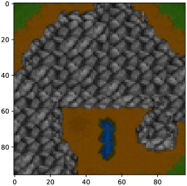
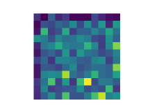
in lieu of . The observed data is called the context. As an illustrative running example, consider the shortest path prediction problem shown in Figure 1, which is studied in Berthet et al. (2020) and Pogančić et al. (2019).
At first glance, it may appear natural to tune the weights so as to minimize the difference between and . However, this is only possible if is available at training time. Even if this approach is feasible, it may not be advisable. If is a near-perfect predictor of we can expect . However, if there are even small differences between and this can manifest in wildly different solutions (Bengio, 1997; Wilder et al., 2019). Thus, we focus on methods where is tuned by minimizing the discrepancy between and . Such methods are instances of the decision-focused learning paradigm Mandi et al. (2023), as the criterion we are optimizing for is the quality of (the “decision”) not the fidelity of (the “prediction”).
The key obstacle in using gradient-based algorithms to tune in such approaches is “differentiating through” the solution of equation 2 to obtain a gradient with which to update . Specifically, the combinatorial nature of may cause the solution to remain unchanged for many small perturbations to ; yet, for some perturbations may “jump” to a different point in . Hence, the gradient is always either zero or undefined. To compute an informative gradient, we follow Wilder et al. (2019) by relaxing equation 2 to a quadratic program over the convex hull of with an added regularizer (see equation 8).
 |
 |
 |
Contribution
Drawing upon recent advances in convex optimization (Ryu & Yin, 2022) and implicit neural networks (Fung et al., 2022; McKenzie et al., 2021), we propose a method designed specifically for “differentiating through” large-scale integer linear programs. Our approach is fast, easy to implement using our provided code, and, unlike several prior works (e.g. see Pogančić et al. (2019); Berthet et al. (2020)), trains completely on GPU. Numerical examples herein demonstrate our approach, run using only standard computing resources, easily scales to problems with tens of thousands of variables. Theoretically, we verify our approach computes an informative gradient via a refined analysis of Jacobian-free Backpropagation (JFB) (Fung et al., 2022). In summary, we do the following.
-
We provide theoretical guarantees for differentiating through the fixed point of a certain non-expansive, but not contractive, operator.
-
We numerically show DYS-Net easily handles combinatorial problems with tens of thousands of variables.
2 Preliminaries
LP Reformulation
We focus on optimization problems of the form equation 1 where and is the integer or binary points of a polytope, which we may assume to be expressed in standard form (Ziegler, 2012):
| (3) |
In other words, equation 1 is an Integer Linear Program (ILP). Similar to works by Elmachtoub & Grigas (2022); Wilder et al. (2019); Mandi & Guns (2020) and others we replace the model equation 2 with its continuous relaxation, and redefine
| (4) |
as a step towards making the computation of feasible.
Losses and Training Data
We assume access to training data in the tuple form . Such data may be obtained by observing experienced agents solve equation 1, for example taxi drivers in a shortest path problem Piorkowski et al. (2009). We focus on the loss:
| (5) |
and is the distribution of contextual data, although more sophisticated losses can be used with only superficial changes to our results. In principle we select the optimal weights by solving . In practice, the population risk is inaccessible, and so we minimize empirical risk instead (Vapnik, 1999):
| (6) |
Argmin Differentiation
For notational brevity, we temporarily suppress the dependence on . The gradient of with respect to , evaluated on a single data point is
As discussed in Section 1, is piecewise constant as a function of , and this remains true for the LP relaxation equation 4. Consequently, for all , either or is undefined—neither case yields an informative gradient. To remedy this, Wilder et al. (2019); Mandi & Guns (2020) propose adding a small amount of regularization to the objective function in equation 4 to make it strongly convex. This ensures is a continuously differentiable function of . We add a small quadratic regularizer, modulated by , to obtain the objective
| (7) |
and henceforth replace equation 4 by
| (8) |
During training, we aim to solve equation 8 and efficiently compute the derivative .
Pitfalls of Relaxation
Finally, we offer a note of caution when using the quadratically regularized problem equation 8 as a proxy for the original integer linear program equation 1. Temporarily defining
we observe that two sources of error have arisen; one from replacing with (i.e. the discrepancy between and ), and one from replacing the linear objective function with its quadratically regularized counterpart (i.e. the discrepancy between and ). When is totally unimodular, is guaranteed to be integral, in which case . Moreover, Wilder et al. (2019, Theorem 2) shows that
whence, as in the proof Berthet et al. (2020, Proposition 2.2), (at least when is compact). Thus, for totally unimodular ILPs (e.g. the shortest path problem), it is reasonable to expect that obtained from equation 8, for well-tuned and small , are of acceptable quality. For ILPs which are not totally unimodular no such theoretical guarantees exist. However, we observe that this relaxation works reasonably well, at least for the knapsack problem.
3 Related Works
We highlight recent works in decision-focused learning—particularly for mixed integer programs—and related areas.
Optimization Layers
Introduced in Amos & Kolter (2017), and studied further in Agrawal et al. (2019b; c); Bolte et al. (2021); Blondel et al. (2022), an optimization layer is a modular component of a deep learning framework where forward propagation consists of solving a parametrized optimization problem. Consequently, backpropagation entails differentiating the solution to this problem with respect to the parameters. Optimization layers are a promising technology as they are able to incorporate hard constraints into deep neural networks. Moreover, as their output is a (constrained) minimizer of the objective function, it is easier to interpret than the output of a generic layer.
Decision-focused learning for LPs
When an optimization layer is fitted to a data-dependent optimization problems of the form equation 1, with the goal of maximizing the quality of the predicted solution, this is usually referred to as decision-focused learning. We narrow our focus to the case where the objective function in equation 1 is linear.Wilder et al. (2019) and Elmachtoub & Grigas (2022) are two of the earliest works applying deep learning techniques to data-driven LPs, and delineate two fundamentally different approaches. Specifically, Wilder et al. (2019) proposes replacing the LP with a continuous and strongly convex relaxation, as described in Section 2. This approach is extended to ILPs in Ferber et al. (2020), and to non-quadratic regularizers in Mandi & Guns (2020). On the other hand, Elmachtoub & Grigas (2022) avoid modifying the underlying optimization problem and instead propose a new loss function; dubbed the Smart Predict-then-Optimize (SPO) loss, to be used instead of the loss. We emphasize that the SPO loss requires access to the true cost vectors , a setting which we do not consider.
Several works define a continuously differentiable proxy for the solution to the unregularized LP equation 4, which we rewrite here as111For sake of notational simplicity, the dependence on is implicit.
| (9) |
In Berthet et al. (2020), a stochastic perturbation is considered:
| (10) |
which is somewhat analogous to Nesterov-Spokoiny smoothing (Nesterov & Spokoiny, 2017) in zeroth-order optimization. For some draws of the additively perturbed cost vector may have negative entries, which may cause a solver (e.g. Dijkstra’s algorithm) applied to the associated LP to fail. To avoid this, Dalle et al. (2022) suggest using a multiplicative perturbation of instead.
Pogančić et al. (2019) define a piecewise-affine interpolant to , where is a suitable loss function.
We note a bifurcation in the literature; Wilder et al. (2019); Ferber et al. (2020); Elmachtoub & Grigas (2022) assume access to training data of the form , whereas Pogančić et al. (2019); Berthet et al. (2020); Sahoo et al. (2022) use training data of the form . The former setting is frequently referred to as the predict-then-optimize problem. Our focus is on the latter setting. We refer the reader to Kotary et al. (2021); Mandi et al. (2023) for recent surveys of this area.
Deep Equilibrium Models
Bai et al. (2019); El Ghaoui et al. (2021) propose the notion of deep equilibrium model (DEQ), also known as an implicit neural network. A DEQ is a neural network for which forward propagation consists of (approximately) computing a fixed point of a parametrized operator. We note that equation 8 may be reformulated as a fixed point problem,
| (11) |
where is the orthogonal projection222For a set , . onto . Thus, DEQ techniques may be applied to constrained optimization layers (Chen et al., 2021; Blondel et al., 2022; McKenzie et al., 2021). However, the cost of computing can be prohibitive, see the discussion in Section 4.
Learning-to-Optimize (L2O)
Our work is related to the learning-to-optimize (L2O) framework (Chen et al., 2022; Li & Malik, 2017; Chen et al., 2018; Liu et al., 2023), where an optimization algorithm is learned and its outputs are used to perform inferences. However, traditional L2O methods use a fixed number of layers (i.e. unrolled algorithms). Our approach attempts to differentiate through the solution and is therefore most closely aligned with works that employ implicit networks within the L2O framework (Amos & Kolter, 2017; Heaton & Fung, 2023; McKenzie et al., 2021; Gilton et al., 2021; Liu et al., 2022). We highlight that, unlike many L2O works, our goal is not to learn a faster optimization method for fully specified problems. Rather, we seek to solve partially specified problems given contextual data by combining learning and optimization techniques.
Computing the derivative of a minimizer with respect to parameters
In all of the aforementioned works, the same fundamental problem is encountered: must be computed where is the solution of a (constrained) optimization problem with objective function parametrized by . The most common approach to doing so, proposed in Amos & Kolter (2017) and used in Ruthotto et al. (2018); Wilder et al. (2019); Mandi & Guns (2020); Ferber et al. (2020), starts with the KKT conditions for constrained optimality:
where and are Lagrange multipliers associated to the optimal solution (Bertsekas, 1997) and is a matrix with along its diagonal. Differentiating these equations with respect to and rearranging yields
| (12) |
The matrix and right hand side vector in equation 12 are computable, thus enabling one to solve for (as well as and ). We emphasize that both primal (i.e., ) and dual (i.e., and ) variables at optimality are required. This constrains the choice of optimization schemes to those that track primal and dual variables, and prohibits the use of fast, primal-only schemes. Following (Amos & Kolter, 2017), most works employing this approach use a primal-dual interior point method, which computes acceptable approximations to , , and at a cost of , assuming
and .
Using the stochastic proxy equation 10, Berthet et al. (2020) derive a formula for which is also an expectation, and hence can be efficiently approximated using Monte Carlo methods. Pogančić et al. (2019) show that the gradients of their interpolant are strikingly easy to compute, requiring just one additional solve of equation 9 with perturbed cost . This approach is extended by Sahoo et al. (2022) which proposes to avoid computing entirely, replacing it with the negative identity matrix. This is similar in spirit to our use of Jacobian-free Backpropagation (see Section 4).
4 DYS-Net
We now introduce our proposed model, DYS-net. We use this term to refer to the model and the training procedure. Fixing an architecture for , and an input , DYS-net computes an approximation to in a way that is easy to backpropagate through:
| (13) |
The Forward Pass
As we wish to compute and for high dimensional settings (i.e. large ), we eschew second-order methods (e.g. Newton’s method) in favor of first-order methods such as projected gradient descent (PGD). With PGD, a sequence of estimates of are computed so that where
This approach works for simple sets for which there exists an explicit form of , e.g. when is the probability simplex (Duchi et al., 2008; Condat, 2016; Li et al., 2023). However, for general polytopes no such form exists, thereby requiring a second iterative procedure to compute . This projection must be computed at every iteration of every forward pass for every sample of every epoch, and this dominates the computational cost, see McKenzie et al. (2021, Appendix 4).
To avoid this expense, we draw on recent advances in the convex optimization literature, particularly Davis-Yin splitting or DYS (Davis & Yin, 2017). DYS is a three operator splitting technique, and hence is able to decouple the polytope constraints into relatively simple constraints Davis & Yin (2017). This technique has been used elsewhere, e.g. Pedregosa & Gidel (2018); Yurtsever et al. (2021). Specifically, we adapt the architecture incorporating DYS proposed in McKenzie et al. (2021). To this end, we rewrite as
| (14) |
While is hard to compute, both and can be computed cheaply via explicit formulas, once a singular value decomposition (SVD) is computed for . We verify this via the following lemma (included for completeness, as the two results are already known).
Lemma 1.
If are as in equation 14 and is full-rank then:
-
1.
, where and is the compact SVD of .
-
2.
.
We remark that the SVD of is computed offline, and is a once-off cost. Alternatively, one could compute by using an iterative method (e.g. GMRES) to find the (least squares) solution to , whence , but this would need to be done at each iteration of each forward pass for every sample of every epoch. Thus, it is unclear whether this procides computational savings over the once-off computation of the SVD. However, this could prove useful when is only provided implicitly, i.e. via access to a matrix-vector product oracle.
The following theorem allows one to approximate using only and , not .
Theorem 2.
A full proof is included in Appendix A; here we provide a proof sketch. Substituting the gradient
for into the formula for given in McKenzie et al. (2021, Theorem 3.2) and rearranging yields equation 16. Verifying the assumptions of McKenzie et al. (2021, Theorem 3.3) are satisfied is straightforward. For example, is -cocoercive by the Baillon-Haddad theorem (Baillon & Haddad, 1977; Bauschke & Combettes, 2009).
The forward pass of DYS-net consists of iterating equation 15 until a suitable stopping criterion is met. For simplicity, in presenting Algorithm 1 we assume this to be a maximum number of iterations is reached. One may also consider a stopping criterion of .
The Backward Pass
From Theorem 2, we deduce the following fixed point condition:
| (17) |
As discussed in McKenzie et al. (2021), instead of backpropagating through every iterate of the forward pass, we may derive a formula for by appealing to the implicit function theorem and differentiating both sides of equation 17:
| (18) |
We notice two immediate problems not addressed by McKenzie et al. (2021): (i) is not everywhere differentiable with respect to , as is not; (ii) if were a contraction (i.e. Lipschitz in with constant less than ), then would be invertible. However, this is not necessarily the case. Thus, it is not clear a priori that equation 18 can be solved for . Our key result (Theorem 6 below) is to provide reasonable conditions under which is invertible.
Assuming these issues can be resolved, one may compute the gradient of the loss using the chain rule:
This approach requires solving a linear system with which becomes particularly expensive when is large. Instead, we use Jacobian-free Backpropagation (JFB) (Fung et al., 2022), also known as one-step differentiation (Bolte et al., 2024), in which the Jacobian is replaced with the identity matrix. This leads to an approximation of the true gradient using
| (19) |
This update can be seen as a zeroth order Neumann expansion of Fung et al. (2022); Bolte et al. (2024). We show equation 19 is a valid descent direction by resolving the two problems highlighted above. We begin by rigorously deriving a formula for . Recall the following generalization of the Jacobian to non-smooth operators due to Clarke (1983).
Definition 3.
For any locally Lipschitz let denote the set upon which is differentiable. The Clarke Jacobian of is the set-valued function defined as
Where denotes the convex hull of a set.
The Clarke Jacobian of is easily computable, see Lemma 9. Define the (set-valued) functions
Then
| (20) |
where is applied element-wise. We shall now provide a consistent rule for selecting, at any , an element of . If for all then is a singleton. If one or more then is multi-valued, so we choose the element of with in the position for every . We write for this chosen element, and note that
This aligns with the default rule for assigning a sub-gradient to used in the popular machine learning libraries TensorFlow(Abadi et al., 2016), PyTorch (Paszke et al., 2019) and JAX (Bradbury et al., 2018), and has been observed to yield networks which are more stable to train than other choices (Bertoin et al., 2021).
Given the above convention, we can compute , interpreted as an element of the Clarke Jacobian of chosen according to a consistent rule. Surprisingly, may be expressed using only orthogonal projections to hyperplanes. Throughout, we let be the one-hot vector with in the -th position and zeros elsewhere, and be the -th row of . For any subspace we denote the orthogonal subspace as . The following theorem, the proof of which is given in Appendix A, characterizes .
Theorem 4.
Suppose is full-rank and , . Then for all
| (21) |
To show JFB is applicable, it suffices to verify when evaluated at . Theorem 4 enables us to show this inequality holds when satisfies a commonly-used regularity condition, which we formalize as follows.
Definition 5 (LICQ condition, specialized to our case).
Let denote the solution to equation 8. Let denote the set of active positivity constraints:
| (22) |
The point satisfies the Linear Independence Constraint Qualification (LICQ) condition if the vectors
| (23) |
are linearly independent.
Theorem 6.
If the LICQ condition holds at , is full-rank and , then .
The significance of Theorem 6, which is proved in Appendix A, is outlined by the following corollary, stating that using instead of the true gradient is still guaranteed to decrease , at least for small enough step-size.
Corollary 7.
If is continuously differentiable with respect to at , the assumptions in Theorem 6 hold and has condition number sufficiently small, then is a descent direction for with respect to .
Synergy between forward and backward pass
We highlight that the pseudogradient computed in the backward pass (i.e., ) does not require any Lagrange multipliers, in contrast with the gradient computed using equation 12. This is why we may use Davis-Yin splitting, as opposed to a primal-dual interior point method, on the forward pass. This allows efficiency gains on the forward pass, as Davis-Yin splitting scales favorably with the problem dimension.
Implementation
DYS-net is implemented as an abstract PyTorch (Paszke et al., 2019) layer in the provided code. To instantiate it, a user only need specify and (see equation 3) and choose an architecture for . At test time, it can be beneficial to solve the underlying combinatorial problem equation 2 exactly using a specialized algorithm, e.g. commercial integer programming software for the knapsack prediction problem. This can easily be done using DYS-net by instantiating the test-time-forward abstract method.
5 Numerical Experiments
We demonstrate the effectiveness of DYS-Net through four experiments. In all our experiments with DYS-net we used and , with an early stopping condition of with . We compare DYS-net against three other methods: Perturbed Optimization (Berthet et al., 2020)—PertOpt-net; an approach using Blackbox Backpropagation (Vlastelica et al., 2019)—BB-net; and an approach using cvxpylayers (Agrawal et al., 2019a)—CVX-net. All code needed to reproduce our experiments is available at https://github.com/mines-opt-ml/fpo-dys.
5.1 Experiments using PyEPO
First, we verify the efficiency of DYS-net by performing benchmarking experiments within the PyEPO (Tang & Khalil, 2022) framework.
Models
We use the PyEPO implementations of Perturbed Optimization, respectively Blackbox Backpropagation, as the core of PertOpt-net, respectively BB-net. We use the same architecture for for all models333The architecture we use for shortest path prediction problems differs from that used for knapsack prediction problems. See the appendix for details. and use an appropriate combinatorial solver at test time, via the PyEPO interface to Gurobi. Thus, the methods differ only in training procedure. The precise architectures used for for each problem are described in Appendix C, and are also viewable in the accompanying code repository. Interestingly, we observed that adding drop-out during training to the output layer proved beneficial for the knapsack prediction problem. Without this, we find that tends to output a sparse approximation to supported on a feasible set of items, and so does not generalize well.
Training
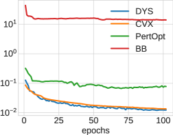
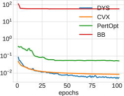
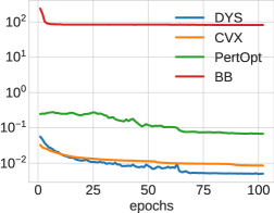
We train for a maximum of 100 epochs or 30 minutes, whichever comes first. We use a validation set for model selection as we observe that, for all methods, the best loss is seldom achieved at the final iteration. Exact hyperparameters are discussed in Appendix C. For each problem size, we perform three repeats with different randomly generated data. Results are displayed in Figure 2.
Evaluation
Given test data and a fully trained model we define the regret:
| (24) |
Note that regret is non-negative, and is zero precisely when is a solution of equal quality to . Following Tang & Khalil (2022), we evaluate the quality of using normalized regret, defined as
| (25) |
5.1.1 Shortest Path Prediction
The shortest path between two vertices in a graph can be found by:
| (26) |
where is the vertex-edge adjacency matrix, encodes the initial and terminal vertices, and is a vector encoding (-dependent) edge lengths. Here, will encode the edges included in the optimal path. In this experiment we focus on the case where is the grid graph. We use the PyEPO Tang & Khalil (2022) benchmarking software to generate training datasets of the form where for each . The are sampled from the five-dimensional multivariate Gaussian distribution with mean and identity covariance. Note that the number of variables in equation 26 scales like , not .
5.1.2 Knapsack Prediction
In the (0–1, single) knapsack prediction problem, we are presented with a container (i.e. a knapsack) of size and items, of sizes and values . The goal is to select the subset of maximum value that fits in the container, i.e. to solve:
Here, encodes the selected items. In the (0–1) -knapsack prediction problem we imagine the container having various notions of “size” (i.e. length, volume, weight limit) and hence a -tuple of capacities . Correspondingly, the items each have a -tuple of sizes . We aim to select a subset of maximum value, amongst all subsets satisfying the capacity constraints:
| (27) |
In Appendix B we discuss how to transform into the canonical form discussed in Section 2. We again use PyEPO to generate datasets of the form where for and varying from to inclusive in increments of . The from the five-dimensional multivariate Gaussian distribution with mean and identity covariance.
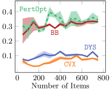
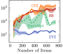
5.1.3 Results
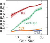
As is clear from Figure 2 DYS-net trains the fastest among the four methods, and achieves the best or near-best normalized regret in all cases. We attribute the accuracy to the fact that it is not a zeroth order method. Moreover, avoiding computation and backpropagation through the projection allows DYS to have fast runtimes.
5.2 Large-scale shortest path prediction
Our shortest path prediction experiment described in Section 5.1.1 is bottlenecked by the fact that the “academic” license of Gurobi does not allow for shortest path prediction problems on grids larger than . To further explore the limits of DYS-net, we redo this experiment using a custom pyTorch implementation of Dijkstra’s algorithm444adapted from Tensorflow code available at https://github.com/google-research/google-research/blob/master/perturbations/experiments/shortest_path.py as our base solver for equation 26.
Data Generation
We generate datasets for -by- grids where and the are sampled uniformly at random from , the true edge weights are computed as for fixed , and is computed given using the aforementioned pyTorch implementation of Dijkstra’s algorithm. Thus, all entries of are non-negative, and are positive with overwhelming probability.
| grid size | number of variables | neural network size |
|---|---|---|
| 5-by-5 | 40 | 500 |
| 10-by-10 | 180 | 2040 |
| 20-by-20 | 760 | 8420 |
| 30-by-30 | 1740 | 19200 |
| 50-by-50 | 4900 | 53960 |
| 100-by-100 | 19800 | 217860 |
Models and Training
We test the same four approaches as in Sections 5.1.1 and 5.1.2, but unlike in these sections we do not use the PyEPO implementations of PertOpt-net or BB-net. We cannot, as the PyEPO implementations call Gurobi to solve equation 26 which, as mentioned above, cannot handle grids larger than . Instead, we use custom implementations based on the code accompanying the works introducing PertOpt (Berthet et al., 2020) and BB (Vlastelica et al., 2019). We use the same architecture for for DYS-net, PertOpt-net, and Cvx-net; a two layer fully connected neural network with leaky ReLU activation functions. For DYS-net and Cvx-net we do not modify the forward pass at test time. For BB-net we use a larger network by making the latent dimension 20-times larger than that of the first three as we found this more effective. Network sizes can be seen in Table 1.
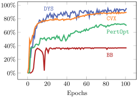
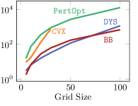
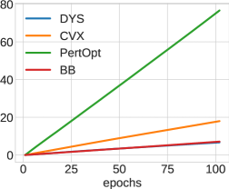
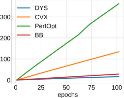
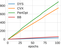
We tuned the hyperparameters for each approach to the best of our ability on the smallest problem (5-by-5 grid) and then used these hyperparameter values for all other graph sizes. See Figure 3 for the results of this training run. We train all approaches for 100 epochs total on each problem using the loss equation 5.
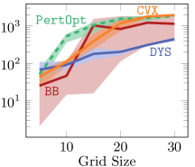
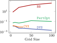
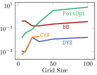
Results
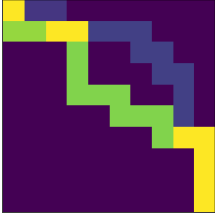
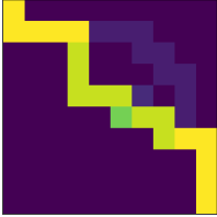
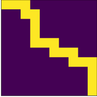
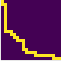
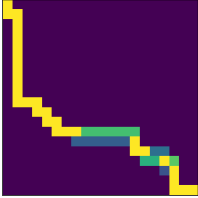
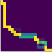
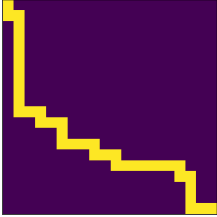
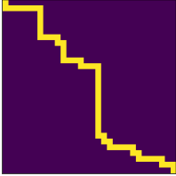
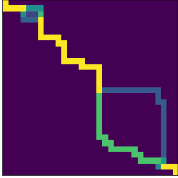
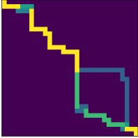
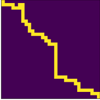
The results are displayed in Figure 4. While CVX-net and PertOpt-net achieve low regret for small grids, DYS-net model achieves a low regret for all grids. In addition to training faster, DYS-net can also be trained for much larger problems, e.g., 100-by-100 grids, as shown in Figure 4. We found that CVX-net could not handle grids larger than 30-by-30, i.e. , problems with more than 1740 variables555This is to be expected, as discussed in in Amos & Kolter (2017); Agrawal et al. (2019a) (see Table 1). Importantly, PertOpt-net takes close to a week to train for the 100-by-100 problem, whereas DYS-net takes about a day (see right Figure 4b). On the other hand, the training speed of BB-net is comparable to that of DYS-net, but does not lead to competitive accuracy as shown in Figure 4(a). Interpreting the outputs of DYS-net and CVX-net as (unnormalized) probabilities over the grid, one can use a greedy algorithm to determine the most probable path from top-left to bottom-right. For small grids, e.g. 5-by-5, this path coincides exactly with the true path for most (see Fig. 3).
5.3 Warcraft shortest path prediction
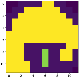
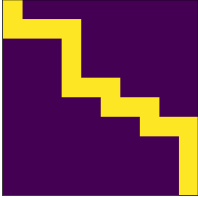
Finally, as an illustrative example, we consider the Warcraft terrains dataset first studied in Vlastelica et al. (2019). As shown in Figure 1, is a 96-by-96 RGB image, divided into a 12-by-12 grid of terrain tiles. Each tile has a different cost to traverse, and the goal is to find the quickest path from the top-left corner to the bottom-right corner.
Models, Training, and Evaluation
We build upon the code provided as part of the PyEPO package (Tang & Khalil, 2022). We use the same architecture for for BB-net, PertOpt-net, and DYS-net—a truncated ResNet18 (He et al., 2016) as first proposed in Vlastelica et al. (2019). We train each network for 50 epochs, except for the baseline. The initial learning rate is and it is decreased by a factor of 10 after 30 and 40 epochs respectively. PertOpt-net and DYS-net are trained to minimize the loss equation 5, while BB-net is trained to minimize the Hamming loss as described in Vlastelica et al. (2019). We evaluate the quality of using normalized regret equation 25.
Results
The results for this experiment are shown in Table 2. Interestingly, BB-net and PertOpt-net are much more competitive in this experiment than in the experiments of Sections 5.1.1, 5.1.2, and 5.2. We attribute this to the “discrete” nature of the true cost vector —for the Warcraft problem entries of can only take on four, well-separated values—as opposed to the more “continuous” nature of in the previous experiments. Thus, an algorithm that learns a rough approximation to the true cost vector will be more successful in the Warcraft problem than in the shortest path problems of Sections 5.1.1 and 5.2. This difference is illustrated in Figure 5. We also note that model selection using a validation set is beneficial for all approaches, but particularly so for BB-net and DYS-net, which achieve their best-performing models in the first several epochs of training.


| Algorithm | Test Normalized Regret | Time (in hours) |
|---|---|---|
| BB-net | ||
| PertOpt-net | ||
| DYS-net | ||
| CVX-net |
6 Conclusions
This work presents a new method for learning to solve ILPs using Davis-Yin splitting which we call DYS-net. We prove that the gradient approximation computed in the backward pass of DYS-net is indeed a descent direction, thus advancing the current understanding of implicit networks. Our experiments show that DYS-net is capable of scaling to truly large ILPs, and outperforms existing state-of-the-art methods, at least when training data is of the form . We note that in principle DYS-net may be applied given training data of the form ; a common paradigm for many predict-then-optimize problems Mandi et al. (2023). However, preliminary experiments showed that SPO+ Elmachtoub & Grigas (2022) achieved a substantially lower regret than DYS-net in this setting. We leave the extension of DYS-net to this data type to future work. Our experiments also reveal an interesting dichotomy between problems in which entries of may take on only a handful of discrete values and problems in which is more “continuous”. Future work could explore this dichotomy further, as well as apply DYS-net to additional ILPs, for example the traveling salesman problem.
References
- Abadi et al. (2016) Martin Abadi, Paul Barham, Jianmin Chen, Zhifeng Chen, Andy Davis, Jeffrey Dean, Matthieu Devin, Sanjay Ghemawat, Geoffrey Irving, Michael Isard, et al. Tensorflow: a system for large-scale machine learning. In 12th USENIX symposium on operating systems design and implementation (OSDI 16), pp. 265–283, 2016.
- Agrawal et al. (2019a) A. Agrawal, B. Amos, S. Barratt, S. Boyd, S. Diamond, and Z. Kolter. Differentiable convex optimization layers. In Advances in Neural Information Processing Systems, 2019a.
- Agrawal et al. (2019b) Akshay Agrawal, Brandon Amos, Shane Barratt, Stephen Boyd, Steven Diamond, and J Zico Kolter. Differentiable convex optimization layers. Advances in neural information processing systems, 32, 2019b.
- Agrawal et al. (2019c) Akshay Agrawal, Shane Barratt, Stephen Boyd, Enzo Busseti, and Walaa M Moursi. Differentiating through a cone program. arXiv preprint arXiv:1904.09043, 2019c.
- Amos & Kolter (2017) Brandon Amos and J Zico Kolter. Optnet: Differentiable optimization as a layer in neural networks. In International Conference on Machine Learning, pp. 136–145. PMLR, 2017.
- Bai et al. (2019) Shaojie Bai, J Zico Kolter, and Vladlen Koltun. Deep equilibrium models. Advances in Neural Information Processing Systems, 32, 2019.
- Baillon & Haddad (1977) Jean-Bernard Baillon and Georges Haddad. Quelques propriétés des opérateurs angle-bornés et n-cycliquement monotones. Israel Journal of Mathematics, 26:137–150, 1977.
- Bauschke & Combettes (2009) Heinz H Bauschke and Patrick L Combettes. The Baillon-Haddad theorem revisited. arXiv preprint arXiv:0906.0807, 2009.
- Bengio (1997) Yoshua Bengio. Using a financial training criterion rather than a prediction criterion. International journal of neural systems, 8(04):433–443, 1997.
- Berthet et al. (2020) Quentin Berthet, Mathieu Blondel, Olivier Teboul, Marco Cuturi, Jean-Philippe Vert, and Francis Bach. Learning with differentiable perturbed optimizers. Advances in neural information processing systems, 33:9508–9519, 2020.
- Bertoin et al. (2021) David Bertoin, Jérôme Bolte, Sébastien Gerchinovitz, and Edouard Pauwels. Numerical influence of ReLU’(0) on backpropagation. Advances in Neural Information Processing Systems, 34:468–479, 2021.
- Bertsekas (1997) Dimitri P Bertsekas. Nonlinear programming. Journal of the Operational Research Society, 48(3):334–334, 1997.
- Blondel et al. (2022) Mathieu Blondel, Quentin Berthet, Marco Cuturi, Roy Frostig, Stephan Hoyer, Felipe Llinares-López, Fabian Pedregosa, and Jean-Philippe Vert. Efficient and modular implicit differentiation. Advances in neural information processing systems, 35:5230–5242, 2022.
- Bolte et al. (2021) Jérôme Bolte, Tam Le, Edouard Pauwels, and Tony Silveti-Falls. Nonsmooth implicit differentiation for machine-learning and optimization. Advances in neural information processing systems, 34:13537–13549, 2021.
- Bolte et al. (2024) Jérôme Bolte, Edouard Pauwels, and Samuel Vaiter. One-step differentiation of iterative algorithms. Advances in Neural Information Processing Systems, 36, 2024.
- Bradbury et al. (2018) James Bradbury, Roy Frostig, Peter Hawkins, Matthew James Johnson, Chris Leary, Dougal Maclaurin, George Necula, Adam Paszke, Jake VanderPlas, Skye Wanderman-Milne, et al. Jax: composable transformations of python+ numpy programs. 2018.
- Chen et al. (2021) Bingqing Chen, Priya L Donti, Kyri Baker, J Zico Kolter, and Mario Bergés. Enforcing policy feasibility constraints through differentiable projection for energy optimization. In Proceedings of the Twelfth ACM International Conference on Future Energy Systems, pp. 199–210, 2021.
- Chen et al. (2022) Tianlong Chen, Xiaohan Chen, Wuyang Chen, Howard Heaton, Jialin Liu, Zhangyang Wang, and Wotao Yin. Learning to optimize: A primer and a benchmark. Journal of Machine Learning Research, 23(189):1–59, 2022.
- Chen et al. (2018) Xiaohan Chen, Jialin Liu, Zhangyang Wang, and Wotao Yin. Theoretical linear convergence of unfolded ista and its practical weights and thresholds. Advances in Neural Information Processing Systems, 31, 2018.
- Clarke (1983) FH Clarke. Optimization and nonsmooth analysis, wiley-interscience. New York, 1983.
- Condat (2016) Laurent Condat. Fast projection onto the simplex and the ball. Mathematical Programming, 158(1):575–585, 2016.
- Dalle et al. (2022) Guillaume Dalle, Léo Baty, Louis Bouvier, and Axel Parmentier. Learning with combinatorial optimization layers: a probabilistic approach. arXiv preprint arXiv:2207.13513, 2022.
- Davis & Yin (2017) Damek Davis and Wotao Yin. A three-operator splitting scheme and its optimization applications. Set-valued and variational analysis, 25(4):829–858, 2017.
- Duchi et al. (2008) John Duchi, Shai Shalev-Shwartz, Yoram Singer, and Tushar Chandra. Efficient projections onto the -ball for learning in high dimensions. In Proceedings of the 25th international conference on Machine learning, pp. 272–279, 2008.
- El Ghaoui et al. (2021) Laurent El Ghaoui, Fangda Gu, Bertrand Travacca, Armin Askari, and Alicia Tsai. Implicit deep learning. SIAM Journal on Mathematics of Data Science, 3(3):930–958, 2021.
- Elmachtoub & Grigas (2022) Adam N Elmachtoub and Paul Grigas. Smart “predict, then optimize”. Management Science, 68(1):9–26, 2022.
- Ferber et al. (2020) Aaron Ferber, Bryan Wilder, Bistra Dilkina, and Milind Tambe. Mipaal: Mixed integer program as a layer. In Proceedings of the AAAI Conference on Artificial Intelligence, volume 34, pp. 1504–1511, 2020.
- Fung et al. (2022) Samy Wu Fung, Howard Heaton, Qiuwei Li, Daniel McKenzie, Stanley Osher, and Wotao Yin. JFB: Jacobian-free backpropagation for implicit networks. In Proceedings of the AAAI Conference on Artificial Intelligence, 2022.
- Geng et al. (2021) Zhengyang Geng, Xin-Yu Zhang, Shaojie Bai, Yisen Wang, and Zhouchen Lin. On training implicit models. Advances in Neural Information Processing Systems, 34:24247–24260, 2021.
- Gilton et al. (2021) Davis Gilton, Gregory Ongie, and Rebecca Willett. Deep equilibrium architectures for inverse problems in imaging. IEEE Transactions on Computational Imaging, 7:1123–1133, 2021.
- (31) Jean Guyomarch. Warcraft ii open-source map editor, 2017. http://github. com/war2/war2edit.
- He et al. (2016) Kaiming He, Xiangyu Zhang, Shaoqing Ren, and Jian Sun. Deep residual learning for image recognition. In Proceedings of the IEEE conference on computer vision and pattern recognition, pp. 770–778, 2016.
- Heaton & Fung (2023) Howard Heaton and Samy Wu Fung. Explainable ai via learning to optimize. Scientific Reports, 13(1):10103, 2023.
- Kacem et al. (2021) Imed Kacem, Hans Kellerer, and A Ridha Mahjoub. Preface: New trends on combinatorial optimization for network and logistical applications. Annals of Operations Research, 298(1):1–5, 2021.
- Karp (1972) Richard M Karp. Reducibility among combinatorial problems. In Complexity of computer computations, pp. 85–103. Springer, 1972.
- Kotary et al. (2021) James Kotary, Ferdinando Fioretto, Pascal van Hentenryck, and Bryan Wilder. End-to-end constrained optimization learning: A survey. In 30th International Joint Conference on Artificial Intelligence, IJCAI 2021, pp. 4475–4482. International Joint Conferences on Artificial Intelligence, 2021.
- Li & Malik (2017) Ke Li and Jitendra Malik. Learning to optimize. In International Conference on Learning Representations, 2017.
- Li et al. (2023) Qiuwei Li, Daniel McKenzie, and Wotao Yin. From the simplex to the sphere: faster constrained optimization using the hadamard parametrization. Information and Inference: A Journal of the IMA, 12(3):1898–1937, 2023.
- Liao et al. (2018) Renjie Liao, Yuwen Xiong, Ethan Fetaya, Lisa Zhang, KiJung Yoon, Xaq Pitkow, Raquel Urtasun, and Richard Zemel. Reviving and improving recurrent back-propagation. In International Conference on Machine Learning, pp. 3082–3091. PMLR, 2018.
- Liu et al. (2023) Jialin Liu, Xiaohan Chen, Zhangyang Wang, Wotao Yin, and HanQin Cai. Towards constituting mathematical structures for learning to optimize. In International Conference on Machine Learning, pp. 21426–21449. PMLR, 2023.
- Liu et al. (2022) Jiaming Liu, Xiaojian Xu, Weijie Gan, Ulugbek Kamilov, et al. Online deep equilibrium learning for regularization by denoising. Advances in Neural Information Processing Systems, 35:25363–25376, 2022.
- Mandi & Guns (2020) Jayanta Mandi and Tias Guns. Interior point solving for lp-based prediction+ optimisation. Advances in Neural Information Processing Systems, 33:7272–7282, 2020.
- Mandi et al. (2023) Jayanta Mandi, James Kotary, Senne Berden, Maxime Mulamba, Victor Bucarey, Tias Guns, and Ferdinando Fioretto. Decision-focused learning: Foundations, state of the art, benchmark and future opportunities. arXiv preprint arXiv:2307.13565, 2023.
- McKenzie et al. (2021) Daniel McKenzie, Howard Heaton, Qiuwei Li, Samy Wu Fung, Stanley Osher, and Wotao Yin. Operator splitting for learning to predict equilibria in convex games. arXiv e-prints, pp. arXiv–2106, 2021.
- Nesterov & Spokoiny (2017) Yurii Nesterov and Vladimir Spokoiny. Random gradient-free minimization of convex functions. Foundations of Computational Mathematics, 17:527–566, 2017.
- Paszke et al. (2019) Adam Paszke, Sam Gross, Francisco Massa, Adam Lerer, James Bradbury, Gregory Chanan, Trevor Killeen, Zeming Lin, Natalia Gimelshein, Luca Antiga, et al. Pytorch: An imperative style, high-performance deep learning library. Advances in Neural Information Processing Systems, 32, 2019.
- Pedregosa & Gidel (2018) Fabian Pedregosa and Gauthier Gidel. Adaptive three operator splitting. In International Conference on Machine Learning, pp. 4085–4094. PMLR, 2018.
- Piorkowski et al. (2009) Michal Piorkowski, Natasa Sarafijanovic-Djukic, and Matthias Grossglauser. Crawdad data set epfl/mobility (v. 2009-02-24), 2009.
- Pogančić et al. (2019) Marin Vlastelica Pogančić, Anselm Paulus, Vit Musil, Georg Martius, and Michal Rolinek. Differentiation of blackbox combinatorial solvers. In International Conference on Learning Representations, 2019.
- Ruthotto et al. (2018) Lars Ruthotto, Julianne Chung, and Matthias Chung. Optimal experimental design for inverse problems with state constraints. SIAM Journal on Scientific Computing, 40(4):B1080–B1100, 2018.
- Ryu & Yin (2022) Ernest Ryu and Wotao Yin. Large-Scale Convex Optimization: Algorithm Designs via Monotone Operators. Cambridge University Press, Cambridge, England, 2022.
- Sahoo et al. (2022) Subham Sekhar Sahoo, Anselm Paulus, Marin Vlastelica, Vít Musil, Volodymyr Kuleshov, and Georg Martius. Backpropagation through combinatorial algorithms: Identity with projection works. In The Eleventh International Conference on Learning Representations, 2022.
- Sbihi & Eglese (2010) Abdelkader Sbihi and Richard W Eglese. Combinatorial optimization and green logistics. Annals of Operations Research, 175(1):159–175, 2010.
- Tang & Khalil (2022) Bo Tang and Elias Boutros Khalil. Pyepo: A pytorch-based end-to-end predict-then-optimize library with linear objective function. In OPT 2022: Optimization for Machine Learning (NeurIPS 2022 Workshop), 2022.
- Vapnik (1999) Vladimir Vapnik. The nature of statistical learning theory. Springer science & business media, 1999.
- Vlastelica et al. (2019) Marin Vlastelica, Anselm Paulus, Vit Musil, Georg Martius, and Michal Rolinek. Differentiation of blackbox combinatorial solvers. In International Conference on Learning Representations, 2019.
- Wang & Tang (2021) Qi Wang and Chunlei Tang. Deep reinforcement learning for transportation network combinatorial optimization: A survey. Knowledge-Based Systems, 233:107526, 2021.
- Wilder et al. (2019) Bryan Wilder, Bistra Dilkina, and Milind Tambe. Melding the data-decisions pipeline: Decision-focused learning for combinatorial optimization. In Proceedings of the AAAI Conference on Artificial Intelligence, volume 33, pp. 1658–1665, 2019.
- Yurtsever et al. (2021) Alp Yurtsever, Varun Mangalick, and Suvrit Sra. Three operator splitting with a nonconvex loss function. In International Conference on Machine Learning, pp. 12267–12277. PMLR, 2021.
- Zhong & Tang (2021) Liwei Zhong and Guochun Tang. Preface: Combinatorial optimization drives the future of health care. Journal of Combinatorial Optimization, 42(4):675–676, 2021.
- Ziegler (2012) Günter M Ziegler. Lectures on polytopes, volume 152. Springer Science & Business Media, 2012.
Appendix A Appendix A: Proofs
For the reader’s convenience we restate each result given in the main text before proving it.
Theorem 2. Let be as in equation 14, and suppose for any neural network . For any define the sequence by:
| (28) |
where
| (29) |
If then the sequence converges to in equation 8 and .
Proof.
First note that . Because is strongly convex, is unique and is characterized by the first order optimality condition:
| (30) |
Note that equation 30 can equally be viewed as a variational inequality with operator . We deduce that with is a fixed point of
| (31a) | ||||
| (31b) | ||||
from McKenzie et al. (2021, Theorem 4.2), which is itself a standard application of ideas from operator splitting (Davis & Yin, 2017; Ryu & Yin, 2022).
As is -Lipschitz continuous it is also is -cocoercive by the Baillon-Haddad theorem (Baillon & Haddad, 1977; Bauschke & Combettes, 2009). McKenzie et al. (2021, Theorem 3.3) then implies that and . However, this theorem does not give a convergence rate. In fact, the convergence rate can be deduced from known results; because is averaged for the rate follows from Ryu & Yin (2022, Theorem 1).
Thus,
| (32) |
as desired.
∎
Next, we state two auxiliary lemmas relating the Jacobian matrices to projections onto linear subspaces.
Lemma 8.
If , for full-rank , with , and then
| (33) |
Proof.
Let denote the reduced SVD of , and note that as with we have and . Differentiating the formula for given in Lemma 1 yields
| (34) |
where . Note
| (35) |
which is the orthogonal projection onto . It follows that is the orthogonal projection on to . ∎
Lemma 9.
Define the multi-valued function
| (36) |
and, for , define . Then
| (37) |
and adopting the convention for choosing an element of stated in the main text:
| (38) |
Proof.
First, suppose satisfies , for all , i.e. is a smooth point of . Note
| (39) |
Thus, the Jacobian matrix is diagonal with a in the -th position whenever and otherwise, i.e. . Now suppose for one . For all with , the Jacobian is well-defined and has a 0 in the -th position, while for with , the Jacobian is well-defined and has a 1 in the -th position. Taking the convex hull yields the interval in the -th position, as claimed. The case where for multiple is similar.
Consequently, the product of and any vector equals if and only if . This shows the linear operator is idempotent with fixed point set , i.e. it is the projection operator . ∎
Theorem 4. Suppose is full-rank and , . Then for all
| (40) |
Proof.
Differentiating the expression for in equation 16 with respect to yields
| (41a) | ||||
| (41b) | ||||
where, for notational brevity, we set in the first line and the second line follows from Lemmas 8 and 9. Repeatedly using the fact, for any subspace , , the derivative can be further rewritten:
| (42a) | ||||
| (42b) | ||||
| (42c) | ||||
| (42d) | ||||
| (42e) | ||||
completing the proof. ∎
We use the following lemma to prove Theorem 6.
Lemma 10.
If the LICQ condition holds at , then .
Proof.
We first rewrite and . The subspace is spanned by all non-positive coordinates of . By equation 17, , and so if and only if . It follows that
| (43) |
where we enumerate via . On the other hand, where denotes the -th row of .
Let be given. Since , there are scalars such that Similarly, since , there are scalars such that Hence
| (44) |
By the LICQ condition, is a linearly independent set of vectors; hence and, thus, . Since was arbitrarily chosen in , the result follows. ∎
Theorem 6. If the LICQ condition holds at , is full-rank and , then .
Proof.
By Lemma 10, the LICQ condition implies . This implies that either (i) the first principal angle between these two subspaces is nonzero, and so the cosine of this angle is less than unity, i.e.
| (45) |
or (ii) (at least) one of is the trivial vector space . In either case, let be given. By Theorem 4, in case (ii)
| (46) |
implying that
| (47) |
where the inequality follows as projection operators are firmly nonexpansive. In case (i), write , where and . Appealing to Theorem 4 again
| (48) |
Pythagoras’ theorem may be applied to deduce, together with the fact and are orthogonal,
| (49) |
Since , the angle condition (45) implies
| (50) |
where the third equality holds since orthogonal linear projections are symmetric and idempotent. Because projections are non-expansive and is linear,
| (51) |
Combining (49), (50) and (51) reveals
| (52a) | ||||
| (52b) | ||||
| (52c) | ||||
Corollary 7. If is continuously differentiable with respect to at , the assumptions in Theorem 6 hold and has condition number sufficiently small, then is a descent direction for with respect to .
Proof.
Remark 11.
Similar guarantees, albeit with less restrictive assumptions on , can be deduced from the results of the recent work (Bolte et al., 2024).
Appendix B Derivation for Canonical Form of Knapsack Prediction Problem
For completeness, we explain how to transform the -knapsack prediction problem into the canonical form equation 8, and how to derive the standardized representation of the constraint polytope . Recall that the -knapsack prediction problem, as originally stated, is
| (54) |
We introduce slack variables so that the inequality constraint becomes
We relax the binary constraint to . We add additional slack variables to account for the upper bound:
| (55) |
Putting this together, define
| (56) |
Finally, redefine and (where we’re using to switch the argmax to an argmin) and obtain:
| (57) |
Appendix C Experimental Details
C.1 Additional Data Details for PyEPO problems
We use PyEPO (Tang & Khalil, 2022), specifically the functions data.shortestpath.genData and data.knapsack.genData to generate the training data. Both functions sample with with probability and with probability and then construct the cost vector as
where and is sampled uniformly from the interval . Note that is, by construction, non-negative.
C.2 Additional Model Details for PyEPO problems
For PertOpt-net and BBOpt-net we use the default hyperparameter values provided by PyEPO, namely for BBOpt-net, number of samples equal 3, and Gumbel noise for PertOpt-net. See Pogančić et al. (2019) and Berthet et al. (2020) respectively for descriptions of these hyperparameters. We do so as these are selected via hyperparameter tuning Tang & Khalil (2022). As DYS-net and CVX-net solve a regularized form of the underlying LP equation 7, the regularization parameter needs to be set. After experimenting with different values, we select for DYS-net and for CVX-net.
C.3 Additional Training Details for Knapsack Problem
For all models we use an initial learning rate of and a scheduler that reduces the learning rate whenever the validation loss plateaus. We also used weight decay with a parameter of .
C.4 Additional Model Details for Large-Scale Shortest Path Problem
Our implementation of PertOpt-net used a PyTorch implementation666See code at github.com/tuero/perturbations-differential-pytorch of the original TensorFlow code777See code at github.com/google-research/google-research/tree/master/perturbations associated to the paper Berthet et al. (2020). We experimented with various hyperparameter settings for 5-by-5 grids and found setting the number of samples equal to 3, the temperature (i.e. ) to 1 and using Gumbel noise to work best, so we used these values for all other shortest path experiments. Our implementation of BB-net uses the blackbox-backprop package888See code at https://github.com/martius-lab/blackbox-backprop associated to the paper Pogančić et al. (2019). We found setting to work best for 5-by-5 grids, so we use this value for all other shortest path experiments. Again, we select for DYS-net and for CVX-net
C.5 Additional Training Details for Large-Scale Shortest Path Problem
We use the MSE loss to train DYS-net, PertOpt-net, and CVX-net. We tried using the MSE loss with BB-net but this did not work well, so we used the Hamming (also known as 0–1) loss, as done in Pogančić et al. (2019).
To train DYS-net and CVX-net, we use an initial learning rate of and use a scheduler that reduces the learning rate whenever the test loss plateaus—we found this to perform the best for these two models. For PertOpt-net we found that using a fixed learning rate of performed the best. For BB-net, we performed a logarithmic grid-search on the learning rate between to and found that performed best; we also attempted adaptive learning rate schemes such as reducing learning rates on plateau but did not obtain improved performance.
C.6 Additional Model Details for Warcraft Experiment
For PertOpt-net and BBOpt-net we again use the default hyperparameter values provided by PyEPO, namely for BBOpt-net, number of samples equal 3, and Gumbel noise for PertOpt-net. We set for both CVX-net and DYS-net.
C.7 Hardware
All networks were trained using a AMD Threadripper Pro 3955WX: 16 cores, 3.90 GHz, 64 MB cache, PCIe 4.0 CPU and an NVIDIA RTX A6000 GPU.
Appendix D Additional Experimental Results
In Figure 6, we show the test loss and training time per epoch for all three architectures: DYS-net, CVX-net, and PertOpt-net for 10-by-10, 20-by-20, and 30-by-30 grids. In terms of MSE loss, CVX-net and DYS-net lead to comparable performance. In the second row of Figure 6, we observe the benefits of combining the three-operator splitting with JFB (Fung et al., 2022); in particular, DYS-net trains much faster. Figure 7 shows some randomly selected outputs for the three architectures once fully trained.
| 10-by-10 | 20-by-20 | 30-by-30 |
| Test MSE Loss | ||
 |
 |
 |
| Training Time (in minutes) | ||
 |
 |
 |
| True Path | DYS-net | CVX-net | PertOpt-net |
| 10-by-10 | |||
 |
 |
 |
 |
| 20-by-20 | |||
 |
 |
 |
 |
| 30-by-30 | |||
 |
 |
 |
 |