Diffraction integral computation using sinc approximation

Max Cubillos afrl.rdl.orgbox@us.af.mil Edwin Jimenez jimenez@caltech.edu Directed Energy Directorate, Air Force Research Laboratory, 3550 Aberdeen Ave SE, Kirtland AFB, Albuquerque, New Mexico 87117, USA Department of Computing and Mathematical Sciences, California Institute of Technology, 1200 E California Blvd, MC 305-16, Pasadena, California 91125, USA

Abstract

We propose a method based on sinc series approximations for computing the Rayleigh-Sommerfeld and Fresnel diffraction integrals of optics. The diffraction integrals are given in terms of a convolution, and our proposed numerical approach is not only super-algebraically convergent, but it also satisfies an important property of the convolution—namely, the preservation of bandwidth. Furthermore, the accuracy of the proposed method depends only on how well the source field is approximated; it is independent of wavelength, propagation distance, and observation plane discretization. In contrast, methods based on the fast Fourier transform (FFT), such as the angular spectrum method (ASM) and its variants, approximate the optical fields in the source and observation planes using Fourier series. We will show that the ASM introduces artificial periodic boundary conditions and violates the preservation of bandwidth property, resulting in limited accuracy which decreases for longer propagation distances. The sinc-based approach avoids both of these problems. Numerical results are presented for Gaussian beam propagation and circular aperture diffraction to demonstrate the high-order accuracy of the sinc method for both short-range and long-range propagation. For comparison, we also present numerical results obtained with the angular spectrum method.

keywords:

Fresnel diffraction , Rayleigh-Sommerfeld diffraction , angular spectrum method , sinc method

^†^†journal: Applied Numerical Mathematics

1 Introduction

One of the most basic problems in optics is the propagation of a known scalar optical field from one plane to another. Solutions to this problem are given in terms of various integrals—such as the Kirchoff, Rayleigh-Sommerfeld, Fresnel, and Fraunhofer integrals—with differing regimes of validity. These integrals have only a few analytical solutions, and therefore most optical propagation problems rely on numerical methods.

A variety of methods have been developed to evaluate the integrals of optics but the most popular are based on the convolution theorem and the FFT. In this article, we will compare our proposed approach to the standard FFT-based method: the angular spectrum method (ASM) [1, 2, 3, 4]. The ASM is also known by other names in the literature (such as the transfer function propagator [5]) and the name “angular spectrum method” is sometimes also used to refer to different methods. In optical propagation the unknown field at some observation plane is written in terms of a convolution of a diffraction kernel and a source field, and the ASM simply performs this computation as the inverse discrete Fourier transform of the product of the known Fourier transform of the kernel and the numerically computed Fourier transform of the source field [5, 4].

The fundamental problem with the ASM—as with other FFT-based methods—is that it approximates the optical field by a Fourier series, which introduces artificial periodicity into the domain. This artificial periodicity leads to errors from modes in the solution that should be scattered to infinity but are instead periodically reintroduced into the computational domain. The most straightforward way to reduce the errors caused by artificial periodicity is to increase the size of the domain, but at the cost of additional computation. There have been attempts to repair FFT-based methods, such as the band-limited angular spectrum method [6]; see also the recent article [7] and the references therein. Unfortunately, all such modifications only mitigate the artefacts of artificial periodicity under certain circumstances; they cannot eliminate the underlying problem entirely.

The problems that arise from using a Fourier basis for an infinite domain are naturally remedied by using a suitable set of basis functions such as the Whittaker cardinal basis or sinc functions, which are analytic in the whole complex plane. Methods based on sinc functions have a long history, dating back more than 100 years to the work of Borel [8] and Whittaker [9]. Since then, sinc methods have been used in a wide range of applications, including approximation theory, image processing, and the numerical solution of integral and differential equations; see the book [10] and references therein for a review of sinc-based methods. Although they have been used in a variety of computational physics problems, to our knowledge, sinc methods have not been applied to the problem of optical propagation.

In this article, we propose a new method for computing diffraction integrals based on approximation by sinc functions. For optical fields that are approximately bandlimited and decay exponentially in the transverse spatial direction, approximation by sinc functions is super-algebraically convergent [10, Chapter 1]. Furthermore, the only source of error is the approximation of the optical field; the error for computing the diffraction integral does not depend on wavelength, propagation distance, or observation plane grid. Although the method allows for arbitrary sample spacing in the source and observation planes, when the sampling is the same in both planes (a requirement of ASM), the FFT can be used to accelerate the computation. Thus, in this case, our sinc method has the same computational complexity as the ASM. However, in the near field, for an $N$ -point source grid, our sinc-based algorithm can be reduced to $\mathcal{O}(N)$ complexity, making it faster than any FFT-based method.

This article is organized as follows: Section 2 reviews the diffraction integrals covered in this article, emphasizing some of the important properties and their relevance to numerical methods. Section 3 discusses the ASM in the context of the arguments made in the preceding section together with related partial differential equations, showing why it is an inadequate method. Section 4 describes in detail the sinc-based method proposed in this article and shows how it naturally prevails where the ASM falls short. Finally, Section 5 presents numerical results showing, in practice, the advantages of the sinc method over the ASM.

2 Diffraction integrals and the convolution theorem

We are interested in the propagation of a scalar optical field $u(x,y)$ from a given source plane to an observation plane a distance $z$ away. We will use lower case letters $(u,x,y)$ to denote fields and coordinates in the source plane; upper case letters $(U,X,Y)$ will denote those quantities in the observation plane. For brevity, we will denote the observation field $U(X,Y,z)$ by $U_{z}(X,Y)$ or simply $U(X,Y)$ when the distance from the source to the observation plane is clear from the context. The solution to the propagation problem is given by the Rayleigh-Sommerfeld diffraction integral

U(X,Y)=\frac{-1}{2\pi}\int_{-\infty}^{\infty}\int_{-\infty}^{\infty}\frac{\partial}{\partial z}\left(\frac{\exp\left(ik\sqrt{(X-x)^{2}+(Y-y)^{2}+z^{2}}\right)}{\sqrt{(X-x)^{2}+(Y-y)^{2}+z^{2}}}\right)u(x,y)\,dx\,dy,

(1)

where $k=2\pi/\lambda$ is the wavenumber and $\lambda$ is the wavelength. Using the paraxial approximation (see, e.g., [4]), the Rayleigh-Sommerfeld integral can be approximated by the Fresnel diffraction integral

U(X,Y)=\frac{-ike^{ikz}}{2\pi z}\int_{-\infty}^{\infty}\int_{-\infty}^{\infty}e^{i\frac{k}{2z}((X-x)^{2}+(Y-y)^{2})}u(x,y)\,dx\,dy.

(2)

Denoting the convolution of two functions $f$ and $g$ by

(f\ast g)(X,Y)=\int_{-\infty}^{\infty}\int_{-\infty}^{\infty}f(X-x,Y-y)g(x,y)\,dx\,dy,

(3)

we can write the Rayleigh-Sommerfeld and Fresnel diffraction integrals in the compact form

U(X,Y)=(h\ast u)(X,Y),

(4)

where $h$ is the diffraction kernel. The Rayleigh-Sommerfeld kernel is given by

h(x,y)=h_{RS}(x,y)=\frac{-1}{2\pi}\frac{\partial}{\partial z}\left(\frac{\exp\left(ik\sqrt{x^{2}+y^{2}+z^{2}}\right)}{\sqrt{x^{2}+y^{2}+z^{2}}}\right),

(5)

and the Fresnel kernel is

h(x,y)=h_{F}(x,y)=\frac{-ike^{ikz}}{2\pi z}\exp\left(\frac{ik}{2z}(x^{2}+y^{2})\right).

(6)

Much of what follows will apply to both kernels, in which case we will use $h$ to denote either one; where specificity is required we will use the subscript $RS$ or $F$ .

The Fourier transform will play a crucial role in what follows. We will use the operator notation $\mathcal{F}[f](\xi,\eta)$ (and $\mathcal{F}^{-1}$ for the inverse) and $\widehat{f}(\xi,\eta)$ interchangeably for the Fourier transform of a two-dimensional function $f(x,y)$ :

	$\displaystyle\widehat{f}(\xi,\eta)=\mathcal{F}[f](\xi,\eta)$	$\displaystyle=\int_{-\infty}^{\infty}\int_{-\infty}^{\infty}f(x,y)e^{-i2\pi(x\xi+y\eta)}dx\,dy,$		(7)
	$\displaystyle f(x,y)=\mathcal{F}^{-1}[\widehat{f}](x,y)$	$\displaystyle=\int_{-\infty}^{\infty}\int_{-\infty}^{\infty}\widehat{f}(\xi,\eta)e^{i2\pi(x\xi+y\eta)}d\xi\,d\eta.$		(8)

We will make frequent use of the well-known convolution theorem for Fourier transforms:

Theorem 1.

Let $f$ and $g$ be functions with Fourier transforms $\widehat{f}$ and $\widehat{g}$ , respectively. Then


$\displaystyle\mathcal{F}[f\ast g](\xi,\eta)$	$\displaystyle=\widehat{f}(\xi,\eta)\,\widehat{g}(\xi,\eta),$	(9a)
$\displaystyle\mathcal{F}[f\,g](\xi,\eta)$	$\displaystyle=\left(\widehat{f}\ast\widehat{g}\right)(\xi,\eta).$	(9b)

Proof.

See [11, Chapter 5]. ∎

It can be shown that the Fourier transform of the Rayleigh-Sommerfeld kernel is given by [12]

\widehat{h}_{RS}(\xi,\eta)=\exp\left(i[k^{2}-4\pi^{2}(\xi^{2}+\eta^{2})]^{1/2}z\right),

(10)

where a branch of the complex square root $z^{1/2}$ is chosen such that

\displaystyle z^{1/2}=\begin{cases}\sqrt{x},&z=x\in(0,\infty)\\ i\sqrt{|x|},&z=x\in(-\infty,0)\end{cases}.

(11)

The Fourier transform of the Fresnel kernel, on the other hand, is

\widehat{h}_{F}(\xi,\eta)=e^{ikz}\exp\left(-i\frac{2\pi^{2}z}{k}(\xi^{2}+\eta^{2})\right).

(12)

Remark 1.

Note that $\widehat{h}_{F}$ has unit amplitude for all $\xi$ and $\eta$ , whereas $\widehat{h}_{RS}$ has unit amplitude only for $4\pi^{2}(\xi^{2}+\eta^{2})\leq k^{2}$ .

The angular spectrum method is based on an application of (9a) to equation (4) so that

U(X,Y)=\mathcal{F}^{-1}\left[\widehat{h}\,\widehat{u}\right](X,Y).

(13)

Thus, to compute either (1) or (2), the ASM requires that we compute $\widehat{u}$ numerically, multiply it by (10) or (12), and then apply the inverse discrete Fourier transform to the result.

We note that the convolution theorem has two particularly important consequences for bandlimited functions, which we define as follows. A function $f$ has bandwidth $W$ if $(-W,W)^{2}$ , $W>0$ , is the smallest square that contains the support of $\widehat{f}$ , and it is bandlimited if $W<\infty$ . Similarly, when the function itself (as opposed to its Fourier transform) vanishes outside of a square $(-D,D)^{2}$ , $D>0$ , we say that it has support width $D$ . For convenience, we record two simple consequences of (9) for the convolution of two functions.

Corollary 1.

Let $f$ and $g$ be functions with bandwidths $W_{f}$ and $W_{g}$ and support widths $D_{f}$ and $D_{g}$ , respectively, which may be infinite. Then

1.

$f\ast g$ has bandwidth $\min(W_{f},W_{g})$ .
2.

$f\ast g$ has support width $D_{f}+D_{g}$ .

Proof.

This follows easily from our definitions of bandwidth and support width. ∎

Since the bandwidth of a convolution is equal to the smaller bandwidth of the two functions being convolved, if Corollary 1 is applied to either the Rayleigh-Sommerfeld or Fresnel diffraction integral, it follows that optical propagation preserves bandwidth: the observation plane field $U$ will have the same bandwidth as the source plane field $u$ . Furthermore, for Fresnel diffraction, because $\widehat{h}_{F}$ has unit amplitude, not only is the bandwidth preserved but the amplitude of $\widehat{U}$ at each frequency is the same as $\widehat{u}$ . In other words, Fresnel propagation preserves the frequency-space envelope.

Conversely, the corollary also implies that optical propagation does not preserve support width; even if $u$ has bounded support, convolution with $h_{RS}$ or $h_{F}$ (both of which have unbounded support) will cause $U$ to have unbounded support. Ideally, a numerical method for computing the diffraction integrals should respect these properties of the convolution.

3 Pitfalls of Fourier series approximations of diffraction integrals

As previously mentioned, the diffraction integrals have the effect of taking an optical field $u$ with bounded support and transforming it into a function $U$ with unbounded support. To understand the nature of this transformation, we consider certain properties of the related partial differential equations and how they relate to their respective integral solutions.

3.1 The Fresnel case

Suppose that the field $U$ propagates along the $+z$ -direction so that it takes the form

U(x,y,z)=e^{ikz}\psi(x,y,z),

(14)

where $\psi$ is a slowly-varying envelope function. The paraxial/parabolic wave equation (see, e.g., [13, Chapter 11]) for $\psi$ is obtained under the assumption that $U$ satisfies the Helmholtz equation

\Delta U+k^{2}U=0,

(15)

where $\Delta=\partial_{x}^{2}+\partial_{y}^{2}+\partial_{z}^{2}$ denotes the Laplacian, and $\psi$ varies slowly with respect to $z$ so that

\left|\frac{\partial^{2}\psi}{\partial z^{2}}\right|\ll 2k\left|\frac{\partial\psi}{\partial z}\right|.

(16)

Then, the Helmholtz equation and assumptions (14) and (16) lead to the paraxial equation


$\displaystyle-2ik\frac{\partial\psi}{\partial z}$	$\displaystyle=\Delta_{\perp}\psi,$	$\displaystyle(x,y,z)\in\mathbb{R}^{2}\times(0,\infty),$	(17a)
$\displaystyle\psi(x,y,0)$	$\displaystyle=u(x,y),$	$\displaystyle(x,y)\in\mathbb{R}^{2},$	(17b)

where $\Delta_{\perp}=\partial_{x}^{2}+\partial_{y}^{2}$ is the transverse Laplacian and the source field $u(x,y)$ is taken as an initial condition. Note that the Fresnel integral, and the assumed form for $U$ given in (14), yields a solution $\psi$ to (17).

Letting $\psi$ equal a single Fourier mode, $\psi=\exp(2\pi i(\xi x+\eta y-\omega z))$ , and substituting in (17a), we obtain the dispersion relation

\omega=\frac{\pi}{k}(\xi^{2}+\eta^{2}).

(18)

Now, taking the magnitude of the gradient of $\omega$ with respect to $\xi$ and $\eta$ , we get the group velocity

v_{g}=|\nabla_{\xi,\eta}\omega|=\frac{2\pi}{k}\sqrt{\xi^{2}+\eta^{2}},

(19)

which is the speed at which a wave packet will travel in the transverse direction.

We observe that the group velocity is directly proportional to spatial frequency. This means that the higher the spatial frequencies present, the further they will travel in the transverse direction. That is why, no matter how tightly focused an initial beam, for example, there will always be some sort of distortion and spreading. Additionally, we note that the dispersion relation has no imaginary part for all frequencies—i.e., waves travel off to infinity in the transverse direction with no dissipation. This is another manifestation of the fact we noted earlier that Fresnel propagation preserves the frequency-space envelope. If periodic boundary conditions are imposed together with equation (17) , however, the transverse waves obviously do not disperse to infinity; they keep circling around in the domain forever.

Next, we will demonstrate that solving (17) with periodic boundary conditions is equivalent to approximating the Fresnel diffraction integral with the ASM.

For some real $D>0$ , let the domain be $[-D/2,D/2]^{2}$ and suppose that the initial condition is given by the finite Fourier series

u(x,y)=\sum_{m=-N/2}^{N/2}\sum_{n=-N/2}^{N/2}\widehat{v}_{mn}e^{i2\pi(\xi_{m}x+\eta_{n}y)},

(20)

where $\xi_{m}=m/D$ , $\eta_{n}=n/D$ , for $m,n=-N/2,\dotsc,N/2$ , and $N$ is an even positive integer. Then, we can also write the solution $\psi$ to (17) as a Fourier series

\psi(x,y,z)=\sum_{m=-N/2}^{N/2}\sum_{n=-N/2}^{N/2}\widehat{\psi}_{mn}(z)e^{i2\pi(\xi_{m}x+\eta_{n}y)}.

(21)

Substituting the expression (21) into the paraxial equation, we find that each Fourier coefficient in the series satisfies

-2ik\frac{d\widehat{\psi}_{mn}}{dz}=(2\pi)^{2}(\xi_{m}^{2}+\eta_{n}^{2})\widehat{\psi}_{mn}.

(22)

Integrating from $0$ to $z$ , we get

\displaystyle\widehat{\psi}_{mn}(z)=\exp\left(-i\frac{2\pi^{2}}{k}(\xi_{m}^{2}+\eta_{n}^{2})z\right)\widehat{v}_{mn},

(23)

and the solution $U(x,y,z)$ can be recovered by multiplying the series (21) by $e^{ikz}$ which, using the notation discussed in Section 2, becomes

U(X,Y)=e^{ikz}\sum_{m=-N/2}^{N/2}\sum_{n=-N/2}^{N/2}\widehat{v}_{mn}\exp\left(-i\frac{2\pi^{2}}{k}(\xi_{m}^{2}+\eta_{n}^{2})z\right)e^{i2\pi(\xi_{m}x+\eta_{n}y)}.

(24)

On the other hand, invoking the convolution theorem, the ASM computes the Fresnel integral (2) as

\begin{split}U(X,Y)&=\mathcal{F}^{-1}\left[\widehat{h}_{F}\,\widehat{u}\right](X,Y)\\ &=e^{ikz}\int_{-\infty}^{\infty}\int_{-\infty}^{\infty}e^{i2\pi(\xi X+\eta Y)}\exp\left(-i\frac{2\pi^{2}z}{k}(\xi^{2}+\eta^{2})\right)\widehat{u}(\xi,\eta)\,d\xi\,d\eta.\end{split}

(25)

The first step of the ASM is to represent the initial profile $u$ by a Fourier series over $[-D/2,D/2]^{2}$ and by $0$ elsewhere. The Fourier transform of (20) is given by

\widehat{u}(\xi,\eta)=\sum_{m=-N/2}^{N/2}\sum_{n=-N/2}^{N/2}D^{2}\,\widehat{v}_{mn}\,\operatorname{sinc}\left[D(\xi-\xi_{m})\right]\operatorname{sinc}\left[D(\eta-\eta_{n})\right],

(26)

where we use the normalized sinc function

\operatorname{sinc}(x)=\frac{\sin(\pi x)}{\pi x},

(27)

and we have used the fact that the transform of a Fourier component is a scaled and shifted sinc function. It follows that the Fourier transform is unbounded—i.e., a function with bounded support has infinite bandwidth. However, we note that

\widehat{u}(\xi,\eta)=\begin{cases}D^{2}\,\widehat{v}_{mn},&(\xi,\eta)=(\xi_{m},\eta_{n})\\ 0,&\text{otherwise}\end{cases}

(28)

where $\xi_{m}=m/D$ , $\eta_{n}=n/D$ , for $m,n=-N/2,\dotsc,N/2$ . Using this fact, the ASM approximates the inverse Fourier transform in equation (25) by the composite trapezoidal rule sampled at the nodes $(m/D,n/D)$ so that

$\displaystyle U(X,Y)$	$\displaystyle=e^{ikz}\int_{-\infty}^{\infty}\int_{-\infty}^{\infty}e^{i2\pi(\xi X+\eta Y)}\exp\left(-i\frac{2\pi^{2}z}{k}(\xi^{2}+\eta^{2})\right)\widehat{u}(\xi,\eta)\,d\xi\,d\eta$	(29)
	$\displaystyle\approx e^{ikz}\frac{1}{D^{2}}\sum_{m=-N/2}^{N/2}\sum_{n=-N/2}^{N/2}e^{i2\pi(\xi_{m}X+\eta_{n}Y)}\exp\left(-i\frac{2\pi^{2}z}{k}(\xi_{m}^{2}+\eta_{n}^{2})\right)\widehat{u}(\xi_{m},\eta_{n})$	(30)
	$\displaystyle=e^{ikz}\sum_{m=-N/2}^{N/2}\sum_{n=-N/2}^{N/2}\widehat{v}_{mn}e^{i2\pi(\xi_{m}X+\eta_{n}Y)}\exp\left(-i\frac{2\pi^{2}z}{k}(\xi_{m}^{2}+\eta_{n}^{2})\right),$	(31)

which is the solution given in equation (24).

We have seen that the continuous version of the Fresnel diffraction integral has the effect of dispersing waves off to infinity in the transverse direction, and the speed of these waves is proportional to their frequency. Unlike the continuous version, however, the ASM imposes periodic boundary conditions; no waves are dispersed to infinity, instead they are circled back into the domain. Since the diffraction integrals eventually disperse all frequencies to infinity, the error of the ASM grows with propagation distance.

Perhaps more concerning is that the ASM violates the properties of the convolution given in Corollary 1. Even if the initial optical field $u$ is bandlimited, the Fourier series approximation ignores this property in favor of approximating it by a function of bounded support. This function is no longer bandlimited, but its Fourier transform is again approximated by a Fourier series. The diffraction integral turns this Fourier series into a function with unbounded support—which is again truncated by a Fourier series approximation.

3.2 The Rayleigh-Sommerfeld case

We will again assume that $U$ takes the form $U(x,y,z)=e^{ikz}\psi(x,y,z)$ . For the Rayleigh-Sommerfeld integral, it can be shown that $\psi$ is the solution of the following pseudodifferential Helmholtz propagator equation [14],


$\displaystyle\frac{\partial\psi}{\partial z}$	$\displaystyle=\left(-ik+i\sqrt{k^{2}+\Delta_{\perp}}\right)\psi,$	$\displaystyle(x,y,z)\in\mathbb{R}^{2}\times(0,\infty),$	(32a)
$\displaystyle\psi(x,y,0)$	$\displaystyle=u(x,y),$	$\displaystyle(x,y)\in\mathbb{R}^{2},$	(32b)

The pseudodifferential operator is defined through the Fourier transform as

\sqrt{k^{2}+\Delta_{\perp}}\psi(x,y)\coloneqq\int_{-\infty}^{\infty}\int_{-\infty}^{\infty}\sqrt{k^{2}-4\pi^{2}(\xi^{2}+\eta^{2})}\,\widehat{\psi}(\xi,\eta)\,e^{i2\pi(x\xi+y\eta)}d\xi\,d\eta,

(33)

where the square root under the integral is defined with a branch cut such that it is positive-real on the positive real axis and positive-imaginary on the negative real axis.

As before, by taking $\psi$ to be a single Fourier mode, we obtain the dispersion relation

\omega=\sqrt{\frac{k^{2}}{4\pi^{2}}-\xi^{2}-\eta^{2}}-\frac{k}{2\pi},

(34)

and the group velocity

v_{g}=|\nabla_{\xi,\eta}\omega|=\frac{\sqrt{\xi^{2}+\eta^{2}}}{\sqrt{\frac{k^{2}}{4\pi^{2}}-\xi^{2}-\eta^{2}}}.

(35)

The Rayleigh-Sommerfeld case is more interesting in that the group velocity increases without bound up to the finite wavenumber $\xi^{2}+\eta^{2}=k^{2}/(4\pi^{2})$ , at which point the group velocity is infinite. Whereas the group velocity in the Fresnel case may still be small when $k$ is large compared to spatial frequency content, controlling the group velocity in the Rayleigh case is more difficult due to this singular behavior.

It can also be shown that ASM applied to the Rayleigh-Sommerfeld integral is equivalent to solving the Helmholtz propagator equation with periodic boundary conditions. As noted above, this situation is more concerning, since transverse waves travel faster, with unbounded velocity in a finite range of frequencies.

4 Diffraction integral approximation using sinc series

As we have seen, the ASM is equivalent to imposing periodic boundary conditions on the wave propagation problem, which leads to erroneous recycling of waves into the domain which should be dispersed off to infinity. The fundamental problem is the attempt to represent the optical field by a function (a Fourier series) with bounded support, which by Corollary 1 is transformed into a function with unbounded support and is therefore no longer representable using the same approximation.

Bandwidth, however, is preserved by the diffraction integrals, so we might expect that the problems of the ASM could be eliminated by instead discretizing the problem using a more suitable set of basis functions—one that is naturally suited to problems on an infinite domain and that can approximate bandlimited functions well. One such basis that satisfies these properties are sinc functions, also known as the Whittaker cardinal basis. The key to such a representation is the famous Shannon-Whittaker sampling theorem:

Theorem 2.

Let $f(x)$ be a bandlimited function with bandwidth $W$ . Then $f$ can be represented exactly by the series

f(x)=\sum_{n=-\infty}^{\infty}f_{n}\operatorname{sinc}\left(\frac{x-x_{n}}{\Delta x}\right),

(36)

where $\Delta x=\frac{1}{2W}$ , $x_{n}=n\Delta x$ , $f_{n}=f(x_{n})$ , and $\operatorname{sinc}(x)=\sin(\pi x)/(\pi x)$ .

The proof of this theorem relies on the assumption that the Fourier transform of a bandlimited function $f$ can be represented by a Fourier series on the interval $[-W,W]$ :

\widehat{f}(\xi)=\sum_{n=-\infty}^{\infty}c_{n}e^{-i\frac{\pi n}{W}\xi},\quad\xi\in[-W,W].

(37)

Taking the Fourier transform, we have

$\displaystyle f(x)$	$\displaystyle=\int_{-\infty}^{\infty}\widehat{f}(\xi)e^{i2\pi x\xi}$	(38)
	$\displaystyle=\sum_{n=-\infty}^{\infty}c_{n}\int_{-W}^{W}e^{i\pi\left(2x-\frac{n}{W}\right)\xi}d\xi$	(39)
	$\displaystyle=\sum_{n=-\infty}^{\infty}c_{n}2W\operatorname{sinc}(2Wx-n).$	(40)

It follows that the Fourier coefficients of $\widehat{f}(\xi)$ and the samples $f_{n}=f(x_{n})$ are related by

c_{n}=\frac{f_{n}}{2W}=\Delta x\,f_{n}.

(41)

Of course, for computational purposes we cannot hope to represent a function with an infinite number of samples. Therefore we truncate the sinc series as

f(x)\approx\sum_{n=-N/2}^{N/2}f_{n}\operatorname{sinc}\left(\frac{x-x_{n}}{\Delta x}\right),

(42)

for some even positive integer $N$ . We will call such a function a bandlimited function of order $N$ .

4.1 Quadrature rules for diffraction integrals

In this section we propose a method for obtaining quadrature rules that are exact on the observation grid for bandlimited functions of order equal to the number of sample points.

The method starts by approximating $u$ as a bandlimited function of bandwidth $W$ and order $N$ . We assume for simplicity that the bandwidth and order are the same in each dimension, with the spatial discretization given by $\delta=1/(2W)=\Delta x=\Delta y$ . Letting $x_{j}=j\delta$ and $y_{\ell}=\ell\delta$ be the grid points on the source plane and $u_{j\ell}=u(x_{j},y_{\ell})$ be the values of $u$ at those points, we can write $u$ as

u(x,y)=\sum_{j=-N/2}^{N/2}\sum_{\ell=-N/2}^{N/2}u_{j\ell}\phi_{j}(x)\phi_{\ell}(y),

(43)

where we have written the sinc cardinal functions concisely as

\phi_{j}(x)=\operatorname{sinc}\left(\frac{x-x_{j}}{\delta}\right),\quad\quad\phi_{\ell}(y)=\operatorname{sinc}\left(\frac{y-y_{\ell}}{\delta}\right).

(44)

Then the diffraction integral is given by

U(X,Y)=(h\ast u)(X,Y)=\sum_{j=-N/2}^{N/2}\sum_{\ell=-N/2}^{N/2}u_{j\ell}(h\ast(\phi_{j}\phi_{\ell}))(X,Y).

(45)

The solution is simply the weighted sum of the diffraction integrals of the cardinal functions. We may write it in terms of the diffraction integral of a single basis function centered at the origin. Let

\Phi(X,Y)=\int_{-\infty}^{\infty}\int_{-\infty}^{\infty}h(X-x,Y-y)\operatorname{sinc}\left(\frac{x}{\delta}\right)\operatorname{sinc}\left(\frac{y}{\delta}\right)dx\,dy.

(46)

Using the convolution theorem and the fact that the Fourier transform of a sinc function is given by

\mathcal{F}\left[\operatorname{sinc}\left(\frac{x}{\delta}\right)\right](\xi)=\delta\operatorname{rect}(\xi\delta),\quad\quad\operatorname{rect}(x)=\begin{cases}1,&-1/2\leq x\leq 1/2,\\ 0,&\textrm{otherwise},\end{cases}

(47)

we can also write $\Phi(X,Y)$ as an inverse Fourier transform,

\Phi(X,Y)=\delta^{2}\int_{-W}^{W}\int_{-W}^{W}\widehat{h}(\xi,\eta)e^{i2\pi(X\xi+Y\eta)}d\xi\,d\eta,

(48)

where the finite integral comes from the fact that the Fourier transform of the cardinal function is zero outside of the square $[-W,W]^{2}$ . From this form it is clear that $\Phi(X,Y)$ has bandwidth $W$ , thus preserving the bandwidth of the cardinal function. It follows that

(h\ast(\phi_{j}\phi_{\ell}))(X,Y)=\Phi(X-x_{j},Y-y_{\ell}),

(49)

and we can write the solution (45) as

U(X,Y)=\sum_{j=-N/2}^{N/2}\sum_{\ell=-N/2}^{N/2}u_{j\ell}\Phi(X-x_{j},Y-y_{\ell}).

(50)

Now suppose we wish to evaluate the diffraction integral above at a set of observation points $(X_{m},Y_{n})$ , which need not be the same as the source grid. Denoting the diffraction quadrature weights by

w_{mj;\,n\ell}=\Phi(X_{m}-x_{j},Y_{n}-y_{\ell}),

(51)

it follows that the diffraction integral for an order $N$ bandlimited function at the points $(X_{m},Y_{n})$ are given exactly by

U(X_{m},Y_{n})=\sum_{j=-N/2}^{N/2}\sum_{\ell=-N/2}^{N/2}w_{mj;\,n\ell}u_{j\ell}.

(52)

To distinguish between the diffraction integrals, we denote the Fresnel weights by $w^{F}_{mj;n\ell}$ and the Rayleigh-Sommerfeld weights by $w^{RS}_{mj;n\ell}$ . Since there is no closed-form solution to the Rayleigh-Sommerfeld weights, these can be computed with any high-order quadrature, such as Fejér’s first quadrature rule [15] that we use in the numerical results section. On the other hand, the Fresnel weights do have a closed-form analytical expression, which will be derived in the following subsection.

4.1.1 The Fresnel weights

Because the Fresnel kernel is the product of one-dimensional functions, we may write the function $\Phi(X,Y)$ as the product of one-dimensional weights:

\Phi(X,Y)=e^{ikz}\varphi(X)\varphi(Y),

(53)

where the function $\varphi$ can be expressed in two ways:

	$\displaystyle\varphi(X)$	$\displaystyle=e^{-i\frac{\pi}{4}}\sqrt{\frac{k}{2\pi z}}\int_{-\infty}^{\infty}e^{i\frac{k}{2z}(X-x)^{2}}\operatorname{sinc}\left(\frac{x}{\delta}\right)\,dx,$		(54)
	$\displaystyle\varphi(X)$	$\displaystyle=\delta\int_{-W}^{W}\exp\left(-i\frac{2\pi^{2}z}{k}\xi^{2}\right)e^{i2\pi X\xi}d\xi.$		(55)

The one-dimensional function $\varphi$ has an analytical expression in terms of the Fresnel cosine and sine integral functions $C(x)$ and $S(x)$ which are defined as

C(x)=\int_{0}^{x}\cos(\mu^{2})\,d\mu,\quad\quad S(x)=\int_{0}^{x}\sin(\mu^{2})\,d\mu.

(56)

Using the change of variable $\mu=\pi\sqrt{(2z)/k}\,\xi-\sqrt{k/(2z)}\,X$ , we have

$\displaystyle\varphi(X)$	$\displaystyle=\delta\int_{-W}^{W}\exp\left(-i\frac{2\pi^{2}z}{k}\xi^{2}\right)e^{i2\pi X\xi}d\xi$	(57)
	$\displaystyle=\delta\int_{-W}^{W}\exp\left[-i\frac{2\pi^{2}z}{k}\left(\xi-\frac{Xk}{2\pi z}\right)^{2}+i\frac{X^{2}k}{2z}\right]d\xi$	(58)
	$\displaystyle=\frac{\delta}{\pi}\sqrt{\frac{k}{2z}}\exp\left(i\frac{X^{2}k}{2z}\right)\int_{\mu_{1}}^{\mu_{2}}\exp(-i\mu^{2})\,d\mu$	(59)
	$\displaystyle=\frac{\delta}{\pi}\sqrt{\frac{k}{2z}}\exp\left(i\frac{X^{2}k}{2z}\right)\bigg{(}C(\mu_{2})-C(\mu_{1})-i\big{(}S(\mu_{2})-S(\mu_{1})\big{)}\bigg{)},$	(60)

where

\mu_{1}=-\pi\sqrt{\frac{2z}{k}}W-\sqrt{\frac{k}{2z}}X,\quad\quad\mu_{2}=\pi\sqrt{\frac{2z}{k}}W-\sqrt{\frac{k}{2z}}X.

(61)

It follows that we may write the Fresnel quadrature weights as

w^{F}_{mj;\,n\ell}=e^{ikz}\omega^{x}_{mj}\omega^{y}_{n\ell},

(62)

where

\omega^{x}_{mj}=\varphi(X_{m}-x_{j})\quad\text{ and }\quad\omega^{y}_{n\ell}=\varphi(Y_{n}-y_{\ell}).

(63)

4.2 Computing the diffraction quadratures

We note that equation (52) can be written as a “scaled discrete convolution,” [16] which can be computed with FFT speed by using an algorithm based on the fractional Fourier transform [17].

However, if the source and observation grids use the same spatial discretization $\delta$ , then equation (52) becomes a discrete convolution, where the weights can be written as the difference between corresponding indices in each dimension—i.e.,

	$\displaystyle w_{mj;n\ell}$	$\displaystyle=w_{m-j,n-\ell}$
		$\displaystyle=\delta^{2}\int_{-W}^{W}\int_{-W}^{W}\widehat{h}(\xi,\eta)e^{i2\pi\delta((m-j)\xi+(n-\ell)\eta)}d\xi\,d\eta.$		(64)

The resulting discrete convolution can be computed directly using zero-padded FFTs of size $2N$ . In this case, the sinc-based algorithm has the same computational complexity as the ASM.

In the case of Fresnel diffraction, the algorithm can also be written as two matrix multiplications. Let $\mathbf{u}$ , $\mathbf{U}$ , $\boldsymbol{\omega}^{x}$ , and $\boldsymbol{\omega}^{y}$ denote matrices whose entries are given by

	$\displaystyle\mathbf{u}_{j\ell}$	$\displaystyle=u(x_{j},y_{\ell}),$	$\displaystyle\qquad\mathbf{U}_{mn}$	$\displaystyle=U(X_{m},Y_{n}),$
	$\displaystyle\boldsymbol{\omega}^{x}_{mj}$	$\displaystyle=\omega^{x}_{mj},$	$\displaystyle\boldsymbol{\omega}^{y}_{n\ell}$	$\displaystyle=\omega^{y}_{n\ell}.$		(65)

Then equation (52) can be written compactly as

\mathbf{U}=e^{ikz}\boldsymbol{\omega}^{x}\,\mathbf{u}\,\left(\boldsymbol{\omega}^{y}\right)^{T},

(66)

where the supersript $T$ denotes the matrix transpose (no conjugation!). Although the FFT has a faster computational complexity than matrix multiplication, in practice it is only faster for large enough grids. As is, the above Fresnel algorithm encapsulated in (66) is simpler and faster for small grids. In the next section, we will see how the algorithm can be even faster for large Fresnel numbers, where the algorithm reduces to banded matrix multiplication.

4.3 Further truncation of the quadrature weights

In the previous section we showed that the diffraction quadrature formulas lead to a fast algorithm, since the discrete convolution can be computed in $\mathcal{O}(N\log N)$ time using the fast Fourier transform. We emphasize that the only approximation involved is in the optical field $u$ ; we assume that it can be accurately represented by a bandlimited function of order $N$ . Given such an approximation, the subsequent discrete quadrature formula is equal to the continuous convolution at the observation points, regardless of wavelength or propagation distance; there is no approximation in this step.

In this section, however, we show how the weights can be further truncated to just a few terms when the Fresnel number is large (i.e., when $(D^{2}/(\lambda z))$ is large, where $D$ is the spatial extent of the optical field) and when the observation grid is the same as the source grid. The result is an even faster $O(N)$ algorithm for computing the convolution for any fixed error tolerance. Recalling the method of stationary phase, the highly oscillatory kernels in the large Fresnel number regime lead us to expect that most of the contribution to the diffraction integrals will come from a small neighborhood of the point $(X,Y)$ . The following lemma rigorously establishes this argument.

Lemma 1.

The function $\varphi(X)$ given by equation (55) has the following asymptotic behavior as $Xk\delta/(\pi z)\rightarrow\infty$ :

\displaystyle\varphi(X)=\frac{\delta}{\pi X}\Bigg{[}\exp\left(-i\frac{\pi^{2}z}{2k\delta^{2}}\right)\frac{1}{1-i\,z/(kX^{2})}\left(\sin\big{(}\pi X/\delta\big{)}-i\frac{\pi z}{Xk\delta}\cos(\pi X/\delta)\right)+\mathcal{O}\Big{(}\big{(}\pi z/(Xk\delta)\big{)}^{2}\Big{)}\Bigg{]}

(67)

Proof.

Using the change of variable $\mu=\xi/W$ and letting $A=\pi X/\delta$ and $\kappa=\pi^{2}z/(k\delta^{2})$ , we can write equation (55) as

\phi(X)=\frac{1}{2}\int_{-1}^{1}\exp\big{(}-i(\kappa/2)\mu^{2}\big{)}e^{iA\mu}\,d\mu.

(68)

Integrating by parts twice, letting $\varepsilon=\pi z/(Xk\delta)$ (which by assumption is going to zero), we have

$\displaystyle\phi(X)$	$\displaystyle=\left[\frac{e^{iA\mu}}{2iA}\exp\big{(}-i(\kappa/2)\mu^{2}\big{)}\right\|_{-1}^{1}-\frac{1}{2iA}\int_{-1}^{1}(-i\kappa\mu)\exp\big{(}-i(\kappa/2)\mu^{2}\big{)}e^{iA\mu}\,d\mu$	(69)
	$\displaystyle=\frac{\sin A}{A}e^{-i\kappa/2}+\frac{\varepsilon}{2}\int_{-1}^{1}\mu\exp\big{(}-i(\kappa/2)\mu^{2}\big{)}e^{iA\mu}\,d\mu$	(70)
	$\displaystyle=\frac{\sin A}{A}e^{-i\kappa/2}+\frac{\varepsilon}{2}\left[\mu\exp\big{(}-i(\kappa/2)\mu^{2}\big{)}e^{iA\mu}\right\|_{-1}^{1}-\frac{\varepsilon}{2iA}\int_{-1}^{1}(1-i\kappa\mu^{2})\exp\big{(}-i(\kappa/2)\mu^{2}\big{)}e^{iA\mu}\,d\mu$	(71)
	$\displaystyle=\frac{e^{-i\kappa/2}}{A}\big{(}\sin A-i\varepsilon\cos A\big{)}+i\frac{\varepsilon}{A}\phi(X)+\frac{\varepsilon^{2}}{2}\int_{-1}^{1}\mu^{2}\exp\big{(}-i(\kappa/2)\mu^{2}\big{)}e^{iA\mu}\,d\mu.$	(72)

By integrating by parts again, we would see that the last integral above is a term of order $\varepsilon^{2}/A$ . Therefore, dropping that integral, rearranging terms, and substituting the definitions of $\varepsilon$ , $\kappa$ , and $A$ leads to the desired result. ∎

The following result is a straightforward application of the above proposition and equation (53), along with the fact that the Fresnel diffraction integral is an asymptotic expression of the Rayleigh-Sommerfeld integral in the specified regime.

Proposition 1.

At the points $(X_{m},Y_{n})=(m\delta,n\delta)$ for integers $m$ and $n$ , the Rayleigh-Sommerfeld and Fresnel weights have the following asymptotic behavior as $X_{m}^{2}k/z\rightarrow\infty$ and $Y_{n}^{2}k/z\rightarrow\infty$ .

$\displaystyle\Phi(X_{m},0)$	$\displaystyle=-i(-1)^{m}\left(\frac{z}{kX_{m}^{2}}\right)e^{ikz}\exp\left(-i\frac{\pi^{2}z}{2k\delta^{2}}\right)+\mathcal{O}\big{(}(X_{m}^{2}k/z)^{-2}\big{)},\quad m\neq 0,$	(73)
$\displaystyle\Phi(0,Y_{n})$	$\displaystyle=-i(-1)^{n}\left(\frac{z}{kY_{n}^{2}}\right)e^{ikz}\exp\left(-i\frac{\pi^{2}z}{2k\delta^{2}}\right)+\mathcal{O}\big{(}(Y_{n}^{2}k/z)^{-2}\big{)},\quad n\neq 0,$	(74)
$\displaystyle\Phi(X_{m},Y_{n})$	$\displaystyle=\mathcal{O}\big{[}(z/k)^{2}\big{(}X_{m}^{-4}+X_{m}^{-2}Y_{n}^{-2}+Y_{n}^{-4}\big{)}\big{]},\quad m,n\neq 0.$	(75)

These asymptotic expressions for the Fresnel quadrature weights can be used to estimate a cutoff number $M$ such that the weights $w_{m-j,n-\ell}=\Phi(X_{m-j},Y_{n-\ell})$ for $m-j$ and $n-\ell$ greater than $M$ can effectively be set to zero subject to a prescribed error tolerance. The effect of this truncation is to turn the matrices $\boldsymbol{\omega}^{x}$ and $\boldsymbol{\omega}^{y}$ from equation (65) into banded matrices.

We note that the ASM can produce fairly accurate results when the Fresnel number is large—i.e., when the propagation distance is small enough and the domain large enough so that most of the transverse waves do not yet reach the edge of the domain. However, using the ASM in this case will still be less efficient than the sinc method since it is precisely in this regime that Proposition 1 applies and the banded matrix multiplication algorithm for the sinc method will outperform even an FFT-based algorithm.

5 Numerical results

In this section, we perform a convergence analysis on a problem for which there is an exact solution, Fresnel propagation of a Gaussian beam, and we compare numerical results obtained using the ASM and the sinc method. We also compare the methods qualitatively for Fresnel and Rayleigh-Sommerfeld diffraction of the circular aperture problem.

5.1 Gaussian beam

Refer to caption — Figure 1: Convergence of the ASM and sinc method for Fresnel diffraction of a Gaussian beam. The plots show relative errors versus number of points on one side of an $N\times N$ grid. The propagation distance $z$ and spatial sample spacing $\Delta x$ are indicated above each plot.

We consider the optical propagation of a Gaussian beam with unit amplitude and initial waist radius $w_{0}$ ,

u(x,y)=\exp\left(-\frac{x^{2}+y^{2}}{w_{0}^{2}}\right).

(76)

Its Fourier transform is given by

\widehat{u}(\xi,\eta)=\pi w_{0}^{2}\exp\left(-\pi^{2}w_{0}^{2}(\xi^{2}+\eta^{2})\right),

(77)

and the exact solution to the Fresnel diffraction integral is given by the formula

\displaystyle U(X,Y)

\displaystyle=\frac{1}{\sqrt{1+\Big{(}\frac{2z}{kw_{0}^{2}}\Big{)}^{2}}}\exp\left\{-\frac{1}{w_{0}^{2}}\,\frac{X^{2}+Y^{2}}{1+\Big{(}\frac{2z}{kw_{0}^{2}}\Big{)}^{2}}+ikz-i\arctan\left(\frac{2z}{kw_{0}^{2}}\right)+i\frac{k}{2z}\,\frac{X^{2}+Y^{2}}{1+\Big{(}\frac{kw_{0}^{2}}{2z}\Big{)}^{2}}\right\}.

(78)

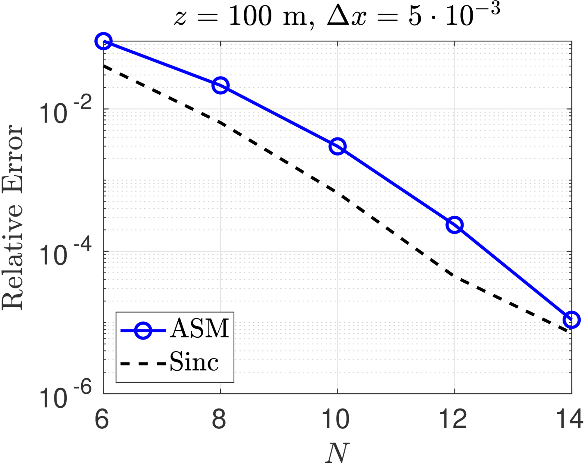
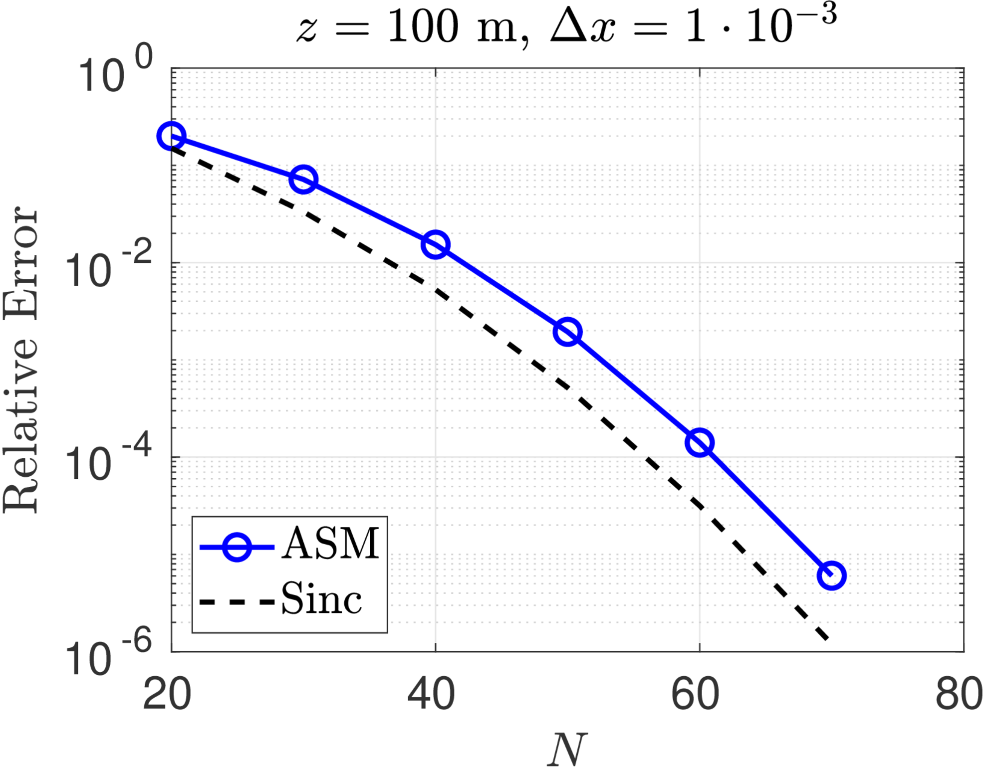
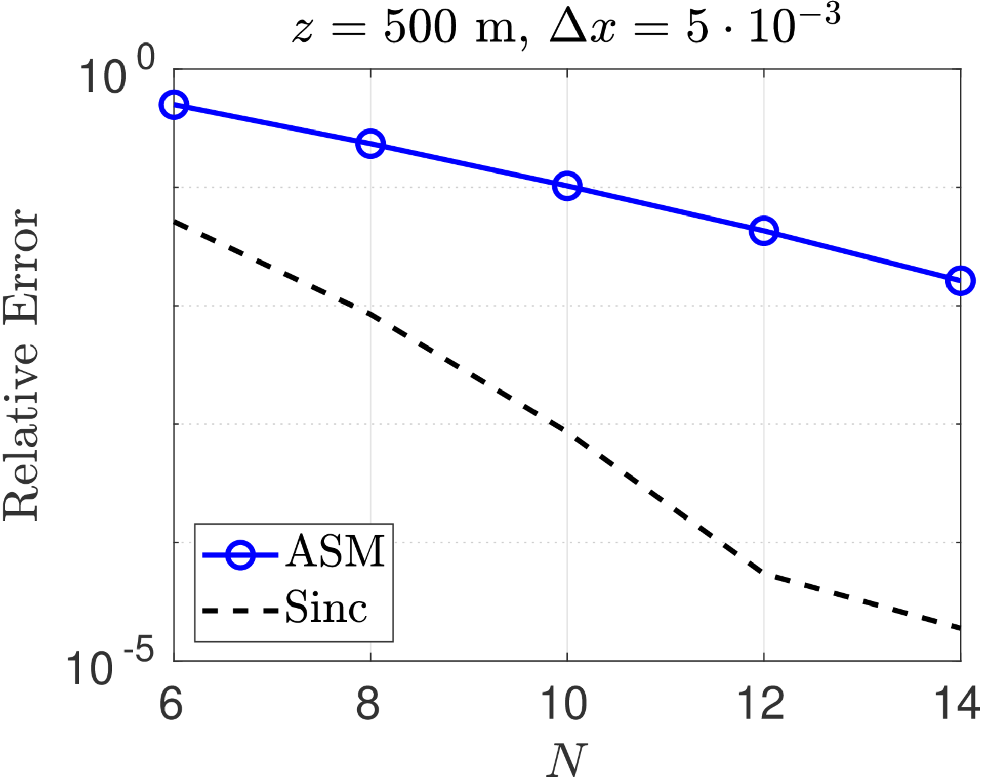
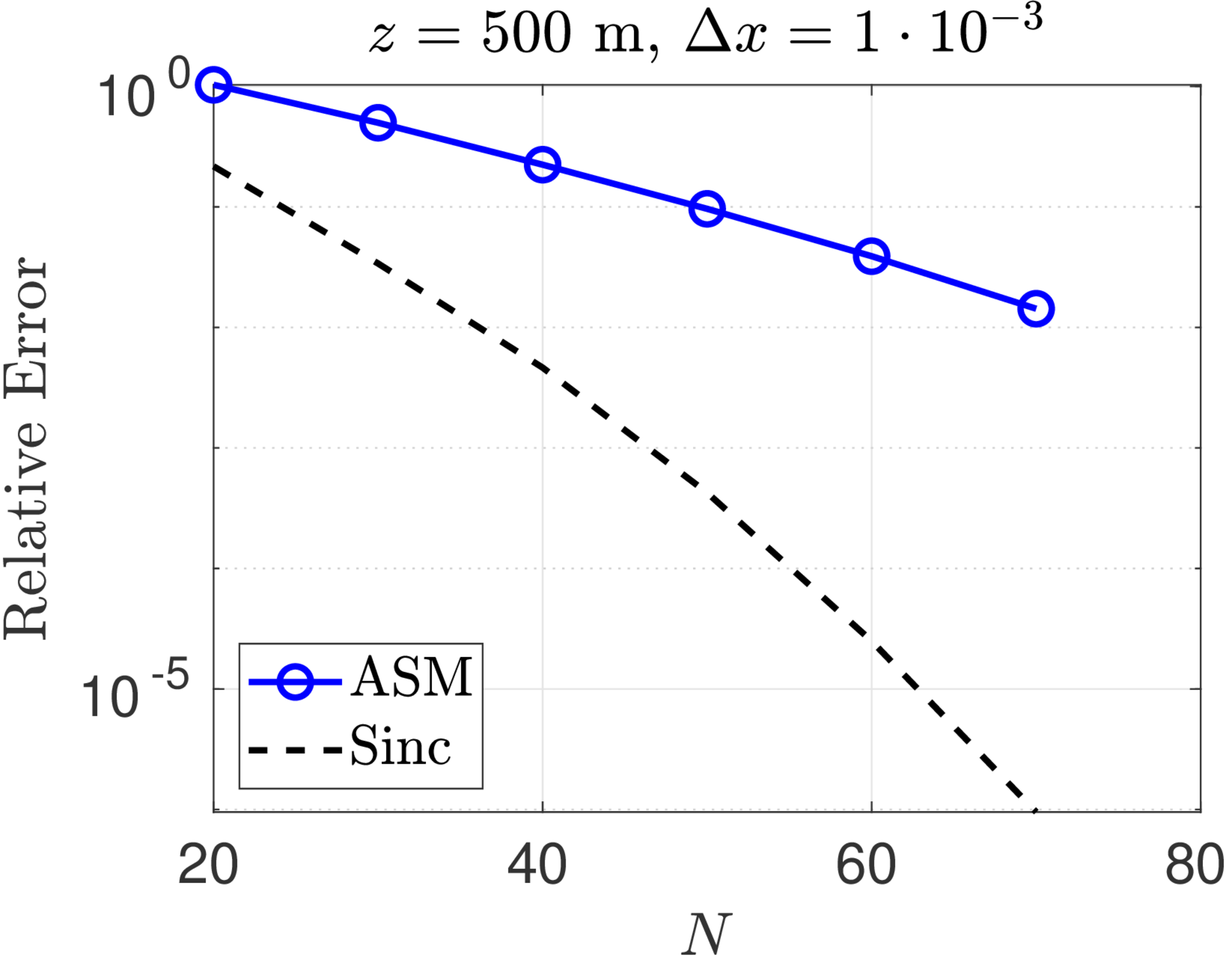
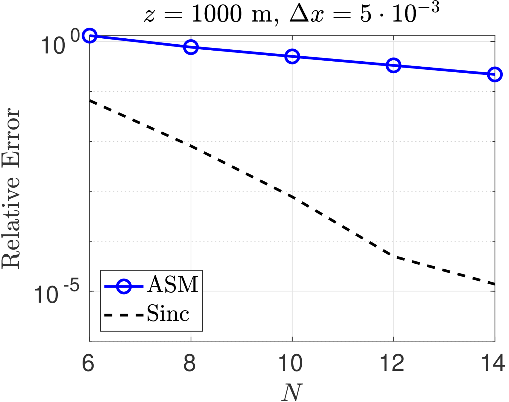
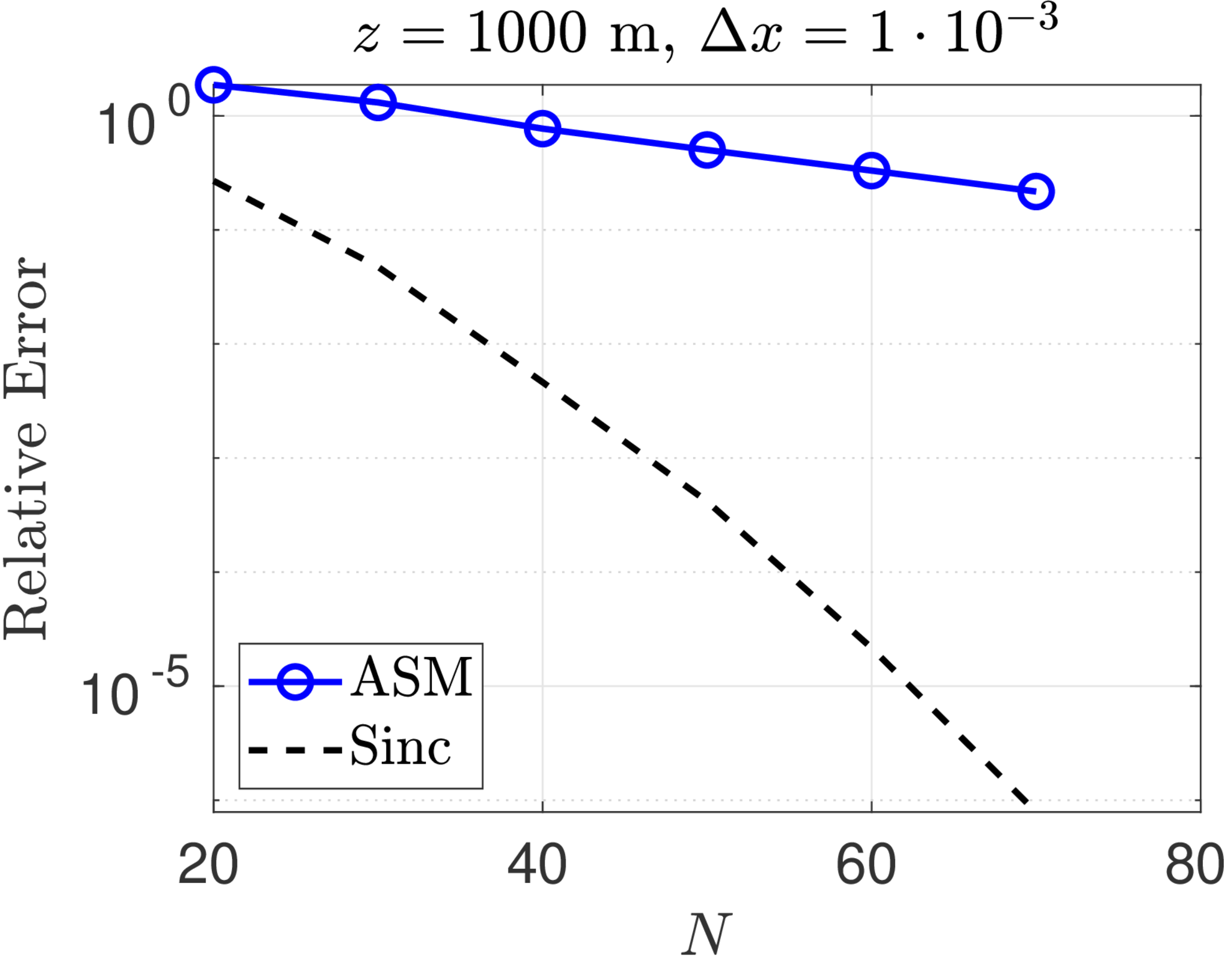
Figure 1 shows convergence plots for the sinc method and the ASM for Fresnel diffraction of a Gaussian beam with wavelength $\lambda=1\,\mu\textrm{m}$ and beam radius $w_{0}=1\,\textrm{cm}$ . Three different propagation distances, $z\in\{100,\,500,\,1000\}$ m, and two sample spacings, $\Delta x\in\{1\cdot 10^{-3},\,5\cdot 10^{-3}\}$ m, were chosen for this study. The exact solution is computed at every point of an observation plane grid of $N\times N$ points and the $2$ -norm relative error is computed for both the ASM and the sinc numerical solutions. The errors for the ASM are competitive with (but still greater than) the sinc method at shorter propagation distances. As the analysis predicted, however, ASM performs worse at longer distances. On the other hand, for fixed $\Delta x$ , the convergence of the sinc method is almost identical for all propagation distances.

5.2 Circular aperture

Next, we consider a diffraction problem for a circular aperture using both the Fresnel and Rayleigh-Sommerfeld integrals. Unfortunately, in this case, there is no closed-form solution, even for the simpler Fresnel case.

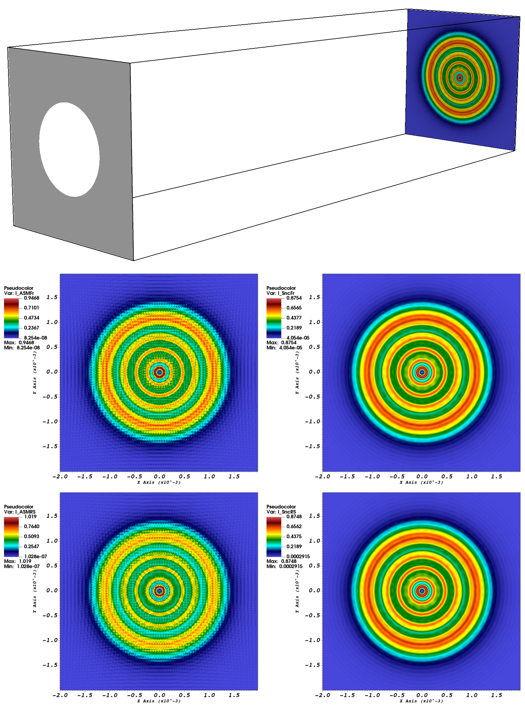
The problem setup is as follows (all units are in meters). The field in the source plane is given by

u(x,y,z)=A\text{circ}\left(\frac{r}{r_{0}}\right)\frac{e^{ik\sqrt{(x-x_{0})^{2}+(y-y_{0})^{2}+(z-z_{0})^{2}}}}{\sqrt{(x-x_{0})^{2}+(y-y_{0})^{2}+(z-z_{0})^{2}}},\qquad\text{circ}(r)\coloneqq\begin{cases}1,&r\leq 1,\\ 0,&\textrm{otherwise},\end{cases}

(79)

where the wavelength $\lambda=10\,\mu\textrm{m}$ , $r=\sqrt{x^{2}+y^{2}}$ , $r_{0}=10^{-3}$ is the circular aperture radius, $A=3\cdot 10^{-2}$ is the source amplitude, and $(x_{0},y_{0},z_{0})=(0,0,-3\cdot 10^{-2})$ so that the source is placed slightly behind the an opaque screen at $z=0$ . The source $u$ is evaluated over a planar grid with $N\times N$ points for $(x,y)\in[-2\cdot 10^{-3},2\cdot 10^{-3}]^{2}$ , with $N=400$ in all cases, which we then propagate using each of the diffraction integrals (2) and (1).

Figure 2 shows irradiance patterns ( $|U|^{2}$ ) for Fresnel and Rayleigh-Sommerfeld diffraction, computed with the ASM and sinc methods, for a circular aperture over a uniform $N\times N$ planar grid at $z=0.015$ . Because the source field of the aperture problem is discontinuous, we expect that both the Fourier series and sinc series approximations will suffer from the Gibbs phenomenon. However, recalling the discussion of group velocity in Section 3.1, the highest frequency modes are quickly dispersed off to infinity so that the solution becomes smoother at longer propagation distances. This behavior is evident in the solution given by the sinc method; on the other hand, ASM retains all the high frequency oscillations, which are clearly visible in the pseudocolor plots of both the Fresnel and Rayleigh-Sommerfeld cases, regardless of propagation distance. (Pseudocolor plots were generated using the visualization software VisIt [18].)

6 Conclusion

We presented a method based on sinc approximations to compute Rayleigh-Sommefeld (RS) and Fresnel diffraction integrals. We compared our approach with the standard method used to evaluate these optical wave propagation integrals, the angular spectrum method (ASM), and we showed that the ASM introduces artificial periodicity into the domain. The ASM’s artificial periodicity, in turn, leads to errors in the optical fields which grow as the propagation distance increases. On the other hand, our sinc-based approach does not impose artifical periodic boundary conditions and instead correctly disperses transverse modes to infinity. Additionally, unlike the ASM, the sinc method preserves the bandwidth of the underlying convolution and the accuracy of the propagated field depends only on the approximation accuracy of the source field and is independent of wavelength, propagation distance, and observation plane discretization. Like the ASM, our sinc method can also be formulated as a discrete convolution over uniform grids and can thus be computed using FFTs. When the Fresnel number is large, only a few terms of the sinc quadrature are necessary to achieve a prescribed error tolerance; in this case, the sinc-based approach simplifies to an even faster $O(N)$ algorithm. For the Fresnel case, the set of sinc integration weights was given analytically and numerical results confirmed that the sinc approach achieves high-order accuracy for both short-range and long-range propagation. Similar results were obtained with the sinc-based method for RS diffraction through a circular aperture even though in that case the sinc integration weights were computed numerically. As expected, for a fixed discretization resolution, the ASM error confirmed that the solution deteriorates with increasing propagation distance.

Acknowledgements

This work was supported by the Air Force Office of Scientific Research [grant number 20RDCOR016].

Disclosures

Approved for public release; distribution is unlimited. Public Affairs release approval number AFRL-2021-3954.

References

Sherman [1967] G. C. Sherman, Integral-transform formulation of diffraction theory, JOSA 57 (1967) 1490–1498.
Shewell and Wolf [1968] J. Shewell, E. Wolf, Inverse diffraction and a new reciprocity theorem, JOSA 58 (1968) 1596–1603.
Goodman [1996] J. Goodman, Introduction to Fourier Optics, Electrical Engineering Series, McGraw-Hill, 1996.
Schmidt [2010] J. D. Schmidt, Numerical Simulation of Optical Wave Propagation with Examples in MATLAB, SPIE, 2010.
Voelz [2011] D. G. Voelz, Computational Fourier Optics: a MATLAB Tutorial, SPIE, 2011.
Matsushima and Shimobaba [2009] K. Matsushima, T. Shimobaba, Band-Limited Angular Spectrum Method for Numerical Simulation of Free-Space Propagation in Far and Near Fields, Optics Express 17 (2009) 19662–19673.
Zhang et al. [2020] W. Zhang, H. Zhang, C. J. R. Sheppard, G. Jin, Analysis of numerical diffraction calculation methods: from the perspective of phase space optics and the sampling theorem, JOSA A 37 (2020) 1748–1766.
Borel [1897] E. Borel, Sur l’interpolation, CR Acad. Sci. Paris 124 (1897) 673–676.
Whittaker [1915] E. T. Whittaker, On the Functions which are represented by the Expansions of the Interpolation-Theory, Proceedings of the Royal Society of Edinburgh 35 (1915) 181–194.
Stenger [2012] F. Stenger, Numerical methods based on Sinc and analytic functions, volume 20, Springer Science & Business Media, 2012.
Debnath and Mikusinski [2005] L. Debnath, P. Mikusinski, Introduction to Hilbert spaces with applications, Academic press, 2005.
Lalor [1968] É. Lalor, Conditions for the validity of the angular spectrum of plane waves, Journal of the Optical Society of America 58 (1968) 1235–1237.
Blackledge [2005] J. Blackledge, Digital Image Processing: Mathematical and Computational Methods, Woodhead Publishing Series in Electronic and Optical Materials, Elsevier Science, 2005.
Keefe et al. [2018] L. Keefe, I. Zilberter, T. J. Madden, When Parabolized Propagation Fails: A Matrix Square Root Propagator for EM Waves, in: Plasmadynamics and Lasers Conference, AIAA, 2018. doi:10.2514/6.2018-3113.
Waldvogel [2006] J. Waldvogel, Fast construction of the Fejér and Clenshaw–Curtis quadrature rules, BIT Numerical Mathematics 46 (2006) 195–202.
Nascov and Logofătu [2009] V. Nascov, P. C. Logofătu, Fast computation algorithm for the Rayleigh-Sommerfeld diffraction formula using a type of scaled convolution, Applied Optics 48 (2009) 4310–4319.
Bailey and Swarztrauber [1991] D. H. Bailey, P. N. Swarztrauber, The fractional Fourier transform and applications, SIAM Review 33 (1991) 389–404.
Childs et al. [2012] H. Childs, E. Brugger, B. Whitlock, J. Meredith, S. Ahern, D. Pugmire, K. Biagas, M. Miller, C. Harrison, G. H. Weber, H. Krishnan, T. Fogal, A. Sanderson, C. Garth, E. W. Bethel, D. Camp, O. Rübel, M. Durant, J. M. Favre, P. Navrátil, VisIt: An End-User Tool For Visualizing and Analyzing Very Large Data, in: High Performance Visualization–Enabling Extreme-Scale Scientific Insight, 2012, pp. 357–372.