This paper was converted on www.awesomepapers.org from LaTeX by an anonymous user.
Want to know more? Visit the Converter page.

Diffusion Approximations for Expert Opinions in a Financial Market with Gaussian Drift

Jörn Sass, Dorothee Westphal111Department of Mathematics, Technische Universität Kaiserslautern,
P.O. Box 3049, 67653 Kaiserslautern, Germany; westphal@mathematik.uni-kl.de
 and Ralf Wunderlich222Institute of Mathematics, Brandenburg University of Technology Cottbus-Senftenberg,
P.O. Box 101344, 03013 Cottbus, Germany; ralf.wunderlich@b-tu.de
Department of Mathematics, Technische Universität Kaiserslautern,
P.O. Box 3049, 67653 Kaiserslautern, Germany; sass@mathematik.uni-kl.de
(March 5, 2020)
Abstract

This paper investigates a financial market where returns depend on an unobservable Gaussian drift process. While the observation of returns yields information about the underlying drift, we also incorporate discrete-time expert opinions as an external source of information.

For estimating the hidden drift it is crucial to consider the conditional distribution of the drift given the available observations, the so-called filter. For an investor observing both the return process and the discrete-time expert opinions, we investigate in detail the asymptotic behavior of the filter as the frequency of the arrival of expert opinions tends to infinity. In our setting, a higher frequency of expert opinions comes at the cost of accuracy, meaning that as the frequency of expert opinions increases, the variance of expert opinions becomes larger. We consider a model where information dates are deterministic and equidistant and another model where the information dates arrive randomly as the jump times of a Poisson process. In both cases we derive limit theorems stating that the information obtained from observing the discrete-time expert opinions is asymptotically the same as that from observing a certain diffusion process which can be interpreted as a continuous-time expert.

We use our limit theorems to derive so-called diffusion approximations of the filter for high-frequency discrete-time expert opinions. These diffusion approximations are extremely helpful for deriving simplified approximate solutions of utility maximization problems.


Keywords: Diffusion approximations, Kalman filter, Ornstein–Uhlenbeck process, Expert opinions, Portfolio optimization, Partial information

2010 Mathematics Subject Classification: Primary 91G10; Secondary 93E11, 93E20, 60F25.

1 Introduction

Optimal trading strategies in dynamic portfolio optimization problems depend crucially on the drift of the underlying asset price processes. However, drift parameters are notoriously difficult to estimate from historical asset price data. Drift processes tend to fluctuate randomly over time and even if they were constant, long time series would be needed to estimate this parameter with a satisfactory degree of precision. Typically, drift effects are overshadowed by volatility. For these reasons, practitioners also incorporate external sources of information such as news, company reports, ratings or their own intuitive views when determining optimal portfolio strategies. These outside sources of information are called expert opinions. In the context of the classical one-period Markowitz model this leads to the well-known Black–Litterman approach, where return predictions are improved by means of views formulated by securities analysts, see Black and Litterman [3].

In this paper we consider a financial market where returns depend on an underlying drift process which is unobservable due to additional noise coming from a Brownian motion. The general setting has already been studied in Gabih et al. [11] for a market with only one risky asset and in Sass et al. [23] for markets with an arbitrary number of stocks. The ability to choose good trading strategies depends on how well the unobserved drift can be estimated. For estimating the hidden drift we consider the conditional distribution of the drift given the available observations, the so-called filter. The best estimate for the hidden drift process in a mean-square sense is the conditional mean of the drift given the available information. A measure for the goodness of this estimator is its conditional covariance matrix. In our setting, the filter is completely characterized by conditional mean and conditional covariance matrix since we deal with Gaussian distributions.

For investors who observe only the return process, the filter is the classical Kalman filter, see for example Liptser and Shiryaev [19]. An additional source of information is provided by expert opinions which we model as unbiased drift estimates arriving at discrete points in time. Investors who, in addition to observing the return process, have access to these expert opinions update their current drift estimates at each arrival time. These updates decrease the conditional covariance, hence they yield better estimates. This can be seen as a continuous-time version of the above mentioned static Black–Litterman approach.

We investigate in detail an investor who observes both the return process and the discrete-time expert opinions and study the asymptotic behavior of the filter when the frequency of the arrival of expert opinions tends to infinity. Sass et al. [23] and Gabih et al. [12] already addressed expert opinions which are independent of the arrival frequency and which have some minimal level of accuracy characterized by bounded covariances. In that setting, the conditional covariance of the drift estimate goes to zero as the arrival frequency goes to infinity. This implies that the conditional mean converges to the true drift process, i.e. in the limit investors have full information about the drift. Here, we study a different situation in which a higher frequency of expert opinions is only available at the cost of accuracy of the single expert opinions. In other words, as the frequency of expert opinions increases, the variance of expert opinions becomes larger. On the one hand, this assumption ensures that it is not possible for investors to gain arbitrarily much information in a fixed time interval. On the other hand, it enables us to derive a certain asymptotic behavior that yields a reasonable approximation of the filter for the investor who observes a certain, fixed number of discrete-time expert opinions. We consider two different situations, one with deterministic equidistant information dates and one with information dates that arrive randomly as the jump times of a Poisson process. For properly scaled variance of expert opinions that grows linearly with the arrival frequency we prove Lp\mathrm{L}\rule{0.0pt}{7.5pt}^{p}-convergence of the conditional mean and conditional covariance matrices as the frequency of information dates goes to infinity. Our limit theorems imply that the information obtained from observing the discrete-time expert opinions is asymptotically the same as that from observing a certain diffusion process having the same drift as the return process. That process can be interpreted as a continuous-time expert who permanently delivers noisy information about the drift.

Our limit theorems allow us to derive approximations of the filter for high-frequency discrete-time expert opinions which we call diffusion approximations. These are useful since the limiting filter is easy to compute whereas the updates for the discrete-time expert opinions lead to a computationally involved filter. This is extremely helpful for deriving simplified approximate solutions of utility maximization problems. We apply our diffusion approximations to a portfolio optimization problem with logarithmic utility. Numerical simulations show that the approximation is very accurate even for a small number of expert opinions. Our rigorous Lp\mathrm{L}\rule{0.0pt}{7.5pt}^{p}-convergence results of the filters however also allow to derive convergence of the value function in the more complicated problem with power utility, see Remark 5.5.

The idea of a continuous-time expert is in line with Davis and Lleo [7] who study an approach called “Black–Litterman in Continuous Time” (BLCT). Our results show how the BLCT model can be obtained as a limit of BLCT models with discrete-time experts. First papers addressing BLCT are Frey et al. [9, 10] who consider an HMM for the drift and expert opinions arriving at the jump times of a Poisson process.

Convergence of the discrete-time Kalman filter to the continuous-time equivalent has been addressed in the literature, e.g. by Salgado et al. [22] or Aalto [1] for the case of deterministic information dates. Our results for that case however do not follow directly from these convergence results. The reason is that in our case a suitable continuous-time expert has to be constructed first. The discrete-time expert opinions are then not simply a discretization of the continuous-time expert. We assume that they are noisy observations of the true drift process where the noise term is correlated with the Brownian motion in the diffusion that forms the continuous-time expert. Contrary to [1, 22] we also obtain convergence results for the case where the discrete expert opinions arrive at random time points rather than on an equidistant time grid.

Coquet et al. [6] consider weak convergence of filtrations which allows to prove convergence of conditional expectations in a quite general setting. However, their results do not directly apply to our situation since the approximating sequence of filtrations in our case is not included in the limit filtration.

In the literature, diffusion approximations also appear in other contexts. They are well-known in operations research and actuarial mathematics. The basic idea is to replace a complicated stochastic process by an appropriate diffusion process which is analytically more tractable than the original process. The approach is comparable with the normal approximation of sums of random variables by the Central Limit Theorem. When looking at these sums as stochastic processes or random walks the well-known Donsker Theorem leads to an approximation by a Brownian motion.

For an introduction to diffusion approximations based on the theory of weak convergence and applications to queueing systems in heavy traffic we refer to the survey article by Glynn [13]. In risk theory the application of diffusion approximations for computing ruin probabilities goes back to Iglehart [15]. We also refer to Grandell [14, Sec. 1.2], Schmidli [24, Sec. 5.10 and 6.5] and Asmussen and Albrecher [2, Sec. V.5] as well as the references therein. Starting point is the classical Cramér–Lundberg model where the cumulated claim sizes and finally the surplus of an insurance company are modeled by a compound Poisson process. For a high intensity of the claim arrivals and small claim sizes the latter can be approximated by a Brownian motion with drift. This results from the corresponding weak convergence of the properly scaled compound Poisson processes to a Brownian motion as the intensity tends to infinity. However, these classical results for compound Poisson processes cannot be applied directly to our problem. Here, the jumps of the filter processes do not constitute a sequence of i.i.d. random variables as in the compound Poisson case. Due to the Bayesian updating of the filter at the information dates the jump size distribution depends on the value of the filter at that time. This requires special techniques for proving limit theorems from which the diffusion approximations can be derived. To the best of our knowledge these techniques constitute a new contribution to the literature.

The paper is organized as follows. In Section 2 we introduce the model for our financial market including expert opinions and define different information regimes for investors with different sources of information. For each of those information regimes, we state the dynamics of the corresponding conditional mean and conditional covariance matrix. Section 3 investigates the situation where the discrete-time expert opinions arrive at deterministic equidistant time points. For an investor observing returns and discrete-time expert opinions we show convergence of the corresponding conditional mean and conditional covariance matrix to those of an investor observing the returns and the continuous-time expert. In Section 4 we prove analogous results for the situation where the time points at which expert opinions arrive are not deterministic time points but jump times of a standard Poisson process, i.e. with exponentially distributed waiting times between information dates. For the conditional mean we can then use a representation involving a Poisson random measure. When letting the intensity of the Poisson process go to infinity, we prove convergence to the same limiting filter as in the case with deterministic information dates. Section 5 provides an application of the convergence results to a utility maximization problem. For investors who maximize expected logarithmic utility of terminal wealth the optimal trading strategy depends on the conditional mean of the drift and the corresponding optimal terminal wealth is a functional of the conditional covariance matrices. That is why the convergence results from Sections 3 and 4 carry over to convergence of the corresponding value functions. Section 6 provides simulations and numerical calculations to illustrate our theoretical results. In Appendix A we collect some auxiliary results needed for the proofs of our main theorems. Appendix B gives the proofs of Theorems 3.2 and 3.3 and Appendix C those of Theorems 4.6 and 4.7.

Notation:

Throughout this paper, we use the notation IdI_{d} for the identity matrix in d×d\mathbb{R}^{d\times d}. For a symmetric and positive-semidefinite matrix Ad×dA\in\mathbb{R}^{d\times d} we call a symmetric and positive-semidefinite matrix Bd×dB\in\mathbb{R}^{d\times d} the square root of AA if B2=AB^{2}=A. The square root is unique and will be denoted by A12A^{\frac{1}{2}}. Unless stated otherwise, whenever AA is a matrix, A\lVert A\rVert denotes the spectral norm of AA.

2 Market Model and Filtering

2.1 Financial Market Model

We consider a financial market with one risk-free and multiple risky assets. The basic model is the same as in Sass et al. [23]. In the following, we denote by T>0T>0 a finite investment horizon and fix a filtered probability space (Ω,𝒢,𝔾,)(\Omega,\mathcal{G},\mathbb{G},\mathbb{P}) where the filtration 𝔾=(𝒢t)t[0,T]\mathbb{G}=(\mathcal{G}_{t})_{t\in[0,T]} satisfies the usual conditions. All processes are assumed to be 𝔾\mathbb{G}-adapted. The market consists of one risk-free bond with constant deterministic interest rate rr\in\mathbb{R}, and dd risky assets such that the dd-dimensional return process follows the stochastic differential equation

dRt=μtdt+σRdWtR.\mathrm{d}R_{t}=\mu_{t}\,\mathrm{d}t+\sigma_{R}\,\mathrm{d}W^{R}_{t}.

Here WR=(WtR)t[0,T]W^{R}=(W^{R}_{t})_{t\in[0,T]} is an mm-dimensional Brownian motion with mdm\geq d and we assume that σRd×m\sigma_{R}\in\mathbb{R}^{d\times m} has full rank. The drift μ\mu is an Ornstein–Uhlenbeck process and follows the dynamics

dμt=α(δμt)dt+βdBt,\mathrm{d}\mu_{t}=\alpha(\delta-\mu_{t})\,\mathrm{d}t+\beta\,\mathrm{d}B_{t},

where α\alpha and βd×d\beta\in\mathbb{R}^{d\times d}, δd\delta\in\mathbb{R}^{d} and B=(Bt)t[0,T]B=(B_{t})_{t\in[0,T]} is a dd-dimensional Brownian motion independent of WRW^{R}. We assume that α\alpha is a symmetric and positive-definite matrix to ensure that expectation and covariance of the drift process stay bounded and the drift process becomes asymptotically stationary. This is reasonable from an economic point of view. The initial drift μ0\mu_{0} is multivariate normally distributed, μ0𝒩(m0,Σ0)\mu_{0}\sim\mathcal{N}(m_{0},\Sigma_{0}), for some m0dm_{0}\in\mathbb{R}^{d} and some Σ0d×d\Sigma_{0}\in\mathbb{R}^{d\times d} which is symmetric and positive semidefinite. We assume that μ0\mu_{0} is independent of BB and WRW^{R}. We denote mt:=𝔼[μt]m_{t}:=\operatorname{\mathbb{E}}[\mu_{t}] and Σt:=cov(μt)\Sigma_{t}:=\operatorname{cov}(\mu_{t}).

Investors in this market know the model parameters and are able to observe the return process RR. They neither observe the underlying drift process μ\mu nor the Brownian motion WRW^{R}. However, information about μ\mu can be drawn from observing RR. Additionally, we include expert opinions in our model. These expert opinions arrive at discrete time points and give an unbiased estimate of the state of the drift at that time point. Let (Tk)kI(T_{k})_{k\in I} be an increasing sequence with values in (0,T](0,T], where we allow for index sets I=I=\mathbb{N} or I={1,,N}I=\{1,\dots,N\} for some NN\in\mathbb{N}. The TkT_{k}, kIk\in I, are the time points at which expert opinions arrive. For the sake of convenience we also write T0=0T_{0}=0 although there is not necessarily an expert opinion arriving at time zero.

The expert view at time TkT_{k} is modelled as an d\mathbb{R}^{d}-valued random vector

Zk=μTk+(Γk)12εk,Z_{k}=\mu_{T_{k}}+(\Gamma_{k})^{\frac{1}{2}}\varepsilon_{k},

where the matrix Γkd×d\Gamma_{k}\in\mathbb{R}^{d\times d} is symmetric and positive definite and εk\varepsilon_{k} is multivariate 𝒩(0,Id)\mathcal{N}(0,I_{d})-distributed. We assume that the sequence of εk\varepsilon_{k} is independent and also that it is independent of both μ0\mu_{0} and the Brownian motions BB and WRW^{R}. Note that, given μTk\mu_{T_{k}}, the expert opinion ZkZ_{k} is multivariate 𝒩(μTk,Γk)\mathcal{N}(\mu_{T_{k}},\Gamma_{k})-distributed. That means that the expert view at time TkT_{k} gives an unbiased estimate of the state of the drift at that time. The matrix Γk\Gamma_{k} reflects the reliability of the expert.

Note that the time points TkT_{k} do not need to be deterministic. However, we impose the additional assumption that the sequence (Tk)kI(T_{k})_{k\in I} is independent of the (εk)kI(\varepsilon_{k})_{k\in I} and also of the Brownian motions in the market and of μ0\mu_{0}. This essentially says that the timing of information dates carries no additional information about the drift μ\mu. Nevertheless, information on the sequence (Tk)kI(T_{k})_{k\in I} may be important for optimal portfolio decisions. In the next sections we consider on the one hand the situation with deterministic information dates and on the other hand a case where information dates are the jump times of a Poisson process.

It is possible to allow relative expert views in the sense that an expert may give an estimate for the difference in drift of two stocks instead of absolute views. See Schöttle et al. [25] for how to switch between these two models for expert opinions by means of a pick matrix.

Our main results in Sections 3 and 4 address the question how to obtain rigorous convergence results when the number of information dates increases. We will show that, for certain sequences of expert opinions, the information drawn from these expert opinions, expressed by the filter, is for a large number of expert opinions essentially the same as the information one gets from observing yet another diffusion process. This diffusion process can then be interpreted as an expert who gives a continuous-time estimation about the state of the drift. Let this estimate be given by the diffusion process

dJt=μtdt+σJdWtJ,\mathrm{d}J_{t}=\mu_{t}\,\mathrm{d}t+\sigma_{J}\,\mathrm{d}W^{J}_{t}, (2.1)

where WJW^{J} is an ll-dimensional Brownian motion with ldl\geq d that is independent of all other Brownian motions in the model and of the information dates TkT_{k}. The matrix σJd×l\sigma_{J}\in\mathbb{R}^{d\times l} has full rank equal to dd.

2.2 Filtering for Different Information Regimes

For an investor in the financial market defined above, the ability to choose good trading strategies is based heavily on which information is available about the unknown drift process μ\mu. To be able to assess the value of information coming from observing expert opinions, we consider various types of investors with different sources of information. This follows the approach in Gabih et al. [11] and in Sass et al. [23]. The information available to an investor can be described by the investor filtration 𝔽H=(tH)t[0,T]\mathbb{F}^{H}=(\mathcal{F}^{H}_{t})_{t\in[0,T]} where HH serves as a placeholder for the various information regimes. We work with filtrations that are augmented by 𝒩\mathcal{N}_{\mathbb{P}}, the set of null sets under measure \mathbb{P}. We consider the cases

𝔽R\displaystyle\mathbb{F}^{R} =(tR)t[0,T]\displaystyle=(\mathcal{F}^{R}_{t})_{t\in[0,T]} where tR=σ((Rs)s[0,t])σ(𝒩),\displaystyle\text{ where }\mathcal{F}^{R}_{t}=\sigma((R_{s})_{s\in[0,t]})\vee\sigma(\mathcal{N}_{\mathbb{P}}),
𝔽Z\displaystyle\mathbb{F}^{Z} =(tZ)t[0,T]\displaystyle=(\mathcal{F}^{Z}_{t})_{t\in[0,T]} where tZ=σ((Rs)s[0,t])σ((Tk,Zk)Tkt)σ(𝒩),\displaystyle\text{ where }\mathcal{F}^{Z}_{t}=\sigma((R_{s})_{s\in[0,t]})\vee\sigma((T_{k},Z_{k})_{T_{k}\leq t})\vee\sigma(\mathcal{N}_{\mathbb{P}}),
𝔽J\displaystyle\mathbb{F}^{J} =(tJ)t[0,T]\displaystyle=(\mathcal{F}^{J}_{t})_{t\in[0,T]} where tJ=σ((Rs)s[0,t])σ((Js)s[0,t])σ(𝒩),\displaystyle\text{ where }\mathcal{F}^{J}_{t}=\sigma((R_{s})_{s\in[0,t]})\vee\sigma((J_{s})_{s\in[0,t]})\vee\sigma(\mathcal{N}_{\mathbb{P}}),
𝔽F\displaystyle\mathbb{F}^{F} =(tF)t[0,T]\displaystyle=(\mathcal{F}^{F}_{t})_{t\in[0,T]} where tF=σ((Rs)s[0,t])σ((μs)s[0,t])σ(𝒩).\displaystyle\text{ where }\mathcal{F}^{F}_{t}=\sigma((R_{s})_{s\in[0,t]})\vee\sigma((\mu_{s})_{s\in[0,t]})\vee\sigma(\mathcal{N}_{\mathbb{P}}).

When speaking of the HH-investor we mean the investor with investor filtration 𝔽H=(tH)t[0,T]\mathbb{F}^{H}=(\mathcal{F}^{H}_{t})_{t\in[0,T]}, H{R,Z,J,F}H\in\{R,Z,J,F\}. Note that the RR-investor observes only the return process RR, the ZZ-investor combines the information from observing the return process and the discrete-time expert opinions ZkZ_{k}, and the JJ-investor observes the return process and the continuous-time expert JJ. The FF-investor has full information about the drift in the sense that she can observe the drift process directly. This case is included as a benchmark.

As already mentioned, the investors in our financial market make trading decisions based on available information about the drift process μ\mu. Only the FF-investor can observe the drift, the other investors have to estimate it. The conditional distribution of the drift under partial information is called the filter. In the mean-square sense, an optimal estimator for the drift at time tt given the available information is then the conditional mean mtH:=𝔼[μt|tH]m^{H}_{t}:=\operatorname{\mathbb{E}}[\mu_{t}\,|\,\mathcal{F}^{H}_{t}]. How close this estimator is to the true state of the drift can be assessed by looking at the corresponding conditional covariance matrix

QtH:=𝔼[(μtmtH)(μtmtH)|tH].Q^{H}_{t}:=\operatorname{\mathbb{E}}\bigl{[}(\mu_{t}-m^{H}_{t})(\mu_{t}-m^{H}_{t})^{\top}\,\big{|}\,\mathcal{F}^{H}_{t}\bigr{]}.

Note that since we deal with Gaussian distributions here, the filter is also Gaussian and completely characterized by conditional mean and conditional covariance matrix. In the next sections we investigate the behavior of the filter for a ZZ-investor with access to an increasing number of expert opinions. For this purpose, we state in the following the dynamics of the filters for the various investors defined above. For the RR-investor, we are in the setting of the well-known Kalman filter.

Lemma 2.1.

The filter of the RR-investor is Gaussian. The conditional mean mRm^{R} follows the dynamics

dmtR=α(δmtR)dt+QtR(σRσR)1(dRtmtRdt),\mathrm{d}m^{R}_{t}=\alpha(\delta-m^{R}_{t})\,\mathrm{d}t+Q^{R}_{t}(\sigma_{R}\sigma_{R}^{\top})^{-1}(\mathrm{d}R_{t}-m^{R}_{t}\,\mathrm{d}t),

where QRQ^{R} is the solution of the ordinary Riccati differential equation

ddtQtR=αQtRQtRα+ββQtR(σRσR)1QtR.\frac{\mathrm{d}}{\mathrm{d}t}Q^{R}_{t}=-\alpha Q^{R}_{t}-Q^{R}_{t}\alpha+\beta\beta^{\top}-Q^{R}_{t}(\sigma_{R}\sigma_{R}^{\top})^{-1}Q^{R}_{t}.

The initial values are m0R=m0m^{R}_{0}=m_{0} and Q0R=Σ0Q^{R}_{0}=\Sigma_{0}.

This lemma follows directly from the Kalman filter theory, see for example Theorem 10.3 of Liptser and Shiryaev [19]. Note that QtRQ^{R}_{t} follows an ordinary differential equation, called Riccati equation, and is hence deterministic.

Next, we consider the JJ-investor who observes the diffusion processes RR and JJ.

Lemma 2.2.

The filter of the JJ-investor is Gaussian. The conditional mean mJm^{J} follows the dynamics

dmtJ=α(δmtJ)dt+QtJ((σRσR)1(σJσJ)1)(dRtmtJdtdJtmtJdt),\mathrm{d}m^{J}_{t}=\alpha(\delta-m^{J}_{t})\,\mathrm{d}t+Q^{J}_{t}\begin{pmatrix}(\sigma_{R}\sigma_{R}^{\top})^{-1}\\[2.84526pt] (\sigma_{J}\sigma_{J}^{\top})^{-1}\end{pmatrix}^{\top}\begin{pmatrix}\mathrm{d}R_{t}-m^{J}_{t}\,\mathrm{d}t\\[2.84526pt] \mathrm{d}J_{t}-m^{J}_{t}\,\mathrm{d}t\end{pmatrix},

where QJQ^{J} is the solution of the ordinary Riccati differential equation

ddtQtJ=αQtJQtJα+ββQtJ((σRσR)1+(σJσJ)1)QtJ\frac{\mathrm{d}}{\mathrm{d}t}Q^{J}_{t}=-\alpha Q^{J}_{t}-Q^{J}_{t}\alpha+\beta\beta^{\top}-Q^{J}_{t}\bigl{(}(\sigma_{R}\sigma_{R}^{\top})^{-1}+(\sigma_{J}\sigma_{J}^{\top})^{-1}\bigr{)}Q^{J}_{t} (2.2)

with m0J=m0m^{J}_{0}=m_{0} and Q0J=Σ0Q^{J}_{0}=\Sigma_{0}.

Proof.

First, note that the matrix (σRσR)1+(σJσJ)1d×d(\sigma_{R}\sigma_{R}^{\top})^{-1}+(\sigma_{J}\sigma_{J}^{\top})^{-1}\in\mathbb{R}^{d\times d} is symmetric and positive definite, and hence nonsingular. The distribution of the filter as well as the dynamics of mJm^{J} and QJQ^{J} then follow immediately from the Kalman filter theory, see again Theorem 10.3 in Liptser and Shiryaev [19]. ∎

Note that, just like in the case for the RR-investor, the conditional covariance matrix is deterministic.

Let us now come to the ZZ-investor. Recall that this investor observes the return process RR continuously in time and at (possibly random) information dates TkT_{k} the expert opinions ZkZ_{k}. We state the dynamics of mZm^{Z} and QZQ^{Z} in the following lemma.

Lemma 2.3.

Given a sequence of information dates TkT_{k}, the filter of the ZZ-investor is Gaussian. The dynamics of the conditional mean and conditional covariance matrix are given as follows:

  1. (i)

    Between the information dates TkT_{k} and Tk+1T_{k+1}, k0k\in\mathbb{N}_{0}, it holds

    dmtZ=α(δmtZ)dt+QtZ(σRσR)1(dRtmtZdt)\mathrm{d}m^{Z}_{t}=\alpha(\delta-m^{Z}_{t})\,\mathrm{d}t+Q^{Z}_{t}(\sigma_{R}\sigma_{R}^{\top})^{-1}(\mathrm{d}R_{t}-m^{Z}_{t}\,\mathrm{d}t)

    for t[Tk,Tk+1)t\in[T_{k},T_{k+1}), where QZQ^{Z} follows the ordinary Riccati differential equation

    ddtQtZ=αQtZQtZα+ββQtZ(σRσR)1QtZ\frac{\mathrm{d}}{\mathrm{d}t}Q^{Z}_{t}=-\alpha Q^{Z}_{t}-Q^{Z}_{t}\alpha+\beta\beta^{\top}-Q^{Z}_{t}(\sigma_{R}\sigma_{R}^{\top})^{-1}Q^{Z}_{t}

    for t[Tk,Tk+1)t\in[T_{k},T_{k+1}). The initial values are mTkZm^{Z}_{T_{k}} and QTkZQ^{Z}_{T_{k}}, respectively, with m0Z=m0m^{Z}_{0}=m_{0} and Q0Z=Σ0Q^{Z}_{0}=\Sigma_{0}.

  2. (ii)

    The update formulas at information dates TkT_{k}, kk\in\mathbb{N}, are

    mTkZ\displaystyle m^{Z}_{T_{k}} =ρk(QTkZ)mTkZ+(Idρk(QTkZ))Zk\displaystyle=\rho_{k}(Q^{Z}_{T_{k}-})m^{Z}_{T_{k}-}+\bigl{(}I_{d}-\rho_{k}(Q^{Z}_{T_{k}-})\bigr{)}Z_{k}
    =mTkZ+(Idρk(QTkZ))(ZkmTkZ)\displaystyle=m^{Z}_{T_{k}-}+\bigl{(}I_{d}-\rho_{k}(Q^{Z}_{T_{k}-})\bigr{)}\bigl{(}Z_{k}-m^{Z}_{T_{k}-}\bigr{)}

    and

    QTkZ\displaystyle Q^{Z}_{T_{k}} =ρk(QTkZ)QTkZ\displaystyle=\rho_{k}(Q^{Z}_{T_{k}-})Q^{Z}_{T_{k}-}
    =QTkZ+(ρk(QTkZ)Id)QTkZ,\displaystyle=Q^{Z}_{T_{k}-}+\bigl{(}\rho_{k}(Q^{Z}_{T_{k}-})-I_{d}\bigr{)}Q^{Z}_{T_{k}-},

    where ρk(Q)=Γk(Q+Γk)1\rho_{k}(Q)=\Gamma_{k}(Q+\Gamma_{k})^{-1}.

Proof.

For deterministic time points TkT_{k}, the above lemma is Lemma 2.3 of Sass et al. [23] where a detailed proof is given. For the more general case where the TkT_{k} need not be deterministic, recall that we have made the assumption that the sequence (Tk)kI(T_{k})_{k\in I} is independent of the other random variables in the market. In particular, (Tk)kI(T_{k})_{k\in I} and the drift process μ\mu are independent. Because of that, the dynamics of the conditional mean and conditional covariance matrix are the same as for deterministic information dates and we get the same update formulas, the only difference being that the update times might now be non-deterministic.

The Gaussian distribution of the filter between information dates follows as in the previous lemmas from the Kalman filter theory. The updates at information dates can be seen as a degenerate discrete-time Kalman filter. Hence, the distribution of the filter at information dates remains Gaussian after the Bayesian update. ∎

Note that the dynamics of mZm^{Z} and QZQ^{Z} between information dates are the same as for the RR-investor, see Lemma 2.1. The values at an information date TkT_{k} are obtained from a Bayesian update. If we have non-deterministic information dates TkT_{k} then in contrast to both the RR-investor and the JJ-investor, the conditional covariance matrices QZQ^{Z} of the ZZ-investor are non-deterministic since updates take place at random times.

In the proofs of our main results we repeatedly need to find upper bounds for various expressions that involve the conditional covariance matrices QJQ^{J} or QZQ^{Z}. A key tool is boundedness of these matrices. Here, it is useful to consider a partial ordering of symmetric matrices. For symmetric matrices A,Bd×dA,B\in\mathbb{R}^{d\times d} we write ABA\preceq B if BAB-A is positive semidefinite. Note that ABA\preceq B in particular implies that AB\lVert A\rVert\leq\lVert B\rVert.

Lemma 2.4.

For any sequence (Tk,Zk)kI(T_{k},Z_{k})_{k\in I} we have QtZQtRQ^{Z}_{t}\preceq Q^{R}_{t} and QtJQtRQ^{J}_{t}\preceq Q^{R}_{t} for all t0t\geq 0. In particular, there exists a constant CQ>0C_{Q}>0 such that

QtZCQandQtJCQ\lVert Q^{Z}_{t}\rVert\leq C_{Q}\quad\text{and}\quad\lVert Q^{J}_{t}\rVert\leq C_{Q}

for all t[0,T]t\in[0,T].

Proof.

Let (Tk,Zk)kI(T_{k},Z_{k})_{k\in I} be any sequence of expert opinions and (QtZ)t[0,T](Q^{Z}_{t})_{t\in[0,T]} the conditional covariance matrices of the corresponding filter. Every update decreases the covariance in the sense that QTkZQTkZQ^{Z}_{T_{k}}\preceq Q^{Z}_{T_{k}-}, see Proposition 2.2 in Sass et al. [23]. Also, if (Pt)t0(P_{t})_{t\geq 0} and (P~t)t0(\tilde{P}_{t})_{t\geq 0} are solutions of the same Riccati differential equation, where the initial values fulfill P0P~0P_{0}\preceq\tilde{P}_{0}, then PtP~tP_{t}\preceq\tilde{P}_{t} for all t0t\geq 0, see for example Theorem 10 in Kuc̆era [18]. Inductively, we can deduce that in our setting QtZQtRQ^{Z}_{t}\preceq Q^{R}_{t} for all t0t\geq 0. Also, one can show that QtJQtRQ^{J}_{t}\preceq Q^{R}_{t} for all t0t\geq 0 in analogy to the proof of Proposition 3.1 in Sass et al. [23]. The key idea for the proof is to use the fact that tRtJ\mathcal{F}^{R}_{t}\subseteq\mathcal{F}^{J}_{t} for all t0t\geq 0.

By Theorem 4.1 in Sass et al. [23] there exists a positive-semidefinite matrix QRQ^{R}_{\infty} such that

limtQtR=QR.\lim_{t\to\infty}Q^{R}_{t}=Q^{R}_{\infty}.

Hence, QtR\lVert Q^{R}_{t}\rVert is bounded by some constant CQ>0C_{Q}>0, and the claim follows. ∎

3 Diffusion Approximation of Filters for Deterministic Information Dates

In this section we investigate the asymptotic behavior of the filters for a ZZ-investor when the frequency of expert opinion arrivals goes to infinity. We consider first the case for deterministic and equidistant information dates. Therefore, let nn\in\mathbb{N} and Δn=Tn\Delta_{n}=\frac{T}{n}. Now assume that Tk=tkT_{k}=t_{k} for every k=1,,nk=1,\dots,n, where (tk)k=1,,n(t_{k})_{k=1,\dots,n} is the sequence of deterministic time points tk=kΔnt_{k}=k\Delta_{n}. So there are nn expert opinions that arrive equidistantly in the time interval [0,T][0,T], the distance between two information dates being Δn\Delta_{n}.

In the following, we deduce convergence results for both the conditional means and the conditional covariance matrices of the ZZ-investor when sending nn to infinity. Note that convergence of discrete-time filters is addressed in earlier papers, e.g. by Salgado et al. [22] or Aalto [1]. There, the authors show convergence of the discrete-time Kalman filter to the continuous-time equivalent. In Aalto [1] the discrete-time filter is based on discrete-time observations of the continuous-time observation process whereas in Salgado et al. [22] the authors approximate both the continuous-time signal and observation by discrete-time processes. Neither of these assumptions match our model for the discrete-time expert opinions which is why we need to prove convergence in the following.

We use an additional superscript nn to emphasize dependence on the number of expert opinions, writing for example (QtZ,n)t[0,T](Q^{Z,n}_{t})_{t\in[0,T]} for the conditional covariance matrix of the filter corresponding to these nn expert opinions. In Sass et al. [23] a convergence result is proven for the case where the expert opinions are of the form

Zk(n)=μtk(n)+(Γk(n))12εk(n)Z_{k}^{(n)}=\mu_{t^{(n)}_{k}}+(\Gamma_{k}^{(n)})^{\frac{1}{2}}\varepsilon_{k}^{(n)} (3.1)

with expert’s covariances Γk(n)\Gamma_{k}^{(n)} that are bounded for all nn\in\mathbb{N} and k=1,,nk=1,\dots,n, see Theorem 3.1 in Sass et al. [23]. There it is shown that under the assumption of bounded expert’s covariances it holds

limnQtZ,n=0\lim_{n\to\infty}\lVert Q^{Z,n}_{t}\rVert=0

for any t(0,T]t\in(0,T]. Since QtZ,nQ^{Z,n}_{t} is a measure for the goodness of the estimator mtZ,nm^{Z,n}_{t}, this means that the conditional mean of the ZZ-investor becomes an arbitrarily good estimator for the true state of the drift μt\mu_{t}. One can easily deduce that

limn𝔼[mtZ,nμt2]=0\lim_{n\to\infty}\operatorname{\mathbb{E}}\Bigl{[}\bigl{\lVert}m^{Z,n}_{t}-\mu_{t}\bigr{\rVert}^{2}\Bigr{]}=0

for any t(0,T]t\in(0,T]. Hence, the ZZ-investor essentially approximates the fully informed FF-investor.

This result heavily relies on the assumption that the expert covariances Γk(n)\Gamma_{k}^{(n)} are all bounded, meaning that there is some minimal level of reliability of the experts. Here, we study a different situation where more frequent expert opinions are only available at the cost of accuracy. In other words, we assume that, as Δn\Delta_{n} goes to zero, the variance of expert opinions Zk(n)Z_{k}^{(n)} increases. This is done for the purpose of approximating mZ,nm^{Z,n} and QZ,nQ^{Z,n} for large nn\in\mathbb{N} and large Γk(n)\Gamma_{k}^{(n)}. In the following we assume for the sake of simplicity that Γk(n)=Γ(n)\Gamma_{k}^{(n)}=\Gamma^{(n)} is not time-dependent. We then show that for properly scaled Γ(n)\Gamma^{(n)} which grows linearly in nn, the information obtained from observing the discrete-time expert opinions is asymptotically the same as that from observing another diffusion process. This will be the diffusion JJ already defined in (2.1).

Assumption 3.1.

Let (Tk(n))k=1,,n=(tk(n))k=1,,n(T_{k}^{(n)})_{k=1,\dots,n}=(t_{k}^{(n)})_{k=1,\dots,n} where tk(n)=kΔnt_{k}^{(n)}=k\Delta_{n} for k=1,,nk=1,\dots,n. Furthermore, let the experts’ covariance matrices be given by

Γk(n)=Γ(n)=1ΔnσJσJ\Gamma_{k}^{(n)}=\Gamma^{(n)}=\frac{1}{\Delta_{n}}\sigma_{J}\sigma_{J}^{\top}

for k=1,,nk=1,\dots,n. Further, we assume that in (3.1) the 𝒩(0,Id)\mathcal{N}(0,I_{d})-distributed random variables εk(n)\varepsilon_{k}^{(n)} are linked with the Brownian motion WJW^{J} from (2.1) via εk(n)=1Δntk(n)tk+1(n)dWsJ\varepsilon_{k}^{(n)}=\frac{1}{\sqrt{\Delta_{n}}}\int_{t_{k}^{(n)}}^{t_{k+1}^{(n)}}\mathrm{d}W^{J}_{s}, so that the expert opinions are given as

Zk(n)=μtk(n)+1ΔnσJtk(n)tk+1(n)dWsJZ^{(n)}_{k}=\mu_{t^{(n)}_{k}}+\frac{1}{\Delta_{n}}\sigma_{J}\int_{t^{(n)}_{k}}^{t^{(n)}_{k+1}}\mathrm{d}W^{J}_{s} (3.2)

for k=1,,nk=1,\dots,n.

Recall that the matrix σJd×l\sigma_{J}\in\mathbb{R}^{d\times l} is exactly the volatility of the diffusion process JJ with the dynamics

dJt=μtdt+σJdWtJ,\mathrm{d}J_{t}=\mu_{t}\,\mathrm{d}t+\sigma_{J}\,\mathrm{d}W^{J}_{t},

and that σJ\sigma_{J} has full rank. With Zk(n)Z^{(n)}_{k} as defined above the discrete-time expert opinions and the continuous-time expert JJ are obviously correlated. In fact, it holds

Zk(n)1Δntk(n)tk+1(n)dJs=1Δn(Jtk+1(n)Jtk(n)).Z^{(n)}_{k}\approx\frac{1}{\Delta_{n}}\int_{t^{(n)}_{k}}^{t^{(n)}_{k+1}}\mathrm{d}J_{s}=\frac{1}{\Delta_{n}}\Bigl{(}J_{t^{(n)}_{k+1}}-J_{t^{(n)}_{k}}\Bigr{)}.

Further, one can easily show by using Donsker’s Theorem that the piecewise constant process (J~t)t[0,T](\widetilde{J}_{t})_{t\in[0,T]}, defined by

J~t:=Δnk=1t/ΔnZk(n)\widetilde{J}_{t}:=\Delta_{n}\sum_{k=1}^{\lfloor t/\Delta_{n}\rfloor}Z_{k}^{(n)}

for all t[0,T]t\in[0,T], converges in distribution to JtJ_{t} as nn goes to infinity. For our main convergence results that are given in the following, we however require stronger notions of convergence.

The following theorem now states uniform convergence of QtZ,nQ^{Z,n}_{t} to QtJQ^{J}_{t} on [0,T][0,T] for nn going to infinity.

Theorem 3.2.

Under Assumption 3.1 there exists a constant KQ>0K_{Q}>0 such that

QtZ,nQtJKQΔn\bigl{\lVert}Q^{Z,n}_{t}-Q^{J}_{t}\bigr{\rVert}\leq K_{Q}\Delta_{n}

for all t[0,T]t\in[0,T]. In particular,

limnsupt[0,T]QtZ,nQtJ=0.\lim_{n\to\infty}\sup_{t\in[0,T]}\bigl{\lVert}Q^{Z,n}_{t}-Q^{J}_{t}\bigr{\rVert}=0.

The proof of Theorem 3.2 is given in Appendix B. It makes use of a discrete version of Gronwall’s Lemma for error accumulation, see Lemma A.1 in Appendix A.

Using the uniform convergence of the conditional covariance matrices QZ,nQ^{Z,n} to QJQ^{J} we can also deduce convergence of the corresponding conditional mean mZ,nm^{Z,n} to mJm^{J} in an Lp\mathrm{L}\rule{0.0pt}{7.5pt}^{p}-sense.

Theorem 3.3.

Let p[1,)p\in[1,\infty). Under Assumption 3.1 there exists a constant Km,p>0K_{m,p}>0 such that

𝔼[mtZ,nmtJp]Km,pΔnp/2\operatorname{\mathbb{E}}\Bigl{[}\bigl{\lVert}m^{Z,n}_{t}-m^{J}_{t}\bigr{\rVert}^{p}\Bigr{]}\leq K_{m,p}\Delta_{n}^{p/2}

for all t[0,T]t\in[0,T]. In particular,

limnsupt[0,T]𝔼[mtZ,nmtJp]=0.\lim_{n\to\infty}\sup_{t\in[0,T]}\operatorname{\mathbb{E}}\Bigl{[}\bigl{\lVert}m^{Z,n}_{t}-m^{J}_{t}\bigr{\rVert}^{p}\Bigr{]}=0.

The proof of Theorem 3.3 can also be found in Appendix B. Theorems 3.2 and 3.3 state that in the setting of Assumption 3.1 the filter of a ZZ-investor observing nn equidistant expert opinions on [0,T][0,T] converges to the filter of the JJ-investor. Recalling that the JJ-investor observes the diffusion processes RR and JJ, this implies that the information obtained from observing the discrete-time expert opinions is for large nn arbitrarily close to the information that comes with observing the continuous-time diffusion-type expert JJ. This diffusion approximation of the discrete expert opinions is useful since the associated filter equations for mJm^{J} and QJQ^{J} are much simpler than those for mZ,nm^{Z,n} and QZ,nQ^{Z,n} which contain updates at information dates. Computing QZ,nQ^{Z,n} on [0,T][0,T] in the multivariate case requires the numerical solution of a Riccati differential equation on each subinterval [tk,tk+1)[t_{k},t_{k+1}). For high numbers nn of expert opinions this leads to very small time steps and high computing times. For computing the JJ-investor’s filter one has to find the solution to only one Riccati differential equation on [0,T][0,T] for which we can use more efficient numerical solvers. We will see in Section 5 that the convergence results carry over to convergence of the value function in a portfolio optimization problem.

Remark 3.4.

Note that for the convergence of the conditional covariance matrices QZ,nQ^{Z,n} to QJQ^{J} in Theorem 3.2 we do not need the assumption that Zk(n)Z^{(n)}_{k} is given as in (3.2). This is because the conditional covariance matrices QtZ,nQ^{Z,n}_{t} do not depend on the actual form of the expert opinions, see Lemma 2.3. Hence, it would be sufficient to assume that the experts’ covariance matrices are given by Γk(n)=Γ(n)=1ΔnσJσJ\Gamma_{k}^{(n)}=\Gamma^{(n)}=\frac{1}{\Delta_{n}}\sigma_{J}\sigma_{J}^{\top}. The assumption on the form of Zk(n)Z^{(n)}_{k} is only needed in Theorem 3.3 where the conditional mean mtZ,nm^{Z,n}_{t} is considered.

4 Diffusion Approximation of Filters for Random Information Dates

In this section we consider the situation where the experts’ opinions do not arrive at deterministic time points but at random information dates TkT_{k}, where the waiting times Tk+1TkT_{k+1}-T_{k} between information dates are independent and exponentially distributed with rate λ>0\lambda>0. Recall that we have set T0=0T_{0}=0 for ease of notation. The information dates can therefore be seen as the jump times of a standard Poisson process with intensity λ\lambda. In this situation, the total number of expert opinions arriving in [0,T][0,T] is no longer deterministic. However, as the intensity λ\lambda increases, expert opinions will arrive more and more frequently. So the question we address in this section is, in analogy to sending nn to infinity in the last section, what happens when λ\lambda goes to infinity. We use a superscript λ\lambda to emphasize the dependence on the intensity. The expert opinions are of the form

Zk(λ)=μTk(λ)+(Γk(λ))12εk(λ).Z_{k}^{(\lambda)}=\mu_{T_{k}^{(\lambda)}}+(\Gamma_{k}^{(\lambda)})^{\frac{1}{2}}\varepsilon_{k}^{(\lambda)}. (4.1)

For constant variances Γk(λ)=Γ\Gamma_{k}^{(\lambda)}=\Gamma, i.e. when there is some constant level of the expert’s reliability which does not depend on the arrival intensity λ\lambda, one can derive a similar result for the convergence to full information as in the case of deterministic information dates. This result implies that for large λ\lambda the ZZ-investor approximates the fully informed investor. More precisely, it holds

limλ𝔼[QtZ,λ]=0andlimλ𝔼[mtZ,λμt2]=0\lim_{\lambda\to\infty}\operatorname{\mathbb{E}}\bigl{[}\bigl{\lVert}Q^{Z,\lambda}_{t}\bigr{\rVert}\bigr{]}=0\quad\text{and}\quad\lim_{\lambda\to\infty}\operatorname{\mathbb{E}}\bigl{[}\bigl{\lVert}m^{Z,\lambda}_{t}-\mu_{t}\bigr{\rVert}^{2}\bigr{]}=0

for all t(0,T]t\in(0,T], see Gabih et al. [12]. In contrast to the above case we now again assume that, as the frequency of expert opinions increases, the variance of the expert opinions Zk(λ)Z_{k}^{(\lambda)} also increases. As in Section 3 it will turn out that letting Γk(λ)\Gamma_{k}^{(\lambda)} grow linearly in λ\lambda is the proper scaling for deriving diffusion limits.

Assumption 4.1.

Let (Nt(λ))t[0,T](N^{(\lambda)}_{t})_{t\in[0,T]} be a standard Poisson process with intensity λ>0\lambda>0 that is independent of the Brownian motions in the model. Define the information dates (Tk(λ))k=1,,NT(λ)(T_{k}^{(\lambda)})_{k=1,\dots,N^{(\lambda)}_{T}} as the jump times of that process and set T0(λ)=0T^{(\lambda)}_{0}=0. Furthermore, let the experts’ covariance matrices be given as Γk(λ)=Γ(λ)=λσJσJ\Gamma_{k}^{(\lambda)}=\Gamma^{(\lambda)}=\lambda\sigma_{J}\sigma_{J}^{\top} for k=1,,NT(λ)k=1,\dots,N^{(\lambda)}_{T}. Further, we assume that in (4.1) the 𝒩(0,Id)\mathcal{N}(0,I_{d})-distributed random variables εk(λ)\varepsilon_{k}^{(\lambda)} are linked with the Brownian motion WJW^{J} from (2.1) via

εk(λ)=λk1λkλdWsJ,\varepsilon_{k}^{(\lambda)}=\sqrt{\lambda}\int_{\frac{k-1}{\lambda}}^{\frac{k}{\lambda}}\mathrm{d}W^{J}_{s},

so that

Zk(λ)=μTk(λ)+λσJk1λkλdWsJZ_{k}^{(\lambda)}=\mu_{T_{k}^{(\lambda)}}+\lambda\sigma_{J}\int_{\frac{k-1}{\lambda}}^{\frac{k}{\lambda}}\mathrm{d}W^{J}_{s} (4.2)

is the expert opinion at information date Tk(λ)T_{k}^{(\lambda)}. Note that for defining the Zk(λ)Z_{k}^{(\lambda)}, the Brownian motion WJW^{J} has to be extended to a Brownian motion on [0,)[0,\infty).

Given a realization of the drift process at the random information date Tk(λ)T_{k}^{(\lambda)}, the only randomness in the expert opinion comes from the Brownian motion WJW^{J} between the deterministic times k1λ\frac{k-1}{\lambda} and kλ\frac{k}{\lambda}. Recall that WJW^{J} is the Brownian motion that drives the diffusion JJ which we interpret as our continuous expert. Hence there is a direct connection between the discrete expert opinions Zk(λ)Z_{k}^{(\lambda)} and the continuous expert.

In the following, we will omit the superscript λ\lambda at the time points Tk(λ)T_{k}^{(\lambda)} for better readability, keeping the dependence on the intensity in mind.

Remark 4.2.

At first glance, it seems more intuitive to construct the expert opinions as

Z~k(λ)=μTk+λσJ1TkTk1Tk1TkdWsJ\widetilde{Z}_{k}^{(\lambda)}=\mu_{T_{k}}+\sqrt{\lambda}\sigma_{J}\frac{1}{\sqrt{T_{k}-T_{k-1}}}\int_{T_{k-1}}^{T_{k}}\mathrm{d}W^{J}_{s}

rather than in (4.2). However, we later want to prove convergence of mtZ,λm^{Z,\lambda}_{t} to mtJm^{J}_{t}, which requires to look at the difference of a weighted sum of 1λ(Zk(λ)μTk)\frac{1}{\lambda}(Z_{k}^{(\lambda)}-\mu_{T_{k}}) and 0tQsJdWsJ\int_{0}^{t}Q^{J}_{s}\,\mathrm{d}W^{J}_{s}. It turns out that when replacing Zk(λ)Z_{k}^{(\lambda)} with Z~k(λ)\widetilde{Z}_{k}^{(\lambda)}, this leads to an integral where the integrand is defined piecewisely as

(1λ(TkTk1)1)QsJ.\biggl{(}\frac{1}{\sqrt{\lambda(T_{k}-T_{k-1})}}-1\biggr{)}Q^{J}_{s}.

However, the term in brackets does not have a finite variance. This carries over to the weighted sum mentioned above. This is mainly due to the fact that for XExp(λ)X\sim\mathrm{Exp}(\lambda), the expectation of 1X\frac{1}{X} does not exist. When considering Zk(λ)Z_{k}^{(\lambda)} instead, the difference that appears has finite variance since the additional randomness from the information dates is missing. Intuitively, the problem with the Z~k(λ)\widetilde{Z}_{k}^{(\lambda)} is that the expert opinions of this form put different weight on the paths of the Brownian motion WJW^{J} in different intervals. This is in contrast to the continuous expert whose information comes from observing the diffusion JJ, driven by the Brownian motion WJW^{J}, continuously in time. Therefore, in terms of information about the Brownian motion WJW^{J}, the Zk(λ)Z_{k}^{(\lambda)} modelled as in (4.2) are closer to the continuous expert than the Z~k(λ)\widetilde{Z}_{k}^{(\lambda)}.

The aim of this section is to determine the behavior of the conditional covariance matrix QZ,λQ^{Z,\lambda} and of the conditional mean mZ,λm^{Z,\lambda} under Assumption 4.1 when λ\lambda goes to infinity, i.e. when expert opinions arrive more and more frequently, becoming at the same time less and less reliable. Here, it is useful to express the dynamics of QZ,λQ^{Z,\lambda} and mZ,λm^{Z,\lambda} in a way that comprises both the behavior between information dates and the jumps at times TkT_{k}. For this purpose, we work with a representation using a Poisson random measure as introduced in Cont and Tankov [5, Sec. 2.6].

Definition 4.3.

Let (Ω0,𝒜,)(\Omega_{0},\mathcal{A},\mathbb{Q}) be a probability space and ν\nu a measure on a measurable space (E,)(E,\mathcal{E}). A Poisson random measure with intensity measure ν\nu is a function N:Ω0×0N\colon\Omega_{0}\times\mathcal{E}\to\mathbb{N}_{0} such that

  1. 1.

    For each ωΩ0\omega\in\Omega_{0}, N(ω,)N(\omega,\cdot) is a measure on (E,)(E,\mathcal{E}).

  2. 2.

    For every BB\in\mathcal{E}, N(,B)N(\cdot,B) is a Poisson random variable with parameter ν(B)\nu(B).

  3. 3.

    For disjoint E1,,EpE_{1},\dots,E_{p}\in\mathcal{E}, the random variables N(,E1),,N(,Ep)N(\cdot,E_{1}),\dots,N(\cdot,E_{p}) are independent.

For a Poisson random measure NN, the compensated measure N~\tilde{N} is defined by N~:Ω0×\tilde{N}\colon\Omega_{0}\times\mathcal{E}\to\mathbb{R} with N~(ω,B)=N(ω,B)ν(B)\tilde{N}(\omega,B)=N(\omega,B)-\nu(B).

The following proposition states the results we will need in the following. For a proof, see Cont and Tankov [5, Sec. 2.6.3].

Proposition 4.4.

Let E=[0,T]×dE=[0,T]\times\mathbb{R}^{d}. Let (Tk)k1(T_{k})_{k\geq 1} be the jump times of a Poisson process with intensity λ>0\lambda>0 and let UkU_{k}, k=1,2,k=1,2,\dots, be a sequence of independent multivariate standard Gaussian random variables on d\mathbb{R}^{d}. For any I([0,T])I\in\mathcal{B}([0,T]) and B(d)B\in\mathcal{B}(\mathbb{R}^{d}) let

N(I×B)=k:TkI𝟙{UkB}N(I\times B)=\sum_{k\colon T_{k}\in I}\mathbbm{1}_{\{U_{k}\in B\}}

denote the number of jump times in II where UkU_{k} takes a value in BB. Then NN defines a Poisson random measure and it holds:

  1. (i)

    The corresponding intensity measure ν\nu satisfies

    ν([t1,t2]×B)=[t1,t2]λdtBφ(u)du\nu([t_{1},t_{2}]\times B)=\int_{[t_{1},t_{2}]}\lambda\,\mathrm{d}t\int_{B}\varphi(u)\,\mathrm{d}u

    for 0t1t2T0\leq t_{1}\leq t_{2}\leq T, where φ\varphi is the multivariate standard normal density on d\mathbb{R}^{d}.

  2. (ii)

    For Borel-measurable functions gg defined on d\mathbb{R}^{d} it holds

    k:Tk[0,t]g(Uk)=[0,t]dg(u)N(ds,du).\sum_{k\colon T_{k}\in[0,t]}g(U_{k})=\int_{[0,t]}\int_{\mathbb{R}^{d}}g(u)\,N(\mathrm{d}s,\mathrm{d}u).

Now we can use the Poisson random measure for reformulating the dynamics of QZ,λQ^{Z,\lambda}.

Proposition 4.5.

Let L:d×dd×dL\colon\mathbb{R}^{d\times d}\to\mathbb{R}^{d\times d} denote the function with

L(Q)=αQQα+ββQ(σRσR)1Q.L(Q)=-\alpha Q-Q\alpha+\beta\beta^{\top}-Q(\sigma_{R}\sigma_{R}^{\top})^{-1}Q.

Then under Assumption 4.1 we can write

QtJ=Σ0+0t(L(QsJ)QsJ(σJσJ)1QsJ)dsQ^{J}_{t}=\Sigma_{0}+\int_{0}^{t}\bigl{(}L(Q^{J}_{s})-Q^{J}_{s}(\sigma_{J}\sigma_{J}^{\top})^{-1}Q^{J}_{s}\bigr{)}\,\mathrm{d}s

and

QtZ,λ\displaystyle Q^{Z,\lambda}_{t} =Σ0+0t(L(QsZ,λ)λQsZ,λ(QsZ,λ+λσJσJ)1QsZ,λ)ds\displaystyle=\Sigma_{0}+\int_{0}^{t}\bigl{(}L(Q^{Z,\lambda}_{s})-\lambda Q^{Z,\lambda}_{s-}(Q^{Z,\lambda}_{s-}+\lambda\sigma_{J}\sigma_{J}^{\top})^{-1}Q^{Z,\lambda}_{s-}\bigr{)}\,\mathrm{d}s
0tdQsZ,λ(QsZ,λ+λσJσJ)1QsZ,λN~(ds,du)\displaystyle\quad-\int_{0}^{t}\int_{\mathbb{R}^{d}}Q^{Z,\lambda}_{s-}(Q^{Z,\lambda}_{s-}+\lambda\sigma_{J}\sigma_{J}^{\top})^{-1}Q^{Z,\lambda}_{s-}\,\tilde{N}(\mathrm{d}s,\mathrm{d}u)

for any t[0,T]t\in[0,T].

The proof of Proposition 4.5 is given in Appendix A.

In the following, we give convergence results in analogy to those in Theorems 3.2 and 3.3 stating that the conditional covariance matrix and the conditional mean of the ZZ-investor converge to the conditional covariance matrix and conditional mean of the JJ-investor as λ\lambda goes to infinity. In the setting with deterministic equidistant information dates in Section 3 the conditional covariance matrices were deterministic. For the conditional means we proved Lp\mathrm{L}\rule{0.0pt}{7.5pt}^{p}-convergence. Due to the joint Gaussian distribution of the conditional means it was enough to prove L2\mathrm{L}^{2}-convergence and use a result from Rosiński and Suchanecki [21] to generalize to Lp\mathrm{L}\rule{0.0pt}{7.5pt}^{p}-convergence. In the setting of this section with random information dates, the conditional covariance matrices of the ZZ-investor are random and the joint distribution of the conditional means is no longer Gaussian. Therefore, the generalization mentioned above does not apply here. Hence, we directly prove Lp\mathrm{L}\rule{0.0pt}{7.5pt}^{p}-convergence in the following. The next theorem states Lp\mathrm{L}\rule{0.0pt}{7.5pt}^{p}-convergence of QZ,λQ^{Z,\lambda} to QJQ^{J} on [0,T][0,T] as λ\lambda goes to infinity.

Theorem 4.6.

Let p[1,)p\in[1,\infty). Under Assumption 4.1 there exists a constant K~Q,p>0\widetilde{K}_{Q,p}>0 such that

𝔼[QtZ,λQtJp]K~Q,pλp¯\operatorname{\mathbb{E}}\Bigl{[}\bigl{\lVert}Q^{Z,\lambda}_{t}-Q^{J}_{t}\bigr{\rVert}^{p}\Bigr{]}\leq\frac{\widetilde{K}_{Q,p}}{\lambda^{\overline{p}}}

for all t[0,T]t\in[0,T] and λ1\lambda\geq 1, where p¯=min{p2,1}\overline{p}=\min\{\frac{p}{2},1\}. In particular,

limλsupt[0,T]𝔼[QtZ,λQtJp]=0.\lim_{\lambda\to\infty}\sup_{t\in[0,T]}\operatorname{\mathbb{E}}\Bigl{[}\bigl{\lVert}Q^{Z,\lambda}_{t}-Q^{J}_{t}\bigr{\rVert}^{p}\Bigr{]}=0.

The proof of Theorem 4.6 is given in Appendix C. It is based on applying Gronwall’s Lemma in integral form which we recall in Lemma A.5. We also prove Lp\mathrm{L}\rule{0.0pt}{7.5pt}^{p}-convergence of the conditional means.

Theorem 4.7.

Let p[1,)p\in[1,\infty). Under Assumption 4.1 there exists a constant K~m,p>0\widetilde{K}_{m,p}>0 such that

𝔼[mtZ,λmtJp]K~m,pλp¯2\operatorname{\mathbb{E}}\Bigl{[}\bigl{\lVert}m^{Z,\lambda}_{t}-m^{J}_{t}\bigr{\rVert}^{p}\Bigr{]}\leq\frac{\widetilde{K}_{m,p}}{\lambda^{\frac{\overline{p}}{2}}}

for all t[0,T]t\in[0,T] and λ1\lambda\geq 1, where p¯=min{p2,1}\overline{p}=\min\{\frac{p}{2},1\}. In particular,

limλsupt[0,T]𝔼[mtZ,λmtJp]=0.\lim_{\lambda\to\infty}\sup_{t\in[0,T]}\operatorname{\mathbb{E}}\Bigl{[}\bigl{\lVert}m^{Z,\lambda}_{t}-m^{J}_{t}\bigr{\rVert}^{p}\Bigr{]}=0.

The proof of Theorem 4.7 can be found in Appendix C.

Theorems 4.6 and 4.7 show that under Assumption 4.1, the filter of the ZZ-investor converges to the filter of the JJ-investor. These are the analogous results to those in Section 3 where we have assumed deterministic and equidistant information dates. Here, we see that the convergence result also holds for non-deterministic information dates TkT_{k} being defined as the jump times of a standard Poisson process, i.e. where the time between information dates is exponentially distributed with a parameter λ>0\lambda>0. When sending λ\lambda to infinity, the frequency of expert opinions goes to infinity.

Again, as for the case with deterministic information dates, the assumption that Zk(λ)Z_{k}^{(\lambda)} is given as in (4.2) is only needed for the proof of Theorem 4.7. For the proof of Theorem 4.6 it is sufficient to assume that the experts’ covariance matrices are of the form Γk(λ)=Γ(λ)=λσJσJ\Gamma_{k}^{(\lambda)}=\Gamma^{(\lambda)}=\lambda\sigma_{J}\sigma_{J}^{\top}.

Remark 4.8.

Note that when comparing the convergence results from Theorems 3.2 and 4.6 for the conditional covariance matrices in the case p=2p=2, there is a difference in the speed of convergence that we have shown. For deterministic equidistant information dates, the speed of convergence of QtZ,nQtJ2\lVert Q^{Z,n}_{t}-Q^{J}_{t}\rVert^{2} to zero is of the order 1n2\frac{1}{n^{2}}. For random information dates, however, we only get a speed of 1λ\frac{1}{\lambda} for the convergence of

𝔼[QtZ,λQtJ2]\operatorname{\mathbb{E}}\Bigl{[}\bigl{\lVert}Q^{Z,\lambda}_{t}-Q^{J}_{t}\bigr{\rVert}^{2}\Bigr{]}

to zero. This can be explained by the additional randomness coming from the Poisson process that determines the information dates TkT_{k} in this situation.

The above theorems provide a useful diffusion approximation since the filter of the JJ-investor is easier to compute than the filter of the ZZ-investor for which there are updates at each information date. Further, the conditional covariance QJQ^{J} is deterministic and can be computed offline in advance while QZ,λQ^{Z,\lambda} is a stochastic process that has to be updated when a new expert opinion arrives. For high-frequency expert opinions one may simplify the computation of mZ,λm^{Z,\lambda} by replacing the exact conditional covariance QZ,λQ^{Z,\lambda} by its diffusion approximation QJQ^{J}. Given the discrete-time expert’s covariance matrix Γ\Gamma and the arrival intensity λ\lambda the volatility σJ\sigma_{J} is chosen such that σJσJ=λ1Γ\sigma_{J}\sigma_{J}^{\top}=\lambda^{-1}\Gamma.

Even more important are the benefits from the simpler filter equations if we consider utility maximization problems for financial markets with partial information and discrete-time expert opinions. See the next section for an application to logarithmic utility and Remark 5.5 as well as Kondakji [17, Ch. 7,8] for the more involved power utility case where closed-form expressions for the optimal strategies are available for the JJ-investor but not for the ZZ-investor.

5 Application to Utility Maximization

As an application of the convergence results from the last two sections we now consider a portfolio optimization problem in our financial market. For the sake of convenience, we assume here that the interest rate rr of the risk-free asset is equal to zero. However, the results below can easily be extended to a market model with r0r\neq 0.

An investor’s trading in the market can be described by a self-financing trading strategy (πt)t[0,T](\pi_{t})_{t\in[0,T]} with values in d\mathbb{R}^{d}. Here, πti\pi_{t}^{i}, i=1,,di=1,\dots,d, is the proportion of wealth that is invested in asset ii at time tt. The corresponding wealth process (Xtπ)t[0,T](X^{\pi}_{t})_{t\in[0,T]} is then governed by the stochastic differential equation

dXtπ=Xtππt(μtdt+σRdWtR)\mathrm{d}X^{\pi}_{t}=X^{\pi}_{t}\pi_{t}^{\top}\bigl{(}\mu_{t}\,\mathrm{d}t+\sigma_{R}\,\mathrm{d}W^{R}_{t}\bigr{)}

with initial capital X0π=x0>0X^{\pi}_{0}=x_{0}>0. An investor’s trading strategy has to be adapted to her investor filtration. To ensure strictly positive wealth, we also impose some integrability constraint on the trading strategies. Then we denote by

𝒜H(x0)={π=(πt)t[0,T]|π is 𝔽H-adapted,X0π=x0,𝔼[0Tσπt2dt]<}\mathcal{A}^{H}(x_{0})=\biggl{\{}\pi=(\pi_{t})_{t\in[0,T]}\;\bigg{|}\;\pi\text{ is }\mathbb{F}^{H}\text{-adapted},\;X^{\pi}_{0}=x_{0},\;\operatorname{\mathbb{E}}\biggl{[}\int_{0}^{T}\lVert\sigma^{\top}\pi_{t}\rVert^{2}\,\mathrm{d}t\biggr{]}<\infty\biggr{\}}

the class of admissible trading strategies for the HH-investor. The optimization problem we address is a utility maximization problem where investors want to maximize expected logarithmic utility of terminal wealth. Hence,

VH(x0)=sup{𝔼[log(XTπ)]|π𝒜H(x0)}V^{H}(x_{0})=\sup\Bigl{\{}\operatorname{\mathbb{E}}\bigl{[}\log(X^{\pi}_{T})\bigr{]}\;\Big{|}\;\pi\in\mathcal{A}^{H}(x_{0})\Bigr{\}} (5.1)

is the value function of our optimization problem. This utility maximization problem under partial information has been solved in Brendle [4] for the case of power utility. Karatzas and Zhao [16] address also the case with logarithmic utility. In Sass et al. [23], the optimization problem has been solved for an HH-investor with logarithmic utility in the context of the different information regimes addressed in this paper. We recall the result in the proposition below.

Proposition 5.1.

The optimal strategy for the optimization problem (5.1) is (πtH,)t[0,T](\pi^{H,*}_{t})_{t\in[0,T]} with πtH,=(σRσR)1mtH\pi^{H,*}_{t}=(\sigma_{R}\sigma_{R}^{\top})^{-1}m^{H}_{t}, and the optimal value is

VH(x0)\displaystyle V^{H}(x_{0}) =log(x0)+120Ttr((σRσR)1𝔼[mtH(mtH)])dt\displaystyle=\log(x_{0})+\frac{1}{2}\int_{0}^{T}\operatorname{tr}\bigl{(}(\sigma_{R}\sigma_{R}^{\top})^{-1}\operatorname{\mathbb{E}}[m^{H}_{t}(m^{H}_{t})^{\top}]\bigr{)}\,\mathrm{d}t
=log(x0)+120Ttr((σRσR)1(Σt+mtmt𝔼[QtH]))dt.\displaystyle=\log(x_{0})+\frac{1}{2}\int_{0}^{T}\operatorname{tr}\bigl{(}(\sigma_{R}\sigma_{R}^{\top})^{-1}\bigl{(}\Sigma_{t}+m_{t}m_{t}^{\top}-\operatorname{\mathbb{E}}[Q^{H}_{t}]\bigr{)}\bigr{)}\,\mathrm{d}t.
Proof.

The form of the optimal strategy and the first representation of the value function are already given in Proposition 5.1, respectively Theorem 5.1 of Sass et al. [23]. For the second representation of the value function, note that

QtH\displaystyle Q^{H}_{t} =𝔼[(μtmtH)(μtmtH)|tH]\displaystyle=\operatorname{\mathbb{E}}[(\mu_{t}-m^{H}_{t})(\mu_{t}-m^{H}_{t})^{\top}\,|\,\mathcal{F}^{H}_{t}]
=𝔼[μtμtmtHμtμt(mtH)+mtH(mtH)|tH]\displaystyle=\operatorname{\mathbb{E}}[\mu_{t}\mu_{t}^{\top}-m^{H}_{t}\mu_{t}^{\top}-\mu_{t}(m^{H}_{t})^{\top}+m^{H}_{t}(m^{H}_{t})^{\top}\,|\,\mathcal{F}^{H}_{t}]
=𝔼[μtμt|tH]mtH(mtH).\displaystyle=\operatorname{\mathbb{E}}[\mu_{t}\mu_{t}^{\top}\,|\,\mathcal{F}^{H}_{t}]-m^{H}_{t}(m^{H}_{t})^{\top}.

Therefore, by taking expectation on both sides,

𝔼[mtH(mtH)]=𝔼[μtμt]𝔼[QtH]=Σt+mtmt𝔼[QtH],\operatorname{\mathbb{E}}[m^{H}_{t}(m^{H}_{t})^{\top}]=\operatorname{\mathbb{E}}[\mu_{t}\mu_{t}^{\top}]-\operatorname{\mathbb{E}}[Q^{H}_{t}]=\Sigma_{t}+m_{t}m_{t}^{\top}-\operatorname{\mathbb{E}}[Q^{H}_{t}],

which we can plug into the first representation. ∎

Due to the representation of the optimal strategy via the conditional means it follows directly from Theorems 3.3 and 4.7 that the optimal strategy of the ZZ-investor converges in the Lp\mathrm{L}\rule{0.0pt}{7.5pt}^{p}-sense to the optimal strategy of the JJ-investor as nn, respectively λ\lambda, goes to infinity.

Further, note that the value function of the HH-investor is an integral functional of the expectation of (QtH)t[0,T](Q^{H}_{t})_{t\in[0,T]}. The convergence results of Theorems 3.2 and 4.6 therefore carry over to convergence results for the respective value functions. First, we address the situation with deterministic information dates tkt_{k} from Section 3 where we have shown uniform convergence of QZ,nQ^{Z,n} to QJQ^{J}.

Corollary 5.2.

Under Assumption 3.1 it holds

|VZ,n(x0)VJ(x0)|KVΔn\bigl{\lvert}V^{Z,n}(x_{0})-V^{J}(x_{0})\bigr{\rvert}\leq K_{V}\Delta_{n}

for any initial wealth x0>0x_{0}>0, where KV=12KQTtr((σRσR)1)K_{V}=\frac{1}{2}K_{Q}T\operatorname{tr}((\sigma_{R}\sigma_{R}^{\top})^{-1}) with KQK_{Q} from Theorem 3.2. In particular, limnVZ,n(x0)=VJ(x0)\lim_{n\to\infty}V^{Z,n}(x_{0})=V^{J}(x_{0}).

Proof.

From Proposition 5.1 we deduce

|VZ,n(x0)VJ(x0)|\displaystyle\bigl{\lvert}V^{Z,n}(x_{0})-V^{J}(x_{0})\bigr{\rvert} =|120Ttr((σRσR)1(QtJQtZ,n))dt|\displaystyle=\biggl{\lvert}\frac{1}{2}\int_{0}^{T}\operatorname{tr}\bigl{(}(\sigma_{R}\sigma_{R}^{\top})^{-1}(Q^{J}_{t}-Q^{Z,n}_{t})\bigr{)}\,\mathrm{d}t\biggr{\rvert} (5.2)
120T|tr((σRσR)1(QtJQtZ,n))|dt,\displaystyle\leq\frac{1}{2}\int_{0}^{T}\bigl{\lvert}\operatorname{tr}\bigl{(}(\sigma_{R}\sigma_{R}^{\top})^{-1}(Q^{J}_{t}-Q^{Z,n}_{t})\bigr{)}\bigr{\rvert}\,\mathrm{d}t,

noting that QtZ,nQ^{Z,n}_{t} and QtJQ^{J}_{t} are deterministic for every t[0,T]t\in[0,T]. Since (σRσR)1(\sigma_{R}\sigma_{R}^{\top})^{-1} is symmetric and positive definite, and QtJQtZ,nQ^{J}_{t}-Q^{Z,n}_{t} is symmetric, it follows from Lemma 1 in Wang et al. [26] that

|tr((σRσR)1(QtJQtZ,n))|tr((σRσR)1)QtJQtZ,n.\bigl{\lvert}\operatorname{tr}\bigl{(}(\sigma_{R}\sigma_{R}^{\top})^{-1}(Q^{J}_{t}-Q^{Z,n}_{t})\bigr{)}\bigr{\rvert}\leq\operatorname{tr}\bigl{(}(\sigma_{R}\sigma_{R}^{\top})^{-1}\bigr{)}\bigl{\lVert}Q^{J}_{t}-Q^{Z,n}_{t}\bigr{\rVert}.

Inserting this into (5.2) we then get from Theorem 3.2 that

|VZ,n(x0)VJ(x0)|12Ttr((σRσR)1)KQΔn\bigl{\lvert}V^{Z,n}(x_{0})-V^{J}(x_{0})\bigr{\rvert}\leq\frac{1}{2}T\operatorname{tr}\bigl{(}(\sigma_{R}\sigma_{R}^{\top})^{-1}\bigr{)}K_{Q}\Delta_{n}

which proves the claim when setting KV=12KQTtr((σRσR)1)K_{V}=\frac{1}{2}K_{Q}T\operatorname{tr}((\sigma_{R}\sigma_{R}^{\top})^{-1}). ∎

The analogous result also holds in the setting of Section 4 where information dates TkT_{k} are the jump times of a Poisson process. Recall that in Theorem 4.6 we have shown convergence of QZ,λQ^{Z,\lambda} to QJQ^{J}.

Corollary 5.3.

Under Assumption 4.1 it holds

|VZ,λ(x0)VJ(x0)|K~Vλ\bigl{\lvert}V^{Z,\lambda}(x_{0})-V^{J}(x_{0})\bigr{\rvert}\leq\frac{\widetilde{K}_{V}}{\sqrt{\lambda}}

for any initial wealth x0>0x_{0}>0 and all λ1\lambda\geq 1, where K~V=12K~Q,1Ttr((σRσR)1)\widetilde{K}_{V}=\frac{1}{2}\widetilde{K}_{Q,1}T\operatorname{tr}((\sigma_{R}\sigma_{R}^{\top})^{-1}) with K~Q,1\widetilde{K}_{Q,1} from Theorem 4.6. In particular, limλVZ,λ(x0)=VJ(x0)\lim_{\lambda\to\infty}V^{Z,\lambda}(x_{0})=V^{J}(x_{0}).

Proof.

As in the proof of Corollary 5.2 we first use Proposition 5.1 to obtain

|VZ,λ(x0)VJ(x0)|120T𝔼[|tr((σRσR)1(QtJQtZ,λ))|]dt.\displaystyle\bigl{\lvert}V^{Z,\lambda}(x_{0})-V^{J}(x_{0})\bigr{\rvert}\leq\frac{1}{2}\int_{0}^{T}\operatorname{\mathbb{E}}\Bigl{[}\bigl{\lvert}\operatorname{tr}\bigl{(}(\sigma_{R}\sigma_{R}^{\top})^{-1}(Q^{J}_{t}-Q^{Z,\lambda}_{t})\bigr{)}\bigl{\rvert}\Bigr{]}\,\mathrm{d}t.

By the same reasoning as in the proof of Corollary 5.2 and by applying Theorem 4.6 we get

|VZ,λ(x0)VJ(x0)|\displaystyle\bigl{\lvert}V^{Z,\lambda}(x_{0})-V^{J}(x_{0})\bigr{\rvert} 120T𝔼[tr((σRσR)1)QtJQtZ,λ]dt\displaystyle\leq\frac{1}{2}\int_{0}^{T}\operatorname{\mathbb{E}}\Bigl{[}\operatorname{tr}\bigl{(}(\sigma_{R}\sigma_{R}^{\top})^{-1}\bigr{)}\bigl{\lVert}Q^{J}_{t}-Q^{Z,\lambda}_{t}\bigr{\rVert}\Bigr{]}\,\mathrm{d}t
12Ttr((σRσR)1)K~Q,1λ,\displaystyle\leq\frac{1}{2}T\operatorname{tr}\bigl{(}(\sigma_{R}\sigma_{R}^{\top})^{-1}\bigr{)}\frac{\widetilde{K}_{Q,1}}{\sqrt{\lambda}},

for all λ1\lambda\geq 1. ∎

Corollary 5.2 and Corollary 5.3 show that both under Assumption 3.1 and Assumption 4.1, the value function of the ZZ-investor converges to the value function of the JJ-investor when the frequency of information dates goes to infinity.

The following proposition shows that not only does the value function of the ZZ-investor converge to the value function of the JJ-investor, also the absolute difference of the utility attained by πZ,\pi^{Z,*}, respectively πJ,\pi^{J,*}, goes to zero when increasing the number or the frequency of discrete-time expert opinions. This implies that the utility of the ZZ-investor observing the discrete-time expert opinions also pathwise becomes arbitrarily close to the utility of the JJ-investor when the number of discrete-time expert opinions becomes large. For this result, we need the strong L2\mathrm{L}^{2}-convergence of the conditional expectations, convergence in distribution would not be enough here.

Proposition 5.4.

Under Assumption 3.1 it holds

limn𝔼[|log(XTπZ,n,)log(XTπJ,)|]=0,\lim_{n\to\infty}\operatorname{\mathbb{E}}\Bigl{[}\bigl{|}\log(X^{\pi^{Z,n,*}}_{T})-\log(X^{\pi^{J,*}}_{T})\bigr{|}\Bigr{]}=0,

under Assumption 4.1 it holds

limλ𝔼[|log(XTπZ,λ,)log(XTπJ,)|]=0.\lim_{\lambda\to\infty}\operatorname{\mathbb{E}}\Bigl{[}\bigl{|}\log(X^{\pi^{Z,\lambda,*}}_{T})-\log(X^{\pi^{J,*}}_{T})\bigr{|}\Bigr{]}=0.
Proof.

Consider the setting of Assumption 3.1. Note that

log(XTπZ,n,)log(XTπJ,)\displaystyle\log(X^{\pi^{Z,n,*}}_{T})-\log(X^{\pi^{J,*}}_{T})
=0T((πtZ,n,πtJ,)μt12(σRπtZ,n,2σRπtJ,2))dt+0T(πtZ,n,πtJ,)σRdWtR\displaystyle=\int_{0}^{T}\Bigl{(}(\pi^{Z,n,*}_{t}-\pi^{J,*}_{t})^{\top}\mu_{t}-\frac{1}{2}\bigl{(}\lVert\sigma_{R}^{\top}\pi^{Z,n,*}_{t}\rVert^{2}-\lVert\sigma_{R}^{\top}\pi^{J,*}_{t}\rVert^{2}\bigr{)}\Bigr{)}\mathrm{d}t+\int_{0}^{T}(\pi^{Z,n,*}_{t}-\pi^{J,*}_{t})^{\top}\sigma_{R}\,\mathrm{d}W^{R}_{t}
=0T((mtZ,nmtJ)(σRσR)1μt12((mtZ,n)(σRσR)1mtZ,n(mtJ)(σRσR)1mtJ))dt\displaystyle=\int_{0}^{T}\Bigl{(}(m^{Z,n}_{t}-m^{J}_{t})^{\top}(\sigma_{R}\sigma_{R}^{\top})^{-1}\mu_{t}-\frac{1}{2}\bigl{(}(m^{Z,n}_{t})^{\top}(\sigma_{R}\sigma_{R}^{\top})^{-1}m^{Z,n}_{t}-(m^{J}_{t})^{\top}(\sigma_{R}\sigma_{R}^{\top})^{-1}m^{J}_{t}\bigr{)}\Bigr{)}\mathrm{d}t
+0T(mtZ,nmtJ)(σRσR)1σRdWtR\displaystyle\quad+\int_{0}^{T}(m^{Z,n}_{t}-m^{J}_{t})^{\top}(\sigma_{R}\sigma_{R}^{\top})^{-1}\sigma_{R}\,\mathrm{d}W^{R}_{t}
=120T(mtZ,nmtJ)(σRσR)1(2μtmtZ,nmtJ)dt+0T(mtZ,nmtJ)(σRσR)1σRdWtR,\displaystyle=\frac{1}{2}\int_{0}^{T}(m^{Z,n}_{t}-m^{J}_{t})^{\top}(\sigma_{R}\sigma_{R}^{\top})^{-1}(2\mu_{t}-m^{Z,n}_{t}-m^{J}_{t})\,\mathrm{d}t+\int_{0}^{T}(m^{Z,n}_{t}-m^{J}_{t})^{\top}(\sigma_{R}\sigma_{R}^{\top})^{-1}\sigma_{R}\,\mathrm{d}W^{R}_{t},

where we have used the representation of the optimal strategies from Proposition 5.1. When applying the absolute value and the expectation we obtain

𝔼[|log(XTπZ,n,)log(XTπJ,)|]\displaystyle\operatorname{\mathbb{E}}\Bigl{[}\bigl{|}\log(X^{\pi^{Z,n,*}}_{T})-\log(X^{\pi^{J,*}}_{T})\bigr{|}\Bigr{]} 12𝔼[|0T(mtZ,nmtJ)(σRσR)1(μtmtZ,n)dt|]\displaystyle\leq\frac{1}{2}\operatorname{\mathbb{E}}\biggl{[}\biggl{|}\int_{0}^{T}(m^{Z,n}_{t}-m^{J}_{t})^{\top}(\sigma_{R}\sigma_{R}^{\top})^{-1}(\mu_{t}-m^{Z,n}_{t})\,\mathrm{d}t\biggr{|}\biggr{]} (5.3)
+12𝔼[|0T(mtZ,nmtJ)(σRσR)1(μtmtJ)dt|]\displaystyle\quad+\frac{1}{2}\operatorname{\mathbb{E}}\biggl{[}\biggl{|}\int_{0}^{T}(m^{Z,n}_{t}-m^{J}_{t})^{\top}(\sigma_{R}\sigma_{R}^{\top})^{-1}(\mu_{t}-m^{J}_{t})\,\mathrm{d}t\biggr{|}\biggr{]}
+𝔼[|0T(mtZ,nmtJ)(σRσR)1σRdWtR|].\displaystyle\quad+\operatorname{\mathbb{E}}\biggl{[}\biggl{|}\int_{0}^{T}(m^{Z,n}_{t}-m^{J}_{t})^{\top}(\sigma_{R}\sigma_{R}^{\top})^{-1}\sigma_{R}\,\mathrm{d}W^{R}_{t}\biggr{|}\biggr{]}.

For the first summand in (5.3) we have, due to the Cauchy–Schwarz inequality,

𝔼[|0T(mtZ,nmtJ)(σRσR)1(μtmtZ,n)dt|]\displaystyle\operatorname{\mathbb{E}}\biggl{[}\biggl{|}\int_{0}^{T}(m^{Z,n}_{t}-m^{J}_{t})^{\top}(\sigma_{R}\sigma_{R}^{\top})^{-1}(\mu_{t}-m^{Z,n}_{t})\,\mathrm{d}t\biggr{|}\biggr{]}
𝔼[0T|(mtZ,nmtJ)(σRσR)1(μtmtZ,n)|dt]\displaystyle\leq\operatorname{\mathbb{E}}\biggl{[}\int_{0}^{T}\bigl{|}(m^{Z,n}_{t}-m^{J}_{t})^{\top}(\sigma_{R}\sigma_{R}^{\top})^{-1}(\mu_{t}-m^{Z,n}_{t})\bigr{|}\,\mathrm{d}t\biggr{]}
(σRσR)1𝔼[0TmtZ,nmtJμtmtZ,ndt]\displaystyle\leq\lVert(\sigma_{R}\sigma_{R}^{\top})^{-1}\rVert\operatorname{\mathbb{E}}\biggl{[}\int_{0}^{T}\|m^{Z,n}_{t}-m^{J}_{t}\rVert\,\lVert\mu_{t}-m^{Z,n}_{t}\rVert\,\mathrm{d}t\biggr{]}
(σRσR)1𝔼[0TmtZ,nmtJ2dt]1/2𝔼[0TμmtZ,n2dt]1/2.\displaystyle\leq\lVert(\sigma_{R}\sigma_{R}^{\top})^{-1}\rVert\operatorname{\mathbb{E}}\biggl{[}\int_{0}^{T}\|m^{Z,n}_{t}-m^{J}_{t}\rVert^{2}\,\mathrm{d}t\biggr{]}^{1/2}\operatorname{\mathbb{E}}\biggl{[}\int_{0}^{T}\|\mu-m^{Z,n}_{t}\rVert^{2}\,\mathrm{d}t\biggr{]}^{1/2}.

The right-hand side of this expression goes to zero when nn goes to infinity by Theorem 3.3 and by boundedness of QZ,nQ^{Z,n}, see Lemma 2.4. The second summand in (5.3) goes to zero by an analogous argumentation. For the third summand in (5.3), note that

𝔼[|0T(mtZ,nmtJ)(σRσR)1σRdWtR|]\displaystyle\operatorname{\mathbb{E}}\biggl{[}\biggl{|}\int_{0}^{T}(m^{Z,n}_{t}-m^{J}_{t})^{\top}(\sigma_{R}\sigma_{R}^{\top})^{-1}\sigma_{R}\,\mathrm{d}W^{R}_{t}\biggr{|}\biggr{]} 𝔼[(0T(mtZ,nmtJ)(σRσR)1σRdWtR)2]1/2\displaystyle\leq\operatorname{\mathbb{E}}\biggl{[}\biggl{(}\int_{0}^{T}(m^{Z,n}_{t}-m^{J}_{t})^{\top}(\sigma_{R}\sigma_{R}^{\top})^{-1}\sigma_{R}\,\mathrm{d}W^{R}_{t}\biggr{)}^{2}\biggr{]}^{1/2}
=𝔼[0TσR(σRσR)1(mtZ,nmtJ)2dt]1/2\displaystyle=\operatorname{\mathbb{E}}\biggl{[}\int_{0}^{T}\lVert\sigma_{R}^{\top}(\sigma_{R}\sigma_{R}^{\top})^{-1}(m^{Z,n}_{t}-m^{J}_{t})\rVert^{2}\,\mathrm{d}t\biggr{]}^{1/2}
σR(σRσR)1𝔼[0TmtZ,nmtJ2dt]1/2.\displaystyle\leq\lVert\sigma_{R}^{\top}(\sigma_{R}\sigma_{R}^{\top})^{-1}\rVert\operatorname{\mathbb{E}}\biggl{[}\int_{0}^{T}\lVert m^{Z,n}_{t}-m^{J}_{t}\rVert^{2}\,\mathrm{d}t\biggr{]}^{1/2}.

In the second step we have used the Itô isometry. Again, the right-hand side of the above inequality goes to zero as nn goes to infinity by Theorem 3.3. The proof for the convergence under Assumption 4.1 is completely analogous. ∎

Note that the convergence of the value functions can also be deduced directly from the previous proposition. However, the proofs that we give in Corollaries 5.2, respectively 5.3 using the convergence of the conditional covariance matrices are more direct and thus yield a sharper bound for the order of convergence than what we would get from the previous proposition.

Remark 5.5.

For simplicity, we have restricted ourselves in this section to the case with logarithmic utility, where L2\mathrm{L}^{2}-convergence of the conditional covariance matrices and the conditional means is sufficient for proving convergence of the value functions and optimal strategies. Portfolio problems that consider maximization of expected power utility instead of logarithmic utility are typically much more demanding. We have seen that for logarithmic utility the value function is given in terms of an integral functional of the expected conditional variance of the filter. The resulting optimal portfolio strategy is myopic and depends on the current drift estimate only.

For power utility, the value functions can be expressed as the expectation of the exponential of a quite involved integral functional of the conditional mean. Hence it depends on the complete filter distribution and not only on its second-order moments. Further, the optimal strategies are no longer myopic and do not depend only on the current drift estimate but contain correction terms depending on the distribution of the future drift estimates. Therefore, for power utility, one needs the Lp\mathrm{L}\rule{0.0pt}{7.5pt}^{p}-convergence for p>2p>2 for proving convergence of the value functions, L2\mathrm{L}^{2}-convergence would not be enough.

For the portfolio problem of the ZZ-investor in the power utility case closed-form expressions as above for the optimal strategies in terms of the filter are no longer available. One can apply the dynamic programming approach to the associated stochastic optimal control problem. For the ZZ-investor this leads to dynamic programming equations (DPEs) for the value function in form of a partial integro-differential equation (PIDE), see Kondakji [17, Ch. 7]. Solutions of those DPEs can usually only be determined numerically. The optimal strategy can be given in terms of that value function and the filter processes mZ,λm^{Z,\lambda} and QZ,λQ^{Z,\lambda}. Meanwhile, for the JJ-investor the above approach leads to DPEs which can be solved explicitly such that the value function can be given in terms of solutions to some Riccati equations. Again, the optimal strategies can be computed in terms of the value function and the filter processes mJm^{J} and QJQ^{J}.

Diffusion approximations for the filter and the value function thus allow us to find approximate solutions for the ZZ-investor which can be given in closed form and with less numerical effort. This is extremely helpful for financial markets with multiple assets since the numerical solution of the resulting problem suffers from the curse of dimensionality and becomes intractable. While for a model with a single asset the PIDE has two spatial variables, for two assets there are already five and for three assets nine variables. For details we refer to our forthcoming papers on that topic.

6 Numerical Example

In this section we illustrate our convergence results from the previous sections by a numerical example. We consider a financial market with investment horizon one year. For simplicity, we assume that there is only one risky asset in the market, i.e. d=1d=1. Let the parameters of our model be defined as in Table 6.1.

investment horizon TT == 1
interest rate rr == 0
mean reversion speed of drift process α\alpha == 3
volatility of drift process β\beta == 1
mean reversion level of drift process δ\delta == 0.05
initial mean of drift process m0m_{0} == 0.05
initial variance of drift process Σ0\Sigma_{0} == 0.2
volatility of returns σR\sigma_{R} == 0.25
volatility of continuous expert σJ\sigma_{J} == 0.2
Table 6.1: Model parameters for numerical example

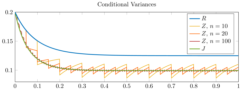
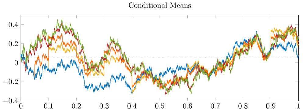
First, we illustrate our results from Section 3 in the setting with deterministic equidistant information dates tk=kΔnt_{k}=k\Delta_{n}, k=1,,nk=1,\dots,n, where Δn=Tn\Delta_{n}=\frac{T}{n}. Recall that the variance of the discrete-time expert in that case is

Γ(n)=1ΔnσJ2\Gamma^{(n)}=\frac{1}{\Delta_{n}}\sigma_{J}^{2}

and that expert opinions are defined as in (3.2) by

Zk(n)=μtk+1ΔnσJtktk+1dWsJZ^{(n)}_{k}=\mu_{t_{k}}+\frac{1}{\Delta_{n}}\sigma_{J}\int_{t_{k}}^{t_{k+1}}\mathrm{d}W^{J}_{s}

for k=1,,nk=1,\dots,n. In Figure 6.1 we plot the filters of the RR-, JJ- and ZZ-investor against time. For the ZZ-investor we consider the cases n=10,20,100n=10,20,100. In the upper plot one sees the conditional variances QRQ^{R} and QJQ^{J} as well as QZ,nQ^{Z,n} plotted against time. The lower plot shows a realization of the conditional means mRm^{R}, mJm^{J} and mZ,nm^{Z,n} for the same parameters.

Recall that QRQ^{R} and QJQ^{J} as well as QZ,nQ^{Z,n} for any nn\in\mathbb{N} are deterministic. In the upper plot of Figure 6.1 one sees that for any fixed t[0,T]t\in[0,T], the value of QtJQ^{J}_{t} as well as the value of QtZ,nQ^{Z,n}_{t} for any nn is less or equal than the value of QtRQ^{R}_{t}. This is due to Lemma 2.4. For the ZZ-investors one sees that the updates at information dates lead to a decrease in the conditional variance. As the number nn increases, the conditional variances QtZ,nQ^{Z,n}_{t} approach QtJQ^{J}_{t} for any t[0,T]t\in[0,T]. This is due to what has been shown in Theorem 3.2.

Note that for tt going to infinity, QtRQ^{R}_{t} and QtJQ^{J}_{t} approach a finite value. Convergence has been proven in Proposition 4.6 of Gabih et al. [11] for markets with d=1d=1 stock and generalized in Theorem 4.1 of Sass et al. [23] for markets with an arbitrary number of stocks. For (QtZ,n)t0(Q^{Z,n}_{t})_{t\geq 0} we observe a periodic behavior with asymptotic upper and lower bounds in the limit. This has been studied in detail in Sass et al. [23, Sec. 4.2].

In the lower subplot we show a realization of the various conditional means. For mZ,nm^{Z,n} the updating steps at information dates are visible. In general, we observe that when increasing the value of nn, the distance between the paths of mJm^{J} and mZ,nm^{Z,n} becomes smaller, as shown in Theorem 3.3.

Refer to caption
Refer to caption
Figure 6.1: A simulation of the filters for deterministic equidistant information dates. The upper subplot shows the conditional variances of the RR-, JJ- and ZZ-investor for various values of nn, the lower subplot shows a realization of the corresponding conditional means. The dashed black line is the mean reversion level δ\delta of the drift.

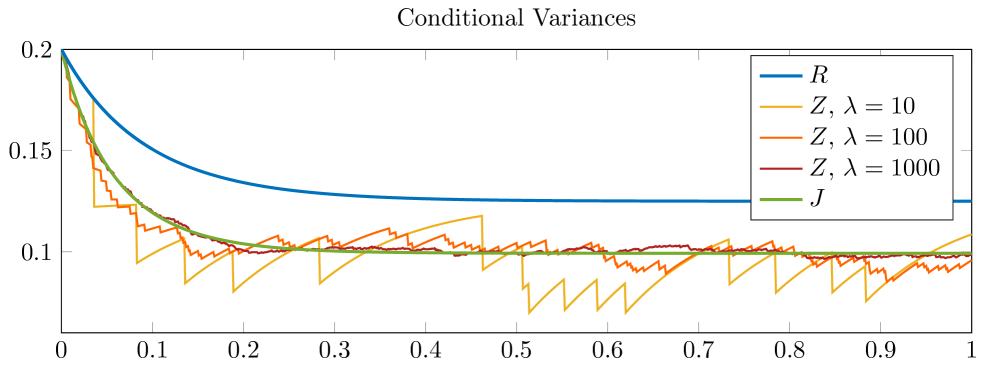
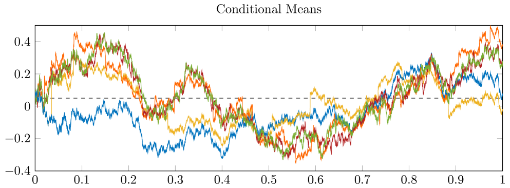
The analogous simulation can be done for the setting of Section 4 with random information dates TkT_{k} defined as the jump times of a Poisson process. We again suppose that the model parameters are as given in Table 6.1. Recall that under Assumption 4.1 the expert’s variance is of the form Γ(λ)=λσJ2\Gamma^{(\lambda)}=\lambda\sigma_{J}^{2} with expert opinions given as in (4.2) via

Zk(λ)=μTk+λσJk1λkλdWsJ.Z_{k}^{(\lambda)}=\mu_{T_{k}}+\lambda\sigma_{J}\int_{\frac{k-1}{\lambda}}^{\frac{k}{\lambda}}\mathrm{d}W^{J}_{s}.

Figure 6.2 shows, in addition to the filters of the RR- and JJ-investor, the filters of the ZZ-investor for different intensities λ\lambda. Note that the conditional variances of the filter in the case of the ZZ-investor behave qualitatively like in the situation with deterministic information dates. The time at which the expert opinions arrive is now random, however. The waiting times between two information dates are exponentially distributed with parameter λ\lambda. As a consequence, the updates for the ZZ-investor do not take place as regularly as in Figure 6.1.

The upper plot of Figure 6.2 shows realizations for λ=10,100,1000\lambda=10,100,1000. In general, by increasing the value of the parameter λ\lambda, one can increase the frequency of information dates, causing convergence of QtZ,λQ^{Z,\lambda}_{t} to QtJQ^{J}_{t} for any t[0,T]t\in[0,T], as shown in Theorem 4.6. In the lower subplot, we see the corresponding realizations of mZ,λm^{Z,\lambda}, in addition to mRm^{R} and mJm^{J} as before. Again, the updates in the conditional mean of the ZZ-investor are visible. What is also striking is that, when we consider the ZZ-investor with intensity λ=10\lambda=10, there are times where the distance between two sequent information dates is rather big. During those times, the conditional mean of the ZZ-investor comes closer to the conditional mean of the RR-investor who does not observe any expert opinion. When the intensity λ\lambda is increased, however, the conditional mean of the ZZ-investor approaches the conditional mean of the JJ-investor. For λ=1000\lambda=1000, the conditional means mZ,λm^{Z,\lambda} and mJm^{J} already behave quite similarly. Note, however, that for fixed information dates mZ,nm^{Z,n} is rather close to mJm^{J} for n=100n=100 already. Convergence of mZ,λm^{Z,\lambda} to mJm^{J} has been shown in Theorem 4.7. The difference in the speed of convergence when comparing the situation with equidistant information dates to the situation with random information dates is also discussed there.

Refer to caption
Refer to caption
Figure 6.2: A simulation of the filters for random information dates coming as jump times of a Poisson process. The upper subplot shows the conditional variances of the RR- and JJ-investor as well as realizations of QZ,λQ^{Z,\lambda} for various intensities λ\lambda, the lower subplot shows a realization of the corresponding conditional means. The dashed black line is the mean reversion level δ\delta of the drift.

In the remaining part of this section we want to illustrate the convergence results in the portfolio optimization problem that was introduced in Section 5. Recall that the value function of the HH-investor has the form

VH(x0)=log(x0)+120Ttr((σRσR)1(Σt+mtmt𝔼[QtH]))dt,V^{H}(x_{0})=\log(x_{0})+\frac{1}{2}\int_{0}^{T}\operatorname{tr}\bigl{(}(\sigma_{R}\sigma_{R}^{\top})^{-1}\bigl{(}\Sigma_{t}+m_{t}m_{t}^{\top}-\operatorname{\mathbb{E}}[Q^{H}_{t}]\bigr{)}\bigr{)}\,\mathrm{d}t, (6.1)

i.e. it is an integral functional of the conditional covariance matrices (QtH)t[0,T](Q^{H}_{t})_{t\in[0,T]}. This leads to convergence of VZ,nV^{Z,n} and VZ,λV^{Z,\lambda} to VJV^{J} when nn, respectively λ\lambda, goes to infinity, see Corollaries 5.2 and 5.3. In Table 2(a) we list the value functions of the RR-investor and of the JJ-investor as well as the value function of the ZZ-investor in the setting with nn equidistant information dates for different values of nn. We assume that investors have initial capital x0=1x_{0}=1 and that the model parameters are again those from Table 6.1. We see that the value functions VZ,n(1)V^{Z,n}(1) are increasing in nn and approach the value VJ(1)V^{J}(1) for large values of nn.

Calculating the value function of the ZZ-investor in the situation with non-deterministic information dates is a little more involved. This is because the conditional covariance matrices (QtZ,λ)t[0,T](Q^{Z,\lambda}_{t})_{t\in[0,T]} are then also non-deterministic. The value function, see again (6.1), depends on the expectation of QtZ,λQ^{Z,\lambda}_{t} for t[0,T]t\in[0,T]. This value cannot be calculated easily. To determine the value function numerically for the parameters in Table 6.1, we therefore perform for each value of λ\lambda a Monte Carlo simulation with 10 00010\,000 iterations. In each iteration, we generate a sequence of information dates as jump times of a Poisson process with intensity λ\lambda and calculate the corresponding conditional variances (QtZ,λ)t[0,T](Q^{Z,\lambda}_{t})_{t\in[0,T]}. By taking an average of all simulations this leads to a good approximation of VZ,λ(1)V^{Z,\lambda}(1). The diffusion approximation VJ(1)V^{J}(1) is available in closed form, its computation does not require numerical methods. Table 2(b) shows the resulting estimations for VZ,λ(1)V^{Z,\lambda}(1) and in brackets the corresponding 95% confidence intervals.

The values VZ,λ(1)V^{Z,\lambda}(1) lie between VR(1)V^{R}(1) and VJ(1)V^{J}(1), they are increasing in the intensity λ\lambda and for large values of λ\lambda they approach the value VJ(1)V^{J}(1). This is in line with Corollary 5.3. We also observe that VZ,λ(1)VZ,n(1)V^{Z,\lambda}(1)\leq V^{Z,n}(1) when setting the intensity λ\lambda equal to the deterministic number nn. Recall that an intensity λ=n\lambda=n means that there are on average nn information dates in the time interval [0,1][0,1]. The randomness coming from the Poisson process however leads to a lower value function, compared to VZ,n(1)V^{Z,n}(1). This difference is negligible for large intensities.

HH nn VH,n(1)V^{H,n}(1)
RR 0.3410
ZZ 1010 0.5245
ZZ 100100 0.5511
ZZ 10001000 0.5531
ZZ 10 00010\,000 0.5533
JJ 0.5533
(a) Equidistant information dates
HH λ\lambda VH,λ(1)V^{H,\lambda}(1)
RR 0.3410
ZZ 1010 0.5221 (0.5211, 0.5230)
ZZ 100100 0.5499 (0.5496, 0.5502)
ZZ 10001000 0.5530 (0.5529, 0.5531)
ZZ 10 00010\,000 0.5533 (0.5533, 0.5533)
JJ 0.5533
(b) Random information dates
Table 6.2: Value function for different investors and in the situation with random information dates in brackets the 95% confidence intervals for the ZZ-investor

Appendix A Auxiliary Results

In this appendix we give the proof of Proposition 4.5 and collect some auxiliary results that are used in the proofs of our main results.

Proof of Proposition 4.5.

From Lemma 2.2 one directly obtains

ddtQtJ=L(QtJ)QtJ(σJσJ)1QtJ,\frac{\mathrm{d}}{\mathrm{d}t}Q^{J}_{t}=L(Q^{J}_{t})-Q^{J}_{t}(\sigma_{J}\sigma_{J}^{\top})^{-1}Q^{J}_{t},

and the representation of QtJQ^{J}_{t} follows immediately. From Lemma 2.3 recall that between information dates the matrix differential equation for QZ,λQ^{Z,\lambda} reads

ddtQtZ,λ=L(QtZ,λ).\frac{\mathrm{d}}{\mathrm{d}t}Q^{Z,\lambda}_{t}=L(Q^{Z,\lambda}_{t}).

Now we can use Proposition 4.4 to include the updates of QZ,λQ^{Z,\lambda} at information dates and write

dQtZ,λ=L(QtZ,λ)dt+d(ρ(λ)(QtZ,λ)Id)QtZ,λN(dt,du)\mathrm{d}Q^{Z,\lambda}_{t}=L(Q^{Z,\lambda}_{t})\,\mathrm{d}t+\int_{\mathbb{R}^{d}}\bigl{(}\rho^{(\lambda)}(Q^{Z,\lambda}_{t-})-I_{d}\bigr{)}Q^{Z,\lambda}_{t-}\,N(\mathrm{d}t,\mathrm{d}u) (A.1)

for ρ(λ)(Q)=Γ(λ)(Q+Γ(λ))1\rho^{(\lambda)}(Q)=\Gamma^{(\lambda)}(Q+\Gamma^{(\lambda)})^{-1}. Note that the integrand is matrix-valued and the integral is defined componentwise. By (A.1) we can write

QtZ,λ\displaystyle Q^{Z,\lambda}_{t} =Σ0+0tL(QsZ,λ)ds+0td(ρ(λ)(QsZ,λ)Id)QsZ,λN(ds,du)\displaystyle=\Sigma_{0}+\int_{0}^{t}L(Q^{Z,\lambda}_{s})\,\mathrm{d}s+\int_{0}^{t}\int_{\mathbb{R}^{d}}\bigl{(}\rho^{(\lambda)}(Q^{Z,\lambda}_{s-})-I_{d}\bigr{)}Q^{Z,\lambda}_{s-}\,N(\mathrm{d}s,\mathrm{d}u) (A.2)
=Σ0+0tL(QsZ,λ)ds+0td(ρ(λ)(QsZ,λ)Id)QsZ,λN~(ds,du)\displaystyle=\Sigma_{0}+\int_{0}^{t}L(Q^{Z,\lambda}_{s})\,\mathrm{d}s+\int_{0}^{t}\int_{\mathbb{R}^{d}}\bigl{(}\rho^{(\lambda)}(Q^{Z,\lambda}_{s-})-I_{d}\bigr{)}Q^{Z,\lambda}_{s-}\,\tilde{N}(\mathrm{d}s,\mathrm{d}u)
+0td(ρ(λ)(QsZ,λ)Id)QsZ,λν(ds,du).\displaystyle\quad+\int_{0}^{t}\int_{\mathbb{R}^{d}}\bigl{(}\rho^{(\lambda)}(Q^{Z,\lambda}_{s-})-I_{d}\bigr{)}Q^{Z,\lambda}_{s-}\,\nu(\mathrm{d}s,\mathrm{d}u).

We see that

(ρ(λ)(Q)Id)Q=(Γ(λ)(Q+Γ(λ))1Id)Q=Q(Q+Γ(λ))1Q=Q(Q+λσJσJ)1Q.\bigl{(}\rho^{(\lambda)}(Q)-I_{d}\bigr{)}Q=\bigl{(}\Gamma^{(\lambda)}(Q+\Gamma^{(\lambda)})^{-1}-I_{d}\bigr{)}Q=-Q(Q+\Gamma^{(\lambda)})^{-1}Q=-Q(Q+\lambda\sigma_{J}\sigma_{J}^{\top})^{-1}Q.

Therefore, the last integral in (A.2) can be written as

0td(ρ(λ)(QsZ,λ)Id)QsZ,λν(ds,du)\displaystyle\int_{0}^{t}\int_{\mathbb{R}^{d}}\bigl{(}\rho^{(\lambda)}(Q^{Z,\lambda}_{s-})-I_{d}\bigr{)}Q^{Z,\lambda}_{s-}\,\nu(\mathrm{d}s,\mathrm{d}u) =0tdQsZ,λ(QsZ,λ+λσJσJ)1QsZ,λν(ds,du)\displaystyle=-\int_{0}^{t}\int_{\mathbb{R}^{d}}Q^{Z,\lambda}_{s-}(Q^{Z,\lambda}_{s-}+\lambda\sigma_{J}\sigma_{J}^{\top})^{-1}Q^{Z,\lambda}_{s-}\,\nu(\mathrm{d}s,\mathrm{d}u)
=0tdQsZ,λ(QsZ,λ+λσJσJ)1QsZ,λφ(u)λduds\displaystyle=-\int_{0}^{t}\int_{\mathbb{R}^{d}}Q^{Z,\lambda}_{s-}(Q^{Z,\lambda}_{s-}+\lambda\sigma_{J}\sigma_{J}^{\top})^{-1}Q^{Z,\lambda}_{s-}\varphi(u)\lambda\,\mathrm{d}u\,\mathrm{d}s
=0tλQsZ,λ(QsZ,λ+λσJσJ)1QsZ,λds,\displaystyle=-\int_{0}^{t}\lambda Q^{Z,\lambda}_{s-}(Q^{Z,\lambda}_{s-}+\lambda\sigma_{J}\sigma_{J}^{\top})^{-1}Q^{Z,\lambda}_{s-}\,\mathrm{d}s,

where the second equality follows from Proposition 4.4 and the last equality is due to φ\varphi being a probability density. Plugging back in into (A.2) yields

QtZ,λ\displaystyle Q^{Z,\lambda}_{t} =Σ0+0t(L(QsZ,λ)λQsZ,λ(QsZ,λ+λσJσJ)1QsZ,λ)ds\displaystyle=\Sigma_{0}+\int_{0}^{t}\bigl{(}L(Q^{Z,\lambda}_{s})-\lambda Q^{Z,\lambda}_{s-}(Q^{Z,\lambda}_{s-}+\lambda\sigma_{J}\sigma_{J}^{\top})^{-1}Q^{Z,\lambda}_{s-}\bigr{)}\,\mathrm{d}s
0tdQsZ,λ(QsZ,λ+λσJσJ)1QsZ,λN~(ds,du),\displaystyle\quad-\int_{0}^{t}\int_{\mathbb{R}^{d}}Q^{Z,\lambda}_{s-}(Q^{Z,\lambda}_{s-}+\lambda\sigma_{J}\sigma_{J}^{\top})^{-1}Q^{Z,\lambda}_{s-}\,\tilde{N}(\mathrm{d}s,\mathrm{d}u),

and the representation of QtZ,λQ^{Z,\lambda}_{t} is also proven. ∎

The following lemma can be interpreted as a discrete version of Gronwall’s Lemma for error accumulation. A statement similar to Lemma A.1 can be found in Demailly [8, Sec. 8.2.4].

Lemma A.1.

Let (aj)j=0,,n(a_{j})_{j=0,\dots,n}, (hj)j=0,,n(h_{j})_{j=0,\dots,n} be real-valued sequences with aj0a_{j}\geq 0, hj>0h_{j}>0, and L>0L>0, b0b\geq 0 real numbers such that

aj+1(1+hjL)aj+hjb,j=0,1,,n1.a_{j+1}\leq(1+h_{j}L)a_{j}+h_{j}b,\qquad j=0,1,\dots,n-1.

Then for all j=0,1,,nj=0,1,\dots,n it holds

ajeLtj1Lb+eLtja0,a_{j}\leq\frac{\mathrm{e}^{Lt_{j}}-1}{L}b+\mathrm{e}^{Lt_{j}}a_{0},

where tj=i=0j1hi.t_{j}=\sum_{i=0}^{j-1}h_{i}.

Proof.

The proof can be done by induction. For j=0j=0 the claim is obvious. For the induction step we observe that 1+xex1+x\leq\mathrm{e}^{x} for all xx\in\mathbb{R} and hence

aj+1(1+hjL)aj+hjbehjLaj+hjb.a_{j+1}\leq(1+h_{j}L)a_{j}+h_{j}b\leq\mathrm{e}^{h_{j}L}a_{j}+h_{j}b.

Due to the induction hypothesis we therefore have

aj+1\displaystyle a_{j+1} ehjL(eLtj1Lb+eLtja0)+hjb\displaystyle\leq\mathrm{e}^{h_{j}L}\Bigl{(}\frac{\mathrm{e}^{Lt_{j}}-1}{L}b+\mathrm{e}^{Lt_{j}}a_{0}\Bigr{)}+h_{j}b
=(eL(tj+hj)eLhj+hjLL)b+eL(tj+hj)a0\displaystyle=\Bigl{(}\frac{\mathrm{e}^{L(t_{j}+h_{j})}-\mathrm{e}^{Lh_{j}}+h_{j}L}{L}\Bigr{)}b+\mathrm{e}^{L(t_{j}+h_{j})}a_{0}
eLtj+11Lb+eLtj+1a0,\displaystyle\leq\frac{\mathrm{e}^{Lt_{j+1}}-1}{L}b+\mathrm{e}^{Lt_{j+1}}a_{0},

which completes the proof. ∎

The next lemmas are used in the proof of Theorem 3.3. Firstly, the following lemma is a Cauchy–Schwarz inequality for multidimensional integrals.

Lemma A.2.

Let (Xs)s[0,t](X_{s})_{s\in[0,t]} be an d\mathbb{R}^{d}-valued stochastic process. Then

𝔼[0tXsds2]t0t𝔼[Xs2]ds.\operatorname{\mathbb{E}}\biggl{[}\biggl{\lVert}\int_{0}^{t}X_{s}\,\mathrm{d}s\biggr{\rVert}^{2}\biggr{]}\leq t\int_{0}^{t}\operatorname{\mathbb{E}}\bigl{[}\lVert X_{s}\rVert^{2}\bigr{]}\,\mathrm{d}s.
Proof.

Firstly, pulling the norm into the integral increases the expression on the left-hand side, so

𝔼[0tXsds2]𝔼[(0tXsds)2].\operatorname{\mathbb{E}}\biggl{[}\biggl{\lVert}\int_{0}^{t}X_{s}\,\mathrm{d}s\biggr{\rVert}^{2}\biggr{]}\leq\operatorname{\mathbb{E}}\biggl{[}\biggl{(}\int_{0}^{t}\lVert X_{s}\rVert\,\mathrm{d}s\biggr{)}^{2}\biggr{]}.

Now we can apply the usual Cauchy–Schwarz inequality to the one-dimensional integral and get

𝔼[(0tXsds)2]𝔼[t0tXs2ds]=t0t𝔼[Xs2]ds.\operatorname{\mathbb{E}}\biggl{[}\biggl{(}\int_{0}^{t}\lVert X_{s}\rVert\,\mathrm{d}s\biggr{)}^{2}\biggr{]}\leq\operatorname{\mathbb{E}}\biggl{[}t\int_{0}^{t}\lVert X_{s}\rVert^{2}\,\mathrm{d}s\biggr{]}=t\int_{0}^{t}\operatorname{\mathbb{E}}\bigl{[}\lVert X_{s}\rVert^{2}\bigr{]}\,\mathrm{d}s.

The last step is due to Fubini. ∎

A key tool for estimations involving stochastic integrals is the Itô isometry. The following lemma uses the isometry to obtain an estimation for multivariate integrals.

Lemma A.3.

Let W=(Ws)s[0,t]W=(W_{s})_{s\in[0,t]} be an mm-dimensional Brownian motion. Let (Hs)s[0,t](H_{s})_{s\in[0,t]} be an d×m\mathbb{R}^{d\times m}-valued stochastic process that is independent of WW, and τ\tau a stopping time that is bounded by tt and also independent of WW. Then

𝔼[0τHsdWs2]=𝔼[0τHsF2ds]Cnorm𝔼[0τHs2ds],\operatorname{\mathbb{E}}\biggl{[}\biggl{\lVert}\int_{0}^{\tau}H_{s}\,\mathrm{d}W_{s}\biggr{\rVert}^{2}\biggr{]}=\operatorname{\mathbb{E}}\biggl{[}\int_{0}^{\tau}\lVert H_{s}\rVert_{F}^{2}\,\mathrm{d}s\biggr{]}\leq C_{\textrm{norm}}\operatorname{\mathbb{E}}\biggl{[}\int_{0}^{\tau}\lVert H_{s}\rVert^{2}\,\mathrm{d}s\biggr{]},

where F\lVert\cdot\rVert_{F} denotes the Frobenius norm and Cnorm>0C_{\textrm{norm}}>0 only depends on the dimension d×md\times m of the integrand HH.

Proof.

Note that for fixed, deterministic tt, the integral 0tHsdWs\int_{0}^{t}H_{s}\,\mathrm{d}W_{s} is a random variable with values in d\mathbb{R}^{d}. The ii-th entry is

j=1m0tHsijdWsj.\sum_{j=1}^{m}\int_{0}^{t}H^{ij}_{s}\,\mathrm{d}W^{j}_{s}.

Hence,

0tHsdWs2=i=1d(j=1m0tHsijdWsj)2.\biggl{\lVert}\int_{0}^{t}H_{s}\,\mathrm{d}W_{s}\biggr{\rVert}^{2}=\sum_{i=1}^{d}\biggl{(}\sum_{j=1}^{m}\int_{0}^{t}H^{ij}_{s}\,\mathrm{d}W^{j}_{s}\biggr{)}^{2}.

When applying the expectation, we get due to independence

𝔼[0tHsdWs2]\displaystyle\operatorname{\mathbb{E}}\biggl{[}\biggl{\lVert}\int_{0}^{t}H_{s}\,\mathrm{d}W_{s}\biggr{\rVert}^{2}\biggr{]} =i=1dj,k=1m𝔼[0tHsijdWsj0tHsikdWsk]\displaystyle=\sum_{i=1}^{d}\sum_{j,k=1}^{m}\operatorname{\mathbb{E}}\biggl{[}\int_{0}^{t}H^{ij}_{s}\,\mathrm{d}W^{j}_{s}\int_{0}^{t}H^{ik}_{s}\,\mathrm{d}W^{k}_{s}\biggr{]} (A.3)
=i=1dj=1m𝔼[(0tHsijdWsj)2].\displaystyle=\sum_{i=1}^{d}\sum_{j=1}^{m}\operatorname{\mathbb{E}}\biggl{[}\biggl{(}\int_{0}^{t}H^{ij}_{s}\,\mathrm{d}W^{j}_{s}\biggr{)}^{2}\biggr{]}.

Note that we can consider the filtration (𝒢s)s[0,t](\mathcal{G}_{s})_{s\in[0,t]} where 𝒢s=σ(Wu,us)σ(Hu,u[0,t])\mathcal{G}_{s}=\sigma(W_{u},u\leq s)\vee\sigma(H_{u},u\in[0,t]). Since HH and WW are independent, WW is a Brownian motion with respect to (𝒢s)s[0,t](\mathcal{G}_{s})_{s\in[0,t]}. Also, HH is obviously adapted with respect to (𝒢s)s[0,t](\mathcal{G}_{s})_{s\in[0,t]}. Hence, we can apply the usual Itô isometry and obtain that the right-hand side of (A.3) equals

i=1dj=1m𝔼[0t(Hsij)2ds]=𝔼[0tHsF2ds].\sum_{i=1}^{d}\sum_{j=1}^{m}\operatorname{\mathbb{E}}\biggl{[}\int_{0}^{t}(H^{ij}_{s})^{2}\,\mathrm{d}s\biggr{]}=\operatorname{\mathbb{E}}\biggl{[}\int_{0}^{t}\lVert H_{s}\rVert_{F}^{2}\,\mathrm{d}s\biggr{]}.

Now when taking into account the stopping time τ\tau, we can write

𝔼[0τHsdWs2]=𝔼[0t𝟙{sτ}HsdWs2].\operatorname{\mathbb{E}}\biggl{[}\biggl{\lVert}\int_{0}^{\tau}H_{s}\,\mathrm{d}W_{s}\biggr{\rVert}^{2}\biggr{]}=\operatorname{\mathbb{E}}\biggl{[}\biggl{\lVert}\int_{0}^{t}\mathbbm{1}_{\{s\leq\tau\}}H_{s}\,\mathrm{d}W_{s}\biggr{\rVert}^{2}\biggr{]}.

Since τ\tau is independent of WW we can deduce from the previous part of the proof that

𝔼[0t𝟙{sτ}HsdWs2]=𝔼[0t𝟙{sτ}HsF2ds]=𝔼[0τHsF2ds].\operatorname{\mathbb{E}}\biggl{[}\biggl{\lVert}\int_{0}^{t}\mathbbm{1}_{\{s\leq\tau\}}H_{s}\,\mathrm{d}W_{s}\biggr{\rVert}^{2}\biggr{]}=\operatorname{\mathbb{E}}\biggl{[}\int_{0}^{t}\lVert\mathbbm{1}_{\{s\leq\tau\}}H_{s}\rVert_{F}^{2}\,\mathrm{d}s\biggr{]}=\operatorname{\mathbb{E}}\biggl{[}\int_{0}^{\tau}\lVert H_{s}\rVert_{F}^{2}\,\mathrm{d}s\biggr{]}.

Equivalence of norms implies the existence of the constant Cnorm>0C_{\textrm{norm}}>0 with the property that

𝔼[0τHsF2ds]Cnorm𝔼[0τHs2ds],\operatorname{\mathbb{E}}\biggl{[}\int_{0}^{\tau}\lVert H_{s}\rVert_{F}^{2}\,\mathrm{d}s\biggr{]}\leq C_{\textrm{norm}}\operatorname{\mathbb{E}}\biggl{[}\int_{0}^{\tau}\lVert H_{s}\rVert^{2}\,\mathrm{d}s\biggr{]},

which concludes the proof. ∎

Another estimate that is useful in the convergence proofs is given in the following lemma.

Lemma A.4.

Let κ>0\kappa>0 and let QκQ^{\kappa} be a symmetric and positive-definite matrix in d×d\mathbb{R}^{d\times d} with QκCQ\lVert Q^{\kappa}\rVert\leq C_{Q} for all κ\kappa. Then there exists a constant C¯>0\bar{C}>0 such that

QκQκ(Qκ+κσJσJ)1κσJσJC¯κ.\Bigl{\lVert}Q^{\kappa}-Q^{\kappa}\bigl{(}Q^{\kappa}+\kappa\sigma_{J}\sigma_{J}^{\top}\bigr{)}^{-1}\kappa\sigma_{J}\sigma_{J}^{\top}\Bigr{\rVert}\leq\frac{\bar{C}}{\kappa}.
Proof.

For abbreviation let A:=QκA:=Q^{\kappa}, B:=σJσJB:=\sigma_{J}\sigma_{J}^{\top}. Then we can write

AA(A+κB)1κB\displaystyle A-A(A+\kappa B)^{-1}\kappa B =A(A+κB)1(A+κBκB)=A(A+κB)1A\displaystyle=A(A+\kappa B)^{-1}(A+\kappa B-\kappa B)=A(A+\kappa B)^{-1}A
=(A1(A+κB)A1)1=(A1+κA1BA1)1,\displaystyle=\bigl{(}A^{-1}(A+\kappa B)A^{-1}\bigr{)}^{-1}=\bigl{(}A^{-1}+\kappa A^{-1}BA^{-1}\bigr{)}^{-1},

and therefore

AA(A+κB)1κB\displaystyle\bigl{\lVert}A-A(A+\kappa B)^{-1}\kappa B\bigr{\rVert} =(A1+κA1BA1)1=(λmin(A1+κA1BA1))1\displaystyle=\bigl{\lVert}\bigl{(}A^{-1}+\kappa A^{-1}BA^{-1}\bigr{)}^{-1}\bigr{\rVert}=\Bigl{(}\operatorname{\lambda_{\min}}(A^{-1}+\kappa A^{-1}BA^{-1})\Bigr{)}^{-1}
(λmin(A1)+λmin(κA1BA1))1(λmin(κA1BA1))1\displaystyle\leq\Bigl{(}\operatorname{\lambda_{\min}}(A^{-1})+\operatorname{\lambda_{\min}}(\kappa A^{-1}BA^{-1})\Bigr{)}^{-1}\leq\Bigl{(}\operatorname{\lambda_{\min}}(\kappa A^{-1}BA^{-1})\Bigr{)}^{-1}
=1κAB1A.\displaystyle=\frac{1}{\kappa}\lVert AB^{-1}A\rVert.

Hence, we obtain

QκQκ(Qκ+κσJσJ)1κσJσJCQ2(σJσJ)1κ=C¯κ,\Bigl{\lVert}Q^{\kappa}-Q^{\kappa}\bigl{(}Q^{\kappa}+\kappa\sigma_{J}\sigma_{J}^{\top}\bigr{)}^{-1}\kappa\sigma_{J}\sigma_{J}^{\top}\Bigr{\rVert}\leq\frac{C_{Q}^{2}\lVert(\sigma_{J}\sigma_{J}^{\top})^{-1}\rVert}{\kappa}=\frac{\bar{C}}{\kappa},

where C¯=CQ2(σJσJ)1\bar{C}=C_{Q}^{2}\lVert(\sigma_{J}\sigma_{J}^{\top})^{-1}\rVert. ∎

The next lemma states Gronwall’s Lemma in integral form which we use in the proofs of Theorems 4.6 and 4.7. A proof can be found for example in Pachpatte [20, Sec. 1.3].

Lemma A.5 (Gronwall).

Let I=[a,b]I=[a,b] be an interval and let u,αu,\alpha and β:I[0,)\beta\colon I\to[0,\infty) be continuous functions with

u(t)α(t)+atβ(s)u(s)dsu(t)\leq\alpha(t)+\int_{a}^{t}\beta(s)u(s)\,\mathrm{d}s

for all tIt\in I. Then

u(t)α(t)+atα(s)β(s)estβ(r)drdsu(t)\leq\alpha(t)+\int_{a}^{t}\alpha(s)\beta(s)\mathrm{e}^{\int_{s}^{t}\beta(r)\,\mathrm{d}r}\,\mathrm{d}s

for all tIt\in I.

In Section 4 we work with a Poisson random measure. An important property of the compensated Poisson measure that we use for the proof of Theorem 4.6 is given in the following lemma, see Proposition 2.16 in Cont and Tankov [5].

Lemma A.6.

For an integrable real-valued function f:[0,T]×df\colon[0,T]\times\mathbb{R}^{d}\to\mathbb{R}, the process (Xt)t0(X_{t})_{t\geq 0} with

Xt=0tdf(s,u)N~(ds,du)X_{t}=\int_{0}^{t}\int_{\mathbb{R}^{d}}f(s,u)\,\tilde{N}(\mathrm{d}s,\mathrm{d}u)

is a martingale with 𝔼[Xt]=0\operatorname{\mathbb{E}}[X_{t}]=0 and

var(Xt)=𝔼[Xt2]=𝔼[0tdf2(s,u)λφ(u)duds].\operatorname{var}(X_{t})=\operatorname{\mathbb{E}}[X_{t}^{2}]=\operatorname{\mathbb{E}}\biggl{[}\int_{0}^{t}\int_{\mathbb{R}^{d}}f^{2}(s,u)\lambda\varphi(u)\,\mathrm{d}u\,\mathrm{d}s\biggr{]}. (A.4)

Appendix B Proofs for Deterministic Information Dates

B.1 Proof of Theorem 3.2: Convergence of Covariance Matrices

Throughout the proof, we omit the superscript nn at information dates tk(n)t_{k}^{(n)} for the sake of better readability, keeping the dependence on nn in mind. The proof is based on finding a recursive formula for the distance between QtkZ,nQ^{Z,n}_{t_{k}-} and QtkJQ^{J}_{t_{k}} where we make use of an Euler approximation of QJQ^{J}.

Euler scheme approximation of 𝑸𝑱\boldsymbol{Q^{J}}.

Recall the dynamics of QJQ^{J} from Lemma 2.2. To shorten notation, let G:d×dd×dG\colon\mathbb{R}^{d\times d}\to\mathbb{R}^{d\times d} with

G(Q)=αQQα+ββQ((σRσR)1+(σJσJ)1)QG(Q)=-\alpha Q-Q\alpha+\beta\beta^{\top}-Q\bigl{(}(\sigma_{R}\sigma_{R}^{\top})^{-1}+(\sigma_{J}\sigma_{J}^{\top})^{-1}\bigr{)}Q

denote the right-hand side of the differential equation (2.2). Then (2.2) reads as

ddtQtJ=G(QtJ).\frac{\mathrm{d}}{\mathrm{d}t}Q^{J}_{t}=G(Q^{J}_{t}).

The first step is to approximate QJQ^{J} by an Euler scheme. Therefore, define QJ,nQ^{J,n} by setting

QtJ,n:=QtkJ+G(QtkJ)(ttk)Q^{J,n}_{t}:=Q^{J}_{t_{k}}+G(Q^{J}_{t_{k}})(t-t_{k}) (B.1)

for all t[tk,tk+1)t\in[t_{k},t_{k+1}). From a Taylor expansion we get that

QtJ=QtkJ+G(QtkJ)(ttk)+ξt(ttk)2Q^{J}_{t}=Q^{J}_{t_{k}}+G(Q^{J}_{t_{k}})(t-t_{k})+\xi_{t}(t-t_{k})^{2}

where ξ\xi is a matrix-valued function involving the second derivative of QtJQ^{J}_{t}. Since QJQ^{J} and its derivatives are bounded on [0,T][0,T], see Lemma 2.4, the matrices ξt\xi_{t} are bounded, hence the local truncation error is proportional to Δn2\Delta_{n}^{2}. In other words, there exists some CEuler>0C_{\text{Euler}}>0 such that

QtJQtJ,nCEulerΔn2\bigl{\lVert}Q^{J}_{t}-Q^{J,n}_{t}\bigr{\rVert}\leq C_{\text{Euler}}\Delta_{n}^{2} (B.2)

for all t[0,T]t\in[0,T].

Estimation of the error in 𝑮\boldsymbol{G}.

Let CeC_{e}, CQ>0C_{Q}>0 and let εd×d\varepsilon\in\mathbb{R}^{d\times d} with εCe\lVert\varepsilon\rVert\leq C_{e}, Qd×dQ\in\mathbb{R}^{d\times d} with QCQ\lVert Q\rVert\leq C_{Q}. Then

G(Q+ε)\displaystyle G(Q+\varepsilon) =α(Q+ε)(Q+ε)α+ββ(Q+ε)((σRσR)1+(σJσJ)1)(Q+ε)\displaystyle=-\alpha(Q+\varepsilon)-(Q+\varepsilon)\alpha+\beta\beta^{\top}-(Q+\varepsilon)\bigl{(}(\sigma_{R}\sigma_{R}^{\top})^{-1}+(\sigma_{J}\sigma_{J}^{\top})^{-1}\bigr{)}(Q+\varepsilon)
=G(Q)ε(α+((σRσR)1+(σJσJ)1)(Q+ε))\displaystyle=G(Q)-\varepsilon\bigl{(}\alpha+\bigl{(}(\sigma_{R}\sigma_{R}^{\top})^{-1}+(\sigma_{J}\sigma_{J}^{\top})^{-1}\bigr{)}(Q+\varepsilon)\bigr{)}
(α+Q((σRσR)1+(σJσJ)1))ε.\displaystyle\quad-\bigl{(}\alpha+Q\bigl{(}(\sigma_{R}\sigma_{R}^{\top})^{-1}+(\sigma_{J}\sigma_{J}^{\top})^{-1}\bigr{)}\bigr{)}\varepsilon.

Hence,

G(Q+ε)G(Q)ε(2α+(σRσR)1+(σJσJ)1(2Q+ε)).\lVert G(Q+\varepsilon)-G(Q)\rVert\leq\lVert\varepsilon\rVert\bigl{(}2\lVert\alpha\rVert+\lVert(\sigma_{R}\sigma_{R}^{\top})^{-1}+(\sigma_{J}\sigma_{J}^{\top})^{-1}\rVert(2\lVert Q\rVert+\lVert\varepsilon\rVert)\bigr{)}.

This implies that there exists a constant CG>0C_{G}>0 such that for all ε\varepsilon, Qd×dQ\in\mathbb{R}^{d\times d} with εCe\lVert\varepsilon\rVert\leq C_{e} and QCQ\lVert Q\rVert\leq C_{Q} it holds

G(Q+ε)G(Q)CGε.\lVert G(Q+\varepsilon)-G(Q)\rVert\leq C_{G}\lVert\varepsilon\rVert. (B.3)

Dynamics of 𝑸𝒁,𝒏\boldsymbol{Q^{Z,n}}.

Next, we take a look at the dynamics of QZ,nQ^{Z,n}, i.e. of the covariance matrix corresponding to the investor who observes the stock returns and the opinions of the discrete expert. We know that at information dates tkt_{k}, k=1,,nk=1,\dots,n, we have the update formula

QtkZ,n=Γ(n)(QtkZ,n+Γ(n))1QtkZ,n.Q^{Z,n}_{t_{k}}=\Gamma^{(n)}\bigl{(}Q^{Z,n}_{t_{k}-}+\Gamma^{(n)}\bigr{)}^{-1}Q^{Z,n}_{t_{k}-}.

Observe that

Γ(n)(QtkZ,n+Γ(n))1=(Id+QtkZ,n(Γ(n))1)1=(Id+ΔnQtkZ,n(σJσJ)1)1\Gamma^{(n)}\bigl{(}Q^{Z,n}_{t_{k}-}+\Gamma^{(n)}\bigr{)}^{-1}=\bigl{(}I_{d}+Q^{Z,n}_{t_{k}-}(\Gamma^{(n)})^{-1}\bigr{)}^{-1}=\bigl{(}I_{d}+\Delta_{n}Q^{Z,n}_{t_{k}-}(\sigma_{J}\sigma_{J}^{\top})^{-1}\bigr{)}^{-1}

which can be written as the Neumann series

i=0(ΔnQtkZ,n(σJσJ)1)i=IdΔnQtkZ,n(σJσJ)1+i=2(ΔnQtkZ,n(σJσJ)1)i.\sum_{i=0}^{\infty}\bigl{(}-\Delta_{n}Q^{Z,n}_{t_{k}-}(\sigma_{J}\sigma_{J}^{\top})^{-1}\bigr{)}^{i}=I_{d}-\Delta_{n}Q^{Z,n}_{t_{k}-}(\sigma_{J}\sigma_{J}^{\top})^{-1}+\sum_{i=2}^{\infty}\bigl{(}-\Delta_{n}Q^{Z,n}_{t_{k}-}(\sigma_{J}\sigma_{J}^{\top})^{-1}\bigr{)}^{i}.

It follows that

QtkZ,n=QtkZ,nΔnQtkZ,n(σJσJ)1QtkZ,n+R¯nQ^{Z,n}_{t_{k}}=Q^{Z,n}_{t_{k}-}-\Delta_{n}Q^{Z,n}_{t_{k}-}(\sigma_{J}\sigma_{J}^{\top})^{-1}Q^{Z,n}_{t_{k}-}+\bar{R}^{n} (B.4)

where R¯nrΔn2\lVert\bar{R}^{n}\rVert\leq r\Delta_{n}^{2}, since QtkZ,nQ^{Z,n}_{t_{k}-} is bounded. Between information dates, the matrix QZ,nQ^{Z,n} follows the dynamics

ddtQtZ,n=αQtZ,nQtZ,nα+ββQtZ,n(σRσR)1QtZ,n\frac{\mathrm{d}}{\mathrm{d}t}Q^{Z,n}_{t}=-\alpha Q^{Z,n}_{t}-Q^{Z,n}_{t}\alpha+\beta\beta^{\top}-Q^{Z,n}_{t}(\sigma_{R}\sigma_{R}^{\top})^{-1}Q^{Z,n}_{t}

for t[tk,tk+1)t\in[t_{k},t_{k+1}).

One time step for 𝑸𝒁,𝒏\boldsymbol{Q^{Z,n}}.

In the following, we construct a formula that connects Qtk+1Z,nQ^{Z,n}_{t_{k+1}-} with QtkZ,nQ^{Z,n}_{t_{k}-}. Firstly, by making a Taylor expansion we see that

Qtk+1Z,n=QtkZ,n+(αQtkZ,nQtkZ,nα+ββQtkZ,n(σRσR)1QtkZ,n)Δn+Ln,Q^{Z,n}_{t_{k+1}-}=Q^{Z,n}_{t_{k}}+\bigl{(}-\alpha Q^{Z,n}_{t_{k}}-Q^{Z,n}_{t_{k}}\alpha+\beta\beta^{\top}-Q^{Z,n}_{t_{k}}(\sigma_{R}\sigma_{R}^{\top})^{-1}Q^{Z,n}_{t_{k}}\bigr{)}\Delta_{n}+L^{n},

where LnCLΔn2\lVert L^{n}\rVert\leq C_{L}\Delta_{n}^{2}. Now, when inserting the representation of QtkZ,nQ^{Z,n}_{t_{k}} from (B.4) and rearranging terms we can conclude that

Qtk+1Z,n=QtkZ,n+ΔnG(QtkZ,n)+Rn,Q^{Z,n}_{t_{k+1}-}=Q^{Z,n}_{t_{k}-}+\Delta_{n}G(Q^{Z,n}_{t_{k}-})+R^{n}, (B.5)

where RnR^{n} is a matrix with RnCTaylorΔn2\lVert R^{n}\rVert\leq C_{\text{Taylor}}\Delta_{n}^{2} for CTaylor>0C_{\text{Taylor}}>0.

Recursive formula for estimation error.

For k=0,,nk=0,\dots,n, define Ak=QtkZ,nQtkJA_{k}=Q^{Z,n}_{t_{k}-}-Q^{J}_{t_{k}} and ak=Aka_{k}=\lVert A_{k}\rVert. Our aim is to find a recursive formula that yields an upper bound for these estimation errors. Let k0k\geq 0. Then we have by (B.5) that

ak+1=Ak+1=Qtk+1Z,nQtk+1J=QtkZ,n+ΔnG(QtkZ,n)+RnQtk+1J.a_{k+1}=\lVert A_{k+1}\rVert=\lVert Q^{Z,n}_{t_{k+1}-}-Q^{J}_{t_{k+1}}\rVert=\lVert Q^{Z,n}_{t_{k}-}+\Delta_{n}G(Q^{Z,n}_{t_{k}-})+R^{n}-Q^{J}_{t_{k+1}}\rVert.

Thus, by definition of AkA_{k} and QJ,nQ^{J,n} as given in (B.1),

ak+1\displaystyle a_{k+1} =(QtkJ+Ak)+ΔnG(QtkJ+Ak)+RnQtk+1J\displaystyle=\lVert(Q^{J}_{t_{k}}+A_{k})+\Delta_{n}G(Q^{J}_{t_{k}}+A_{k})+R^{n}-Q^{J}_{t_{k+1}}\rVert
=QtkJ+Δn(G(QtkJ)+G(QtkJ+Ak)G(QtkJ))+Ak+RnQtk+1J\displaystyle=\lVert Q^{J}_{t_{k}}+\Delta_{n}\bigl{(}G(Q^{J}_{t_{k}})+G(Q^{J}_{t_{k}}+A_{k})-G(Q^{J}_{t_{k}})\bigr{)}+A_{k}+R^{n}-Q^{J}_{t_{k+1}}\rVert
=Qtk+1J,n+Δn(G(QtkJ+Ak)G(QtkJ))+Ak+RnQtk+1J.\displaystyle=\lVert Q^{J,n}_{t_{k+1}-}+\Delta_{n}\bigl{(}G(Q^{J}_{t_{k}}+A_{k})-G(Q^{J}_{t_{k}})\bigr{)}+A_{k}+R^{n}-Q^{J}_{t_{k+1}}\rVert.

Now, the estimations from (B.2), (B.3) and (B.5) yield

ak+1CEulerΔn2+ΔnCGAk+Ak+CTaylorΔn2=(1+ΔnCG)ak+(CEuler+CTaylor)Δn2.a_{k+1}\leq C_{\text{Euler}}\Delta_{n}^{2}+\Delta_{n}C_{G}\lVert A_{k}\rVert+\lVert A_{k}\rVert+C_{\text{Taylor}}\Delta_{n}^{2}=(1+\Delta_{n}C_{G})a_{k}+(C_{\text{Euler}}+C_{\text{Taylor}})\Delta_{n}^{2}.

By a discrete version of Gronwall’s Lemma, see Lemma A.1 in the appendix, this implies

akeCGkΔn1CG(CEuler+CTaylor)ΔneCGT1CG(CEuler+CTaylor)Δn=:C~Δn.a_{k}\leq\frac{\mathrm{e}^{C_{G}k\Delta_{n}}-1}{C_{G}}(C_{\text{Euler}}+C_{\text{Taylor}})\Delta_{n}\leq\frac{\mathrm{e}^{C_{G}T}-1}{C_{G}}(C_{\text{Euler}}+C_{\text{Taylor}})\Delta_{n}=:\tilde{C}\Delta_{n}.

Therefore, for all k=0,,nk=0,\dots,n we have

QtkZ,nQtkJC~Δn.\lVert Q^{Z,n}_{t_{k}-}-Q^{J}_{t_{k}}\rVert\leq\tilde{C}\Delta_{n}. (B.6)

Difference of 𝑸𝒕𝒁,𝒏\boldsymbol{Q^{Z,n}_{t}} and 𝑸𝒕𝑱\boldsymbol{Q^{J}_{t}} for arbitrary 𝒕\boldsymbol{t}.

We now show that there exists some KQ>0K_{Q}>0 such that QtZ,nQtJKQΔn\lVert Q^{Z,n}_{t}-Q^{J}_{t}\rVert\leq K_{Q}\Delta_{n} for all t[0,T]t\in[0,T]. Let t[0,T]t\in[0,T] with t[tk,tk+1)t\in[t_{k},t_{k+1}). We can write

QtZ,nQtJ=(QtZ,nQtkZ,n)+(QtkZ,nQtkJ)+(QtkJQtJ),Q^{Z,n}_{t}-Q^{J}_{t}=(Q^{Z,n}_{t}-Q^{Z,n}_{t_{k}-})+(Q^{Z,n}_{t_{k}-}-Q^{J}_{t_{k}})+(Q^{J}_{t_{k}}-Q^{J}_{t}),

and hence

QtZ,nQtJQtZ,nQtkZ,n+QtkZ,nQtkJ+QtkJQtJ.\lVert Q^{Z,n}_{t}-Q^{J}_{t}\rVert\leq\lVert Q^{Z,n}_{t}-Q^{Z,n}_{t_{k}-}\rVert+\lVert Q^{Z,n}_{t_{k}-}-Q^{J}_{t_{k}}\rVert+\lVert Q^{J}_{t_{k}}-Q^{J}_{t}\rVert.

By (B.6), the second summand is bounded by C~Δn\tilde{C}\Delta_{n}. We now take a look at the other two summands. By definition of QJ,nQ^{J,n} we can write the third summand as

QtkJQtJ\displaystyle\lVert Q^{J}_{t_{k}}-Q^{J}_{t}\rVert =QtJ,nG(QtkJ)(ttk)QtJ\displaystyle=\lVert Q^{J,n}_{t}-G(Q^{J}_{t_{k}})(t-t_{k})-Q^{J}_{t}\rVert
QtJ,nQtJ+ΔnG(QtkJ)\displaystyle\leq\lVert Q^{J,n}_{t}-Q^{J}_{t}\rVert+\Delta_{n}\lVert G(Q^{J}_{t_{k}})\rVert
CEulerΔn2+ΔnG(QtkJ)\displaystyle\leq C_{\text{Euler}}\Delta_{n}^{2}+\Delta_{n}\lVert G(Q^{J}_{t_{k}})\rVert

where the second inequality is due to (B.2). Since GG and QJQ^{J} are continuous, the function tG(QtJ)t\mapsto\lVert G(Q^{J}_{t})\rVert is bounded by some C~G\tilde{C}_{G} on [0,T][0,T]. Hence,

QtkJQtJCEulerΔn2+C~GΔn.\lVert Q^{J}_{t_{k}}-Q^{J}_{t}\rVert\leq C_{\text{Euler}}\Delta_{n}^{2}+\tilde{C}_{G}\Delta_{n}.

For the first summand we observe that, like in (B.5), we get the representation

QtZ,nQtkZ,n=(ttk)G(QtkZ,n)+Rn\lVert Q^{Z,n}_{t}-Q^{Z,n}_{t_{k}-}\rVert=\lVert(t-t_{k})G(Q^{Z,n}_{t_{k}-})+R^{n}\rVert

for some matrix RnR^{n} with RnCTaylor(ttk)2\lVert R^{n}\rVert\leq C_{\text{Taylor}}(t-t_{k})^{2}. Then the right-hand side is bounded by ΔnG(QtkZ,n)+CTaylorΔn2\Delta_{n}\lVert G(Q^{Z,n}_{t_{k}-})\rVert+C_{\text{Taylor}}\Delta_{n}^{2}. Also, we have

G(QtkZ,n)\displaystyle\lVert G(Q^{Z,n}_{t_{k}-})\rVert =G(QtkJ+QtkZ,nQtkJ)G(QtkJ)+CGQtkZ,nQtkJ\displaystyle=\lVert G(Q^{J}_{t_{k}}+Q^{Z,n}_{t_{k}-}-Q^{J}_{t_{k}})\rVert\leq\lVert G(Q^{J}_{t_{k}})\rVert+C_{G}\lVert Q^{Z,n}_{t_{k}-}-Q^{J}_{t_{k}}\rVert

by (B.3). Again by continuity, G(QtkJ)C~G\lVert G(Q^{J}_{t_{k}})\rVert\leq\tilde{C}_{G}, and QtkZ,nQtkJC~Δn\lVert Q^{Z,n}_{t_{k}-}-Q^{J}_{t_{k}}\rVert\leq\tilde{C}\Delta_{n} by (B.6).

Putting these results together we obtain that there exists a constant KQ>0K_{Q}>0 such that

QtZ,nQtJKQΔn\lVert Q^{Z,n}_{t}-Q^{J}_{t}\rVert\leq K_{Q}\Delta_{n}

for all t[0,T]t\in[0,T]. ∎

B.2 Proof of Theorem 3.3: Convergence of Conditional Means

We first prove the claim for p=2p=2. We omit the superscript nn at information dates tk(n)t_{k}^{(n)} for the sake of better readability. The idea of the proof is to find a recursion for

𝔼[mtkZ,nmtkJ2]\operatorname{\mathbb{E}}\Bigl{[}\bigl{\lVert}m^{Z,n}_{t_{k}-}-m^{J}_{t_{k}}\bigr{\rVert}^{2}\Bigr{]}

and to apply the discrete version of Gronwall’s Lemma from Lemma A.1 to derive an appropriate upper bound.

For the proof we introduce the notation

Lk(n):=QtkZ,n(QtkZ,n+Γ(n))1Γ(n)L^{(n)}_{k}:=Q^{Z,n}_{t_{k}-}\bigl{(}Q^{Z,n}_{t_{k}-}+\Gamma^{(n)}\bigr{)}^{-1}\Gamma^{(n)}

for k=1,,nk=1,\dots,n. Then Lemma A.4 in particular implies that

QtkZ,nLk(n)C¯Δn\lVert Q^{Z,n}_{t_{k}-}-L^{(n)}_{k}\rVert\leq\bar{C}\Delta_{n}

for some constant C¯>0\bar{C}>0.

Recursive formulas for 𝒎𝑱\boldsymbol{m^{J}} and 𝒎𝒁,𝒏\boldsymbol{m^{Z,n}}.

The representation of mJm^{J} via the stochastic differential equation in Lemma 2.2 yields the recursion

mtk+1J\displaystyle m^{J}_{t_{k+1}} =eαΔnmtkJ+(IdeαΔn)δ+tktk+1eα(tk+1s)QsJ(σRσR)1σRdVsJ,1\displaystyle=\mathrm{e}^{-\alpha\Delta_{n}}m^{J}_{t_{k}}+(I_{d}-\mathrm{e}^{-\alpha\Delta_{n}})\delta+\int_{t_{k}}^{t_{k+1}}\mathrm{e}^{-\alpha(t_{k+1}-s)}Q^{J}_{s}(\sigma_{R}\sigma_{R}^{\top})^{-1}\sigma_{R}\,\mathrm{d}V^{J,1}_{s} (B.7)
+tktk+1eα(tk+1s)QsJ(σJσJ)1σJdVsJ,2,\displaystyle\quad+\int_{t_{k}}^{t_{k+1}}\mathrm{e}^{-\alpha(t_{k+1}-s)}Q^{J}_{s}(\sigma_{J}\sigma_{J}^{\top})^{-1}\sigma_{J}\,\mathrm{d}V^{J,2}_{s},

where

σRdVtJ,1\displaystyle\sigma_{R}\,\mathrm{d}V^{J,1}_{t} =dRtmtJdt,\displaystyle=\mathrm{d}R_{t}-m^{J}_{t}\,\mathrm{d}t,
σJdVtJ,2\displaystyle\sigma_{J}\,\mathrm{d}V^{J,2}_{t} =dJtmtJdt,\displaystyle=\mathrm{d}J_{t}-m^{J}_{t}\,\mathrm{d}t,

and VJ=(VJ,1,VJ,2)V^{J}=(V^{J,1},V^{J,2})^{\top}, the innovation process corresponding to the investor filtration J\mathcal{F}^{J}, is an (m+l)(m+l)-dimensional J\mathcal{F}^{J}-Brownian motion. Similarly, we get for the conditional mean mZ,nm^{Z,n} the recursion

mtk+1Z,n=eαΔnmtkZ,n+(IdeαΔn)δ+tktk+1eα(tk+1s)QsZ,n(σRσR)1σRdVsZ,m^{Z,n}_{t_{k+1}-}=\mathrm{e}^{-\alpha\Delta_{n}}m^{Z,n}_{t_{k}}+(I_{d}-\mathrm{e}^{-\alpha\Delta_{n}})\delta+\int_{t_{k}}^{t_{k+1}}\mathrm{e}^{-\alpha(t_{k+1}-s)}Q^{Z,n}_{s}(\sigma_{R}\sigma_{R}^{\top})^{-1}\sigma_{R}\,\mathrm{d}V^{Z}_{s}, (B.8)

where

σRdVtZ=dRtmtZ,ndt,\sigma_{R}\,\mathrm{d}V^{Z}_{t}=\mathrm{d}R_{t}-m^{Z,n}_{t}\,\mathrm{d}t,

and VZV^{Z}, the innovation process corresponding to investor filtration Z,n\mathcal{F}^{Z,n}, is an mm-dimensional Z,n\mathcal{F}^{Z,n}-Brownian motion. Furthermore, the update formula for mZ,nm^{Z,n} yields

mtkZ,n\displaystyle m^{Z,n}_{t_{k}} =mtkZ,n+(IdΓ(n)(QtkZ,n+Γ(n))1)(Zk(n)mtkZ,n)\displaystyle=m^{Z,n}_{t_{k}-}+\bigl{(}I_{d}-\Gamma^{(n)}\bigl{(}Q^{Z,n}_{t_{k}-}+\Gamma^{(n)}\bigr{)}^{-1}\bigr{)}\bigl{(}Z^{(n)}_{k}-m^{Z,n}_{t_{k}-}\bigr{)} (B.9)
=mtkZ,n+QtkZ,n(QtkZ,n+Γ(n))1(μtk+1ΔnσJtktk+1dWsJmtkZ,n)\displaystyle=m^{Z,n}_{t_{k}-}+Q^{Z,n}_{t_{k}-}\bigl{(}Q^{Z,n}_{t_{k}-}+\Gamma^{(n)}\bigr{)}^{-1}\biggl{(}\mu_{t_{k}}+\frac{1}{\Delta_{n}}\sigma_{J}\int_{t_{k}}^{t_{k+1}}\mathrm{d}W^{J}_{s}-m^{Z,n}_{t_{k}-}\biggr{)}
=mtkZ,n+ΔnLk(n)(σJσJ)1(μtk+1ΔnσJtktk+1dWsJmtkZ,n).\displaystyle=m^{Z,n}_{t_{k}-}+\Delta_{n}L^{(n)}_{k}(\sigma_{J}\sigma_{J}^{\top})^{-1}\biggl{(}\mu_{t_{k}}+\frac{1}{\Delta_{n}}\sigma_{J}\int_{t_{k}}^{t_{k+1}}\mathrm{d}W^{J}_{s}-m^{Z,n}_{t_{k}-}\biggr{)}.

When looking at the difference between mJm^{J} and mZ,nm^{Z,n} it is convenient to work with representations that use the same Brownian motions.

Relation between the innovation processes.

Note that

σRdVtJ,1=dRtmtJdt=σRdVtZ+(mtZ,nmtJ)dt\sigma_{R}\,\mathrm{d}V^{J,1}_{t}=\mathrm{d}R_{t}-m^{J}_{t}\,\mathrm{d}t=\sigma_{R}\,\mathrm{d}V^{Z}_{t}+(m^{Z,n}_{t}-m^{J}_{t})\,\mathrm{d}t

and

σJdVtJ,2=dJtmtJdt=σJdWtJ+(μtmtJ)dt.\sigma_{J}\,\mathrm{d}V^{J,2}_{t}=\mathrm{d}J_{t}-m^{J}_{t}\,\mathrm{d}t=\sigma_{J}\,\mathrm{d}W^{J}_{t}+(\mu_{t}-m^{J}_{t})\,\mathrm{d}t.

Using this connection between the innovation processes, we obtain from (B.7) that

mtk+1J\displaystyle m^{J}_{t_{k+1}} =eαΔnmtkJ+(IdeαΔn)δ+tktk+1eα(tk+1s)QsJ(σRσR)1σRdVsZ\displaystyle=\mathrm{e}^{-\alpha\Delta_{n}}m^{J}_{t_{k}}+(I_{d}-\mathrm{e}^{-\alpha\Delta_{n}})\delta+\int_{t_{k}}^{t_{k+1}}\mathrm{e}^{-\alpha(t_{k+1}-s)}Q^{J}_{s}(\sigma_{R}\sigma_{R}^{\top})^{-1}\sigma_{R}\,\mathrm{d}V^{Z}_{s} (B.10)
+tktk+1eα(tk+1s)QsJ(σRσR)1(msZ,nmsJ)ds\displaystyle\quad+\int_{t_{k}}^{t_{k+1}}\mathrm{e}^{-\alpha(t_{k+1}-s)}Q^{J}_{s}(\sigma_{R}\sigma_{R}^{\top})^{-1}(m^{Z,n}_{s}-m^{J}_{s})\,\mathrm{d}s
+tktk+1eα(tk+1s)QsJ(σJσJ)1σJdWsJ\displaystyle\quad+\int_{t_{k}}^{t_{k+1}}\mathrm{e}^{-\alpha(t_{k+1}-s)}Q^{J}_{s}(\sigma_{J}\sigma_{J}^{\top})^{-1}\sigma_{J}\,\mathrm{d}W^{J}_{s}
+tktk+1eα(tk+1s)QsJ(σJσJ)1(μsmsJ)ds.\displaystyle\quad+\int_{t_{k}}^{t_{k+1}}\mathrm{e}^{-\alpha(t_{k+1}-s)}Q^{J}_{s}(\sigma_{J}\sigma_{J}^{\top})^{-1}(\mu_{s}-m^{J}_{s})\,\mathrm{d}s.

Also, plugging (B.9) into (B.8) yields

mtk+1Z,n\displaystyle m^{Z,n}_{t_{k+1}-} =eαΔnmtkZ,n+(IdeαΔn)δ+tktk+1eα(tk+1s)QsZ,n(σRσR)1σRdVsZ\displaystyle=\mathrm{e}^{-\alpha\Delta_{n}}m^{Z,n}_{t_{k}-}+(I_{d}-\mathrm{e}^{-\alpha\Delta_{n}})\delta+\int_{t_{k}}^{t_{k+1}}\mathrm{e}^{-\alpha(t_{k+1}-s)}Q^{Z,n}_{s}(\sigma_{R}\sigma_{R}^{\top})^{-1}\sigma_{R}\,\mathrm{d}V^{Z}_{s} (B.11)
+eαΔnLk(n)(σJσJ)1σJtktk+1dWsJ+eαΔnΔnLk(n)(σJσJ)1(μtkmtkZ,n).\displaystyle\quad+\mathrm{e}^{-\alpha\Delta_{n}}L^{(n)}_{k}(\sigma_{J}\sigma_{J}^{\top})^{-1}\sigma_{J}\int_{t_{k}}^{t_{k+1}}\mathrm{d}W^{J}_{s}+\mathrm{e}^{-\alpha\Delta_{n}}\Delta_{n}L^{(n)}_{k}(\sigma_{J}\sigma_{J}^{\top})^{-1}(\mu_{t_{k}}-m^{Z,n}_{t_{k}-}).

Splitting the difference of 𝒎𝑱\boldsymbol{m^{J}} and 𝒎𝒁,𝒏\boldsymbol{m^{Z,n}} into summands.

Combining (B.10) with the above representation of mtk+1Z,nm^{Z,n}_{t_{k+1}-} yields after a slight rearrangement of terms

mtk+1Jmtk+1Z,n=An+Bn+Cn+Dn+En+Fn,m^{J}_{t_{k+1}}-m^{Z,n}_{t_{k+1}-}=A^{n}+B^{n}+C^{n}+D^{n}+E^{n}+F^{n},

where

An\displaystyle A^{n} =eαΔn(mtkJmtkZ,n),\displaystyle=\mathrm{e}^{-\alpha\Delta_{n}}(m^{J}_{t_{k}}-m^{Z,n}_{t_{k}-}),
Bn\displaystyle B^{n} =tktk+1eα(tk+1s)(QsJQsZ,n)(σRσR)1σRdVsZ,\displaystyle=\int_{t_{k}}^{t_{k+1}}\mathrm{e}^{-\alpha(t_{k+1}-s)}(Q^{J}_{s}-Q^{Z,n}_{s})(\sigma_{R}\sigma_{R}^{\top})^{-1}\sigma_{R}\,\mathrm{d}V^{Z}_{s},
Cn\displaystyle C^{n} =tktk+1eα(tk+1s)QsJ(σRσR)1(msZ,nmsJ)ds,\displaystyle=\int_{t_{k}}^{t_{k+1}}\mathrm{e}^{-\alpha(t_{k+1}-s)}Q^{J}_{s}(\sigma_{R}\sigma_{R}^{\top})^{-1}(m^{Z,n}_{s}-m^{J}_{s})\,\mathrm{d}s,
Dn\displaystyle D^{n} =tktk+1(eα(tk+1s)QsJ(σJσJ)1eαΔnLk(n)(σJσJ)1)σJdWsJ,\displaystyle=\int_{t_{k}}^{t_{k+1}}\Bigl{(}\mathrm{e}^{-\alpha(t_{k+1}-s)}Q^{J}_{s}(\sigma_{J}\sigma_{J}^{\top})^{-1}-\mathrm{e}^{-\alpha\Delta_{n}}L^{(n)}_{k}(\sigma_{J}\sigma_{J}^{\top})^{-1}\Bigr{)}\sigma_{J}\,\mathrm{d}W^{J}_{s},
En\displaystyle E^{n} =tktk+1eα(tk+1s)QsJ(σJσJ)1μsdseαΔnΔnLk(n)(σJσJ)1μtk,\displaystyle=\int_{t_{k}}^{t_{k+1}}\mathrm{e}^{-\alpha(t_{k+1}-s)}Q^{J}_{s}(\sigma_{J}\sigma_{J}^{\top})^{-1}\mu_{s}\,\mathrm{d}s-\mathrm{e}^{-\alpha\Delta_{n}}\Delta_{n}L^{(n)}_{k}(\sigma_{J}\sigma_{J}^{\top})^{-1}\mu_{t_{k}},
Fn\displaystyle F^{n} =eαΔnΔnLk(n)(σJσJ)1mtkZ,ntktk+1eα(tk+1s)QsJ(σJσJ)1msJds.\displaystyle=\mathrm{e}^{-\alpha\Delta_{n}}\Delta_{n}L^{(n)}_{k}(\sigma_{J}\sigma_{J}^{\top})^{-1}m^{Z,n}_{t_{k}-}-\int_{t_{k}}^{t_{k+1}}\mathrm{e}^{-\alpha(t_{k+1}-s)}Q^{J}_{s}(\sigma_{J}\sigma_{J}^{\top})^{-1}m^{J}_{s}\,\mathrm{d}s.

Application of the discrete Gronwall Lemma.

The idea is now to apply the discrete Gronwall Lemma from Lemma A.1 to the estimation

𝔼[mtk+1Jmtk+1Z,n2]=𝔼[An+Bn+Cn+Dn+En+Fn2]\displaystyle\operatorname{\mathbb{E}}\Bigl{[}\bigl{\lVert}m^{J}_{t_{k+1}}-m^{Z,n}_{t_{k+1}-}\bigr{\rVert}^{2}\Bigr{]}=\operatorname{\mathbb{E}}\Bigl{[}\bigl{\lVert}A^{n}+B^{n}+C^{n}+D^{n}+E^{n}+F^{n}\bigr{\rVert}^{2}\Bigr{]} (B.12)
𝔼[An2]+5𝔼[Bn2+Cn2+Dn2+En2+Fn2]\displaystyle\leq\operatorname{\mathbb{E}}\Bigl{[}\bigl{\lVert}A^{n}\bigr{\rVert}^{2}\Bigr{]}+5\operatorname{\mathbb{E}}\Bigl{[}\bigl{\lVert}B^{n}\bigr{\rVert}^{2}+\bigl{\lVert}C^{n}\bigr{\rVert}^{2}+\bigl{\lVert}D^{n}\bigr{\rVert}^{2}+\bigl{\lVert}E^{n}\bigr{\rVert}^{2}+\bigl{\lVert}F^{n}\bigr{\rVert}^{2}\Bigr{]}
+2𝔼[(An)(En+Fn)].\displaystyle\quad+2\operatorname{\mathbb{E}}\Bigl{[}(A^{n})^{\top}(E^{n}+F^{n})\Bigr{]}.

In the inequality we have used that (a1++ap)2p(a12++ap2)(a_{1}+\dots+a_{p})^{2}\leq p(a_{1}^{2}+\dots+a_{p}^{2}), and the fact that Bn+Cn+DnB^{n}+C^{n}+D^{n} can be written as a sum of stochastic integrals over Brownian motions between tkt_{k} and tk+1t_{k+1}. Since An=eαΔn(mtkJmtkZ,n)A^{n}=\mathrm{e}^{-\alpha\Delta_{n}}(m^{J}_{t_{k}}-m^{Z,n}_{t_{k}-}) is independent of these stochastic integrals, the term 𝔼[(An)(Bn+Cn+Dn)]\operatorname{\mathbb{E}}[(A^{n})^{\top}(B^{n}+C^{n}+D^{n})] vanishes.

Finding upper estimates for the single summands.

We now show how to find upper estimates for the single summands in the decomposition above. First of all,

𝔼[An2]=𝔼[eαΔn(mtkJmtkZ,n)2]𝔼[mtkJmtkZ,n2]\operatorname{\mathbb{E}}\Bigl{[}\bigl{\lVert}A^{n}\bigr{\rVert}^{2}\Bigr{]}=\operatorname{\mathbb{E}}\Bigl{[}\bigl{\lVert}\mathrm{e}^{-\alpha\Delta_{n}}(m^{J}_{t_{k}}-m^{Z,n}_{t_{k}-})\bigr{\rVert}^{2}\Bigr{]}\leq\operatorname{\mathbb{E}}\Bigl{[}\bigl{\lVert}m^{J}_{t_{k}}-m^{Z,n}_{t_{k}-}\bigr{\rVert}^{2}\Bigr{]}

by properties of the spectral norm and positive definiteness of α\alpha. By using the multidimensional Itô isometry from Lemma A.3 we deduce

𝔼[Bn2]\displaystyle\operatorname{\mathbb{E}}\Bigl{[}\bigl{\lVert}B^{n}\bigr{\rVert}^{2}\Bigr{]} Cnorm𝔼[tktk+1eα(tk+1s)(QsJQsZ,n)(σRσR)1σR2ds]\displaystyle\leq C_{\textrm{norm}}\operatorname{\mathbb{E}}\biggl{[}\int_{t_{k}}^{t_{k+1}}\lVert\mathrm{e}^{-\alpha(t_{k+1}-s)}(Q^{J}_{s}-Q^{Z,n}_{s})(\sigma_{R}\sigma_{R}^{\top})^{-1}\sigma_{R}\rVert^{2}\,\mathrm{d}s\biggr{]}
Cnorm(σRσR)1σR2tktk+1QsJQsZ,n2ds\displaystyle\leq C_{\textrm{norm}}\lVert(\sigma_{R}\sigma_{R}^{\top})^{-1}\sigma_{R}\rVert^{2}\int_{t_{k}}^{t_{k+1}}\lVert Q^{J}_{s}-Q^{Z,n}_{s}\rVert^{2}\,\mathrm{d}s
Cnorm(σRσR)1σR2tktk+1(KQΔn)2ds=:CBΔn3.\displaystyle\leq C_{\textrm{norm}}\lVert(\sigma_{R}\sigma_{R}^{\top})^{-1}\sigma_{R}\rVert^{2}\int_{t_{k}}^{t_{k+1}}(K_{Q}\Delta_{n})^{2}\,\mathrm{d}s=:C_{B}\Delta_{n}^{3}.

Note that QsJQsZ,nKQΔn\lVert Q^{J}_{s}-Q^{Z,n}_{s}\rVert\leq K_{Q}\Delta_{n} by Theorem 3.2.

Now for the term CnC^{n} we use the Cauchy–Schwarz inequality from Lemma A.2 to see that

𝔼[Cn2]\displaystyle\operatorname{\mathbb{E}}\Bigl{[}\bigl{\lVert}C^{n}\bigr{\rVert}^{2}\Bigr{]} =𝔼[tktk+1eα(tk+1s)QsJ(σRσR)1(msZ,nmsJ)ds2]\displaystyle=\operatorname{\mathbb{E}}\biggl{[}\Bigl{\lVert}\int_{t_{k}}^{t_{k+1}}\mathrm{e}^{-\alpha(t_{k+1}-s)}Q^{J}_{s}(\sigma_{R}\sigma_{R}^{\top})^{-1}(m^{Z,n}_{s}-m^{J}_{s})\,\mathrm{d}s\Bigr{\rVert}^{2}\biggr{]}
Δntktk+1𝔼[eα(tk+1s)QsJ(σRσR)1(msZ,nmsJ)2]ds\displaystyle\leq\Delta_{n}\int_{t_{k}}^{t_{k+1}}\operatorname{\mathbb{E}}\Bigl{[}\bigl{\lVert}\mathrm{e}^{-\alpha(t_{k+1}-s)}Q^{J}_{s}(\sigma_{R}\sigma_{R}^{\top})^{-1}(m^{Z,n}_{s}-m^{J}_{s})\bigr{\rVert}^{2}\Bigr{]}\,\mathrm{d}s
ΔnCQ2(σRσR)12tktk+1𝔼[msZ,nmsJ2]ds.\displaystyle\leq\Delta_{n}C_{Q}^{2}\lVert(\sigma_{R}\sigma_{R}^{\top})^{-1}\rVert^{2}\int_{t_{k}}^{t_{k+1}}\operatorname{\mathbb{E}}\Bigl{[}\bigl{\lVert}m^{Z,n}_{s}-m^{J}_{s}\bigr{\rVert}^{2}\Bigr{]}\,\mathrm{d}s.

We then apply the mean value theorem for estimating the integral to see that

tktk+1\displaystyle\int_{t_{k}}^{t_{k+1}} 𝔼[msZ,nmsJ2]dsΔn𝔼[mtkZ,nmtkJ2]+CmvtΔn2\displaystyle\operatorname{\mathbb{E}}\Bigl{[}\bigl{\lVert}m^{Z,n}_{s}-m^{J}_{s}\bigr{\rVert}^{2}\Bigr{]}\,\mathrm{d}s\leq\Delta_{n}\operatorname{\mathbb{E}}\Bigl{[}\bigl{\lVert}m^{Z,n}_{t_{k}}-m^{J}_{t_{k}}\bigr{\rVert}^{2}\Bigr{]}+C_{\textrm{mvt}}\Delta_{n}^{2}
Δn(2𝔼[mtkZ,nmtkJ2]+2𝔼[mtkZ,nmtkZ,n2])+CmvtΔn2.\displaystyle\leq\Delta_{n}\Bigl{(}2\operatorname{\mathbb{E}}\Bigl{[}\bigl{\lVert}m^{Z,n}_{t_{k}-}-m^{J}_{t_{k}}\bigr{\rVert}^{2}\Bigr{]}+2\operatorname{\mathbb{E}}\Bigl{[}\bigl{\lVert}m^{Z,n}_{t_{k}}-m^{Z,n}_{t_{k}-}\bigr{\rVert}^{2}\Bigr{]}\Bigr{)}+C_{\textrm{mvt}}\Delta_{n}^{2}.

The jump size of mZ,nm^{Z,n} at an information date is bounded, hence all in all we obtain

𝔼[Cn2]CC,1Δn2𝔼[mtkZ,nmtkJ2]+CC,2Δn2\operatorname{\mathbb{E}}\Bigl{[}\bigl{\lVert}C^{n}\bigr{\rVert}^{2}\Bigr{]}\leq C_{C,1}\Delta_{n}^{2}\operatorname{\mathbb{E}}\Bigl{[}\bigl{\lVert}m^{Z,n}_{t_{k}-}-m^{J}_{t_{k}}\bigr{\rVert}^{2}\Bigr{]}+C_{C,2}\Delta_{n}^{2}

for constants CC,1C_{C,1}, CC,2>0C_{C,2}>0.

For the term DnD^{n} we use again the multidimensional Itô isometry from Lemma A.3 and get

𝔼[Dn2]\displaystyle\operatorname{\mathbb{E}}\Bigl{[}\bigl{\lVert}D^{n}\bigr{\rVert}^{2}\Bigr{]} Cnorm𝔼[tktk+1(eα(tk+1s)QsJeαΔnLk(n))(σJσJ)1σJ2ds]\displaystyle\leq C_{\textrm{norm}}\operatorname{\mathbb{E}}\biggl{[}\int_{t_{k}}^{t_{k+1}}\bigl{\lVert}\bigl{(}\mathrm{e}^{-\alpha(t_{k+1}-s)}Q^{J}_{s}-\mathrm{e}^{-\alpha\Delta_{n}}L^{(n)}_{k}\bigr{)}(\sigma_{J}\sigma_{J}^{\top})^{-1}\sigma_{J}\bigr{\rVert}^{2}\,\mathrm{d}s\biggr{]}
Cnorm(σJσJ)1σJ2tktk+1eα(tk+1s)QsJeαΔnLk(n)2ds.\displaystyle\leq C_{\textrm{norm}}\lVert(\sigma_{J}\sigma_{J}^{\top})^{-1}\sigma_{J}\rVert^{2}\int_{t_{k}}^{t_{k+1}}\bigl{\lVert}\mathrm{e}^{-\alpha(t_{k+1}-s)}Q^{J}_{s}-\mathrm{e}^{-\alpha\Delta_{n}}L^{(n)}_{k}\bigr{\rVert}^{2}\,\mathrm{d}s.

For the integral above we first use a mean value theorem argument and then Lemma A.4 for the estimation of QtkJLk(n)2\lVert Q^{J}_{t_{k}}-L^{(n)}_{k}\rVert^{2} to obtain

tktk+1\displaystyle\int_{t_{k}}^{t_{k+1}} eα(tk+1s)QsJeαΔnLk(n)2dsΔneαΔnQtkJeαΔnLk(n)2+CmvtΔn2\displaystyle\bigl{\lVert}\mathrm{e}^{-\alpha(t_{k+1}-s)}Q^{J}_{s}-\mathrm{e}^{-\alpha\Delta_{n}}L^{(n)}_{k}\bigr{\rVert}^{2}\,\mathrm{d}s\leq\Delta_{n}\bigl{\lVert}\mathrm{e}^{-\alpha\Delta_{n}}Q^{J}_{t_{k}}-\mathrm{e}^{-\alpha\Delta_{n}}L^{(n)}_{k}\bigr{\rVert}^{2}+C_{\textrm{mvt}}\Delta_{n}^{2}
ΔnQtkJLk(n)2+CmvtΔn22Δn(QtkJQtkZ,n2+C¯2Δn2)+CmvtΔn2.\displaystyle\leq\Delta_{n}\lVert Q^{J}_{t_{k}}-L^{(n)}_{k}\rVert^{2}+C_{\textrm{mvt}}\Delta_{n}^{2}\leq 2\Delta_{n}\bigl{(}\lVert Q^{J}_{t_{k}}-Q^{Z,n}_{t_{k}-}\rVert^{2}+\bar{C}^{2}\Delta_{n}^{2}\bigr{)}+C_{\textrm{mvt}}\Delta_{n}^{2}.

Putting these estimations together yields the existence of a constant CD>0C_{D}>0 such that

𝔼[Dn2]CDΔn2.\operatorname{\mathbb{E}}\Bigl{[}\bigl{\lVert}D^{n}\bigr{\rVert}^{2}\Bigr{]}\leq C_{D}\Delta_{n}^{2}.

By writing the next summand EnE^{n} as one integral, we can again apply the Cauchy–Schwarz inequality from Lemma A.2 and get

𝔼[En2]\displaystyle\operatorname{\mathbb{E}}\Bigl{[}\bigl{\lVert}E^{n}\bigr{\rVert}^{2}\Bigr{]} =𝔼[tktk+1(eα(tk+1s)QsJ(σJσJ)1μseαΔnLk(n)(σJσJ)1μtk)ds2]\displaystyle=\operatorname{\mathbb{E}}\biggl{[}\biggl{\lVert}\int_{t_{k}}^{t_{k+1}}\Bigl{(}\mathrm{e}^{-\alpha(t_{k+1}-s)}Q^{J}_{s}(\sigma_{J}\sigma_{J}^{\top})^{-1}\mu_{s}-\mathrm{e}^{-\alpha\Delta_{n}}L^{(n)}_{k}(\sigma_{J}\sigma_{J}^{\top})^{-1}\mu_{t_{k}}\Bigr{)}\mathrm{d}s\biggr{\rVert}^{2}\biggr{]}
Δntktk+1𝔼[eα(tk+1s)QsJ(σJσJ)1μseαΔnLk(n)(σJσJ)1μtk2]ds.\displaystyle\leq\Delta_{n}\int_{t_{k}}^{t_{k+1}}\operatorname{\mathbb{E}}\Bigl{[}\Bigl{\lVert}\mathrm{e}^{-\alpha(t_{k+1}-s)}Q^{J}_{s}(\sigma_{J}\sigma_{J}^{\top})^{-1}\mu_{s}-\mathrm{e}^{-\alpha\Delta_{n}}L^{(n)}_{k}(\sigma_{J}\sigma_{J}^{\top})^{-1}\mu_{t_{k}}\Bigr{\rVert}^{2}\Bigr{]}\mathrm{d}s.

When using again the mean value theorem and the same argumentation as before we see that the integral is bounded by

Δn𝔼[eαΔn(QtkJLk(n))(σJσJ)1μtk2]+CmvtΔn2\displaystyle\Delta_{n}\operatorname{\mathbb{E}}\Bigl{[}\Bigl{\lVert}\mathrm{e}^{-\alpha\Delta_{n}}\bigl{(}Q^{J}_{t_{k}}-L^{(n)}_{k}\bigr{)}(\sigma_{J}\sigma_{J}^{\top})^{-1}\mu_{t_{k}}\Bigr{\rVert}^{2}\Bigr{]}+C_{\textrm{mvt}}\Delta_{n}^{2}
ΔnQtkJLk(n)2(σJσJ)12𝔼[μtk2]+CmvtΔn2\displaystyle\leq\Delta_{n}\bigl{\lVert}Q^{J}_{t_{k}}-L^{(n)}_{k}\bigr{\rVert}^{2}\lVert(\sigma_{J}\sigma_{J}^{\top})^{-1}\rVert^{2}\operatorname{\mathbb{E}}[\lVert\mu_{t_{k}}\rVert^{2}]+C_{\textrm{mvt}}\Delta_{n}^{2}
ΔnCμ(σJσJ)12(2QtkJQtkZ,n2+2C¯2Δn2)+CmvtΔn2.\displaystyle\leq\Delta_{n}C_{\mu}\lVert(\sigma_{J}\sigma_{J}^{\top})^{-1}\rVert^{2}\Bigl{(}2\lVert Q^{J}_{t_{k}}-Q^{Z,n}_{t_{k}-}\rVert^{2}+2\bar{C}^{2}\Delta_{n}^{2}\Bigr{)}+C_{\textrm{mvt}}\Delta_{n}^{2}.

In conclusion, we have a constant CE>0C_{E}>0 with

𝔼[En2]CEΔn3.\operatorname{\mathbb{E}}\Bigl{[}\bigl{\lVert}E^{n}\bigr{\rVert}^{2}\Bigr{]}\leq C_{E}\Delta_{n}^{3}.

In a similar way, FnF^{n} can be treated. By first writing FnF^{n} as a single integral and applying the Cauchy–Schwarz inequality from Lemma A.2 as well as the mean value theorem we get

𝔼[Fn2]\displaystyle\operatorname{\mathbb{E}}\Bigl{[}\bigl{\lVert}F^{n}\bigr{\rVert}^{2}\Bigr{]} =𝔼[tktk+1(eαΔnLk(n)(σJσJ)1mtkZ,neα(tk+1s)QsJ(σJσJ)1msJ)ds2]\displaystyle=\operatorname{\mathbb{E}}\biggl{[}\biggl{\lVert}\int_{t_{k}}^{t_{k+1}}\Bigl{(}\mathrm{e}^{-\alpha\Delta_{n}}L^{(n)}_{k}(\sigma_{J}\sigma_{J}^{\top})^{-1}m^{Z,n}_{t_{k}-}-\mathrm{e}^{-\alpha(t_{k+1}-s)}Q^{J}_{s}(\sigma_{J}\sigma_{J}^{\top})^{-1}m^{J}_{s}\Bigr{)}\mathrm{d}s\biggr{\rVert}^{2}\biggr{]}
Δntktk+1𝔼[eαΔnLk(n)(σJσJ)1mtkZ,neα(tk+1s)QsJ(σJσJ)1msJ2]ds\displaystyle\leq\Delta_{n}\int_{t_{k}}^{t_{k+1}}\operatorname{\mathbb{E}}\Bigl{[}\Bigl{\lVert}\mathrm{e}^{-\alpha\Delta_{n}}L^{(n)}_{k}(\sigma_{J}\sigma_{J}^{\top})^{-1}m^{Z,n}_{t_{k}-}-\mathrm{e}^{-\alpha(t_{k+1}-s)}Q^{J}_{s}(\sigma_{J}\sigma_{J}^{\top})^{-1}m^{J}_{s}\Bigr{\rVert}^{2}\Bigr{]}\mathrm{d}s
Δn2𝔼[eαΔn(Lk(n)(σJσJ)1mtkZ,nQtkJ(σJσJ)1mtkJ)2]+CmvtΔn3.\displaystyle\leq\Delta_{n}^{2}\operatorname{\mathbb{E}}\Bigl{[}\Bigl{\lVert}\mathrm{e}^{-\alpha\Delta_{n}}\Bigl{(}L^{(n)}_{k}(\sigma_{J}\sigma_{J}^{\top})^{-1}m^{Z,n}_{t_{k}-}-Q^{J}_{t_{k}}(\sigma_{J}\sigma_{J}^{\top})^{-1}m^{J}_{t_{k}}\Bigr{)}\Bigr{\rVert}^{2}\Bigr{]}+C_{\textrm{mvt}}\Delta_{n}^{3}.

The expectation above is bounded by

2𝔼[(Lk(n)QtkJ)(σJσJ)1mtkZ,n2]+2𝔼[QtkJ(σJσJ)1(mtkZ,nmtkJ)2]\displaystyle 2\operatorname{\mathbb{E}}\bigl{[}\bigl{\lVert}\bigl{(}L^{(n)}_{k}-Q^{J}_{t_{k}}\bigr{)}(\sigma_{J}\sigma_{J}^{\top})^{-1}m^{Z,n}_{t_{k}-}\bigr{\rVert}^{2}\bigr{]}+2\operatorname{\mathbb{E}}\bigl{[}\bigl{\lVert}Q^{J}_{t_{k}}(\sigma_{J}\sigma_{J}^{\top})^{-1}\bigl{(}m^{Z,n}_{t_{k}-}-m^{J}_{t_{k}}\bigr{)}\bigr{\rVert}^{2}\bigr{]}
2(σJσJ)12𝔼[mtkZ,n2]Lk(n)QtkJ2+2CQ2(σJσJ)12𝔼[mtkZ,nmtkJ2].\displaystyle\leq 2\lVert(\sigma_{J}\sigma_{J}^{\top})^{-1}\rVert^{2}\operatorname{\mathbb{E}}\bigl{[}\lVert m^{Z,n}_{t_{k}-}\rVert^{2}\bigr{]}\bigl{\lVert}L^{(n)}_{k}-Q^{J}_{t_{k}}\bigr{\rVert}^{2}+2C_{Q}^{2}\lVert(\sigma_{J}\sigma_{J}^{\top})^{-1}\rVert^{2}\operatorname{\mathbb{E}}\bigl{[}\lVert m^{Z,n}_{t_{k}-}-m^{J}_{t_{k}}\rVert^{2}\bigr{]}.

By the same reasons as in the calculations above we obtain all in all that there exist constants CF,1C_{F,1} and CF,2>0C_{F,2}>0 such that

𝔼[Fn2]CF,1Δn2𝔼[mtkZ,nmtkJ2]+CF,2Δn3.\operatorname{\mathbb{E}}\Bigl{[}\bigl{\lVert}F^{n}\bigr{\rVert}^{2}\Bigr{]}\leq C_{F,1}\Delta_{n}^{2}\operatorname{\mathbb{E}}\bigl{[}\lVert m^{Z,n}_{t_{k}-}-m^{J}_{t_{k}}\rVert^{2}\bigr{]}+C_{F,2}\Delta_{n}^{3}.

We have now found upper bounds for all quadratic terms in (B.12). Only the mixed terms (An)En(A^{n})^{\top}E^{n} and (An)Fn(A^{n})^{\top}F^{n} remain to be considered. Firstly, we again rewrite EnE^{n} as one integral

En=tktk+1(eα(tk+1s)QsJ(σJσJ)1μseαΔnLk(n)(σJσJ)1μtk)ds.E^{n}=\int_{t_{k}}^{t_{k+1}}\Bigl{(}\mathrm{e}^{-\alpha(t_{k+1}-s)}Q^{J}_{s}(\sigma_{J}\sigma_{J}^{\top})^{-1}\mu_{s}-\mathrm{e}^{-\alpha\Delta_{n}}L^{(n)}_{k}(\sigma_{J}\sigma_{J}^{\top})^{-1}\mu_{t_{k}}\Bigr{)}\mathrm{d}s.

We see that

𝔼[(An)En]\displaystyle\operatorname{\mathbb{E}}\bigl{[}(A^{n})^{\top}E^{n}\bigr{]}
=tktk+1𝔼[(mtkJmtkZ,n)eαΔn(eα(tk+1s)QsJ(σJσJ)1μseαΔnLk(n)(σJσJ)1μtk)]ds\displaystyle=\int_{t_{k}}^{t_{k+1}}\operatorname{\mathbb{E}}\bigl{[}(m^{J}_{t_{k}}-m^{Z,n}_{t_{k}-})^{\top}\mathrm{e}^{-\alpha\Delta_{n}}\bigl{(}\mathrm{e}^{-\alpha(t_{k+1}-s)}Q^{J}_{s}(\sigma_{J}\sigma_{J}^{\top})^{-1}\mu_{s}-\mathrm{e}^{-\alpha\Delta_{n}}L^{(n)}_{k}(\sigma_{J}\sigma_{J}^{\top})^{-1}\mu_{t_{k}}\bigr{)}\bigr{]}\,\mathrm{d}s
=tktk+1𝔼[(mtkJmtkZ,n)eαΔneα(tk+1s)QsJ(σJσJ)1μs]ds\displaystyle=\int_{t_{k}}^{t_{k+1}}\operatorname{\mathbb{E}}\bigl{[}(m^{J}_{t_{k}}-m^{Z,n}_{t_{k}-})^{\top}\mathrm{e}^{-\alpha\Delta_{n}}\mathrm{e}^{-\alpha(t_{k+1}-s)}Q^{J}_{s}(\sigma_{J}\sigma_{J}^{\top})^{-1}\mu_{s}\bigr{]}\,\mathrm{d}s
𝔼[(mtkJmtkZ,n)e2αΔnΔnLk(n)(σJσJ)1μtk].\displaystyle\qquad\qquad-\operatorname{\mathbb{E}}\bigl{[}(m^{J}_{t_{k}}-m^{Z,n}_{t_{k}-})^{\top}\mathrm{e}^{-2\alpha\Delta_{n}}\Delta_{n}L^{(n)}_{k}(\sigma_{J}\sigma_{J}^{\top})^{-1}\mu_{t_{k}}\bigr{]}.

By using the mean value theorem and sublinearity of the spectral norm we obtain

|𝔼[(An)En]|\displaystyle\bigl{\lvert}\operatorname{\mathbb{E}}\bigl{[}(A^{n})^{\top}E^{n}\bigr{]}\bigr{\rvert} |Δn𝔼[(mtkJmtkZ,n)e2αΔnQtkJ(σJσJ)1μtk]\displaystyle\leq\Bigl{\lvert}\Delta_{n}\operatorname{\mathbb{E}}\bigl{[}(m^{J}_{t_{k}}-m^{Z,n}_{t_{k}-})^{\top}\mathrm{e}^{-2\alpha\Delta_{n}}Q^{J}_{t_{k}}(\sigma_{J}\sigma_{J}^{\top})^{-1}\mu_{t_{k}}\bigr{]}
𝔼[(mtkJmtkZ,n)e2αΔnΔnLk(n)(σJσJ)1μtk]|+CmvtΔn2\displaystyle\quad-\operatorname{\mathbb{E}}\bigl{[}(m^{J}_{t_{k}}-m^{Z,n}_{t_{k}-})^{\top}\mathrm{e}^{-2\alpha\Delta_{n}}\Delta_{n}L^{(n)}_{k}(\sigma_{J}\sigma_{J}^{\top})^{-1}\mu_{t_{k}}\bigr{]}\Bigr{\rvert}+C_{\textrm{mvt}}\Delta_{n}^{2}
=Δn|𝔼[(mtkJmtkZ,n)e2αΔn(QtkJLk(n))(σJσJ)1μtk]|+CmvtΔn2\displaystyle=\Delta_{n}\Bigl{\lvert}\operatorname{\mathbb{E}}\Bigl{[}(m^{J}_{t_{k}}-m^{Z,n}_{t_{k}-})^{\top}\mathrm{e}^{-2\alpha\Delta_{n}}\bigl{(}Q^{J}_{t_{k}}-L^{(n)}_{k}\bigr{)}(\sigma_{J}\sigma_{J}^{\top})^{-1}\mu_{t_{k}}\Bigr{]}\Bigr{\rvert}+C_{\textrm{mvt}}\Delta_{n}^{2}
Δn(σJσJ)1QtkJLk(n)𝔼[mtkJmtkZ,nμtk]+CmvtΔn2\displaystyle\leq\Delta_{n}\bigl{\lVert}(\sigma_{J}\sigma_{J}^{\top})^{-1}\bigr{\rVert}\bigl{\lVert}Q^{J}_{t_{k}}-L^{(n)}_{k}\bigr{\rVert}\operatorname{\mathbb{E}}\Bigl{[}\bigl{\lVert}m^{J}_{t_{k}}-m^{Z,n}_{t_{k}-}\bigr{\rVert}\bigl{\lVert}\mu_{t_{k}}\bigr{\rVert}\Bigr{]}+C_{\textrm{mvt}}\Delta_{n}^{2}
CA,EΔn2.\displaystyle\leq C_{A,E}\Delta_{n}^{2}.

The last inequality is due to boundedness of 𝔼[mtkJmtkZ,nμtk]\operatorname{\mathbb{E}}[\lVert m^{J}_{t_{k}}-m^{Z,n}_{t_{k}-}\rVert\lVert\mu_{t_{k}}\rVert] together with the fact that QtkJLk(n)\lVert Q^{J}_{t_{k}}-L^{(n)}_{k}\rVert is bounded by a constant times Δn\Delta_{n}, see Lemma A.4.

The mixed term (An)Fn(A^{n})^{\top}F^{n} can be handled in a similar way. It holds that

(An)Fn\displaystyle(A^{n})^{\top}F^{n} =(mtkJmtkZ,n)e2αΔnΔnLk(n)(σJσJ)1mtkZ,n\displaystyle=(m^{J}_{t_{k}}-m^{Z,n}_{t_{k}-})^{\top}\mathrm{e}^{-2\alpha\Delta_{n}}\Delta_{n}L^{(n)}_{k}(\sigma_{J}\sigma_{J}^{\top})^{-1}m^{Z,n}_{t_{k}-}
tktk+1(mtkJmtkZ,n)eαΔneα(tk+1s)QsJ(σJσJ)1msJds\displaystyle\quad-\int_{t_{k}}^{t_{k+1}}(m^{J}_{t_{k}}-m^{Z,n}_{t_{k}-})^{\top}\mathrm{e}^{-\alpha\Delta_{n}}\mathrm{e}^{-\alpha(t_{k+1}-s)}Q^{J}_{s}(\sigma_{J}\sigma_{J}^{\top})^{-1}m^{J}_{s}\,\mathrm{d}s

and hence by another application of the mean value theorem

|𝔼[(An)Fn]|\displaystyle\bigl{\lvert}\operatorname{\mathbb{E}}\bigl{[}(A^{n})^{\top}F^{n}\bigr{]}\bigr{\rvert}
|𝔼[(mtkJmtkZ,n)e2αΔnΔnLk(n)(σJσJ)1mtkZ,n]\displaystyle\leq\biggl{\lvert}\operatorname{\mathbb{E}}\Bigl{[}(m^{J}_{t_{k}}-m^{Z,n}_{t_{k}-})^{\top}\mathrm{e}^{-2\alpha\Delta_{n}}\Delta_{n}L^{(n)}_{k}(\sigma_{J}\sigma_{J}^{\top})^{-1}m^{Z,n}_{t_{k}-}\Bigr{]}
Δn𝔼[(mtkJmtkZ,n)e2αΔnQtkJ(σJσJ)1mtkJ]|+CmvtΔn2\displaystyle\quad-\Delta_{n}\operatorname{\mathbb{E}}\bigl{[}(m^{J}_{t_{k}}-m^{Z,n}_{t_{k}-})^{\top}\mathrm{e}^{-2\alpha\Delta_{n}}Q^{J}_{t_{k}}(\sigma_{J}\sigma_{J}^{\top})^{-1}m^{J}_{t_{k}}\bigr{]}\biggr{\rvert}+C_{\textrm{mvt}}\Delta_{n}^{2}
=Δn|𝔼[(mtkJmtkZ,n)e2αΔn(Lk(n)(σJσJ)1mtkZ,nQtkJ(σJσJ)1mtkJ)]|+CmvtΔn2.\displaystyle=\Delta_{n}\biggl{\lvert}\operatorname{\mathbb{E}}\Bigl{[}(m^{J}_{t_{k}}-m^{Z,n}_{t_{k}-})^{\top}\mathrm{e}^{-2\alpha\Delta_{n}}\Bigl{(}L^{(n)}_{k}(\sigma_{J}\sigma_{J}^{\top})^{-1}m^{Z,n}_{t_{k}-}-Q^{J}_{t_{k}}(\sigma_{J}\sigma_{J}^{\top})^{-1}m^{J}_{t_{k}}\Bigr{)}\Bigr{]}\biggr{\rvert}+C_{\textrm{mvt}}\Delta_{n}^{2}.

The absolute value of the expectation is split into two summands as

|𝔼[(mtkJmtkZ,n)e2αΔn(Lk(n)(σJσJ)1mtkZ,nQtkJ(σJσJ)1mtkJ)]|\displaystyle\Bigl{\lvert}\operatorname{\mathbb{E}}\Bigl{[}(m^{J}_{t_{k}}-m^{Z,n}_{t_{k}-})^{\top}\mathrm{e}^{-2\alpha\Delta_{n}}\Bigl{(}L^{(n)}_{k}(\sigma_{J}\sigma_{J}^{\top})^{-1}m^{Z,n}_{t_{k}-}-Q^{J}_{t_{k}}(\sigma_{J}\sigma_{J}^{\top})^{-1}m^{J}_{t_{k}}\Bigr{)}\Bigr{]}\Bigr{\rvert}
|𝔼[(mtkJmtkZ,n)e2αΔn(Lk(n)QtkJ)(σJσJ)1mtkZ,n]|\displaystyle\leq\Bigl{\lvert}\operatorname{\mathbb{E}}\Bigl{[}(m^{J}_{t_{k}}-m^{Z,n}_{t_{k}-})^{\top}\mathrm{e}^{-2\alpha\Delta_{n}}\bigl{(}L^{(n)}_{k}-Q^{J}_{t_{k}}\bigr{)}(\sigma_{J}\sigma_{J}^{\top})^{-1}m^{Z,n}_{t_{k}-}\Bigr{]}\Bigr{\rvert}
+|𝔼[(mtkJmtkZ,n)e2αΔnQtkJ(σJσJ)1(mtkZ,nmtkJ)]|\displaystyle\quad+\Bigl{\lvert}\operatorname{\mathbb{E}}\Bigl{[}(m^{J}_{t_{k}}-m^{Z,n}_{t_{k}-})^{\top}\mathrm{e}^{-2\alpha\Delta_{n}}Q^{J}_{t_{k}}(\sigma_{J}\sigma_{J}^{\top})^{-1}\bigl{(}m^{Z,n}_{t_{k}-}-m^{J}_{t_{k}}\bigr{)}\Bigr{]}\Bigr{\rvert}
(σJσJ)1(𝔼[mtkJmtkZ,nmtkZ,n]Lk(n)QtkJ+CQ𝔼[mtkJmtkZ,n2]).\displaystyle\leq\bigl{\lVert}(\sigma_{J}\sigma_{J}^{\top})^{-1}\bigr{\rVert}\biggl{(}\operatorname{\mathbb{E}}\Bigl{[}\bigl{\lVert}m^{J}_{t_{k}}-m^{Z,n}_{t_{k}-}\bigr{\rVert}\bigl{\lVert}m^{Z,n}_{t_{k}-}\bigr{\rVert}\Bigr{]}\bigl{\lVert}L^{(n)}_{k}-Q^{J}_{t_{k}}\bigr{\rVert}+C_{Q}\operatorname{\mathbb{E}}\Bigl{[}\bigl{\lVert}m^{J}_{t_{k}}-m^{Z,n}_{t_{k}-}\bigr{\rVert}^{2}\Bigr{]}\biggr{)}.

From the same argumentations as above we deduce that there exist constants CA,F,1C_{A,F,1} and CA,F,2>0C_{A,F,2}>0 with

|𝔼[(An)Fn]|CA,F,1Δn𝔼[mtkJmtkZ,n2]+CA,F,2Δn2.\bigl{\lvert}\operatorname{\mathbb{E}}\bigl{[}(A^{n})^{\top}F^{n}\bigr{]}\bigr{\rvert}\leq C_{A,F,1}\Delta_{n}\operatorname{\mathbb{E}}\bigl{[}\bigl{\lVert}m^{J}_{t_{k}}-m^{Z,n}_{t_{k}-}\bigr{\rVert}^{2}\bigr{]}+C_{A,F,2}\Delta_{n}^{2}.

Conclusion with discrete Gronwall Lemma.

Now we plug all these upper bounds into (B.12) and obtain that there exist constants L1,L2>0L_{1},L_{2}>0 such that

𝔼[mtk+1Jmtk+1Z,n2](1+L1Δn)𝔼[mtkJmtkZ,n2]+L2Δn2.\operatorname{\mathbb{E}}\Bigl{[}\bigl{\lVert}m^{J}_{t_{k+1}}-m^{Z,n}_{t_{k+1}-}\bigr{\rVert}^{2}\Bigr{]}\leq\bigl{(}1+L_{1}\Delta_{n}\bigr{)}\operatorname{\mathbb{E}}\Bigl{[}\bigl{\lVert}m^{J}_{t_{k}}-m^{Z,n}_{t_{k}-}\bigr{\rVert}^{2}\Bigr{]}+L_{2}\Delta_{n}^{2}.

Setting ak:=𝔼[mtkJmtkZ,n2]a_{k}:=\operatorname{\mathbb{E}}\Bigl{[}\bigl{\lVert}m^{J}_{t_{k}}-m^{Z,n}_{t_{k}-}\bigr{\rVert}^{2}\Bigr{]} in the discrete version of Gronwall’s Lemma, see Lemma A.1, we can conclude that

𝔼[mtkJmtkZ,n2]eL1T1L1L2Δn=:C~Δn\operatorname{\mathbb{E}}\Bigl{[}\bigl{\lVert}m^{J}_{t_{k}}-m^{Z,n}_{t_{k}-}\bigr{\rVert}^{2}\Bigr{]}\leq\frac{\mathrm{e}^{L_{1}T}-1}{L_{1}}L_{2}\Delta_{n}=:\tilde{C}\Delta_{n}

which proves the claim for t=tkt=t_{k}. To find an upper bound that is valid for arbitrary time t[0,T]t\in[0,T] with t[tk,tk+1)t\in[t_{k},t_{k+1}), we observe that

𝔼[mtJ\displaystyle\operatorname{\mathbb{E}}\Bigl{[}\bigl{\lVert}m^{J}_{t} mtZ,n2]=𝔼[mtJmtkJ+mtkJmtkZ,n+mtkZ,nmtZ,n2]\displaystyle-m^{Z,n}_{t}\bigr{\rVert}^{2}\Bigr{]}=\operatorname{\mathbb{E}}\Bigl{[}\bigl{\lVert}m^{J}_{t}-m^{J}_{t_{k}}+m^{J}_{t_{k}}-m^{Z,n}_{t_{k}-}+m^{Z,n}_{t_{k}-}-m^{Z,n}_{t}\bigr{\rVert}^{2}\Bigr{]}
3(𝔼[mtJmtkJ2]+𝔼[mtkJmtkZ,n2]+𝔼[mtkZ,nmtZ,n2]).\displaystyle\leq 3\Bigl{(}\operatorname{\mathbb{E}}\Bigl{[}\bigl{\lVert}m^{J}_{t}-m^{J}_{t_{k}}\bigr{\rVert}^{2}\Bigr{]}+\operatorname{\mathbb{E}}\Bigl{[}\bigl{\lVert}m^{J}_{t_{k}}-m^{Z,n}_{t_{k}-}\bigr{\rVert}^{2}\Bigr{]}+\operatorname{\mathbb{E}}\Bigl{[}\bigl{\lVert}m^{Z,n}_{t_{k}-}-m^{Z,n}_{t}\bigr{\rVert}^{2}\Bigr{]}\Bigr{)}.

The first summand is bounded by a constant times Δn\Delta_{n} which can be seen from the representation in Lemma 2.2. From (B.9) we can deduce the same for the third summand. Hence, all in all there exists a constant Km,2>0K_{m,2}>0 such that

𝔼[mtZ,nmtJ2]Km,2Δn,\operatorname{\mathbb{E}}\Bigl{[}\bigl{\lVert}m^{Z,n}_{t}-m^{J}_{t}\bigr{\rVert}^{2}\Bigr{]}\leq K_{m,2}\Delta_{n},

which proves the claim of the theorem for p=2p=2.

For proving the claim in the case p2p\neq 2 note that the joint distribution of the conditional means is Gaussian. A classical result, see for example Rosiński and Suchanecki [21, Lem. 2.1], hence yields that there is a constant Cp,2>0C_{p,2}>0 with

𝔼[mtZ,nmtJp]Cp,2𝔼[mtZ,nmtJ2]p2Cp,2(Km,2Δn)p2=Km,pΔnp/2\operatorname{\mathbb{E}}\Bigl{[}\bigl{\lVert}m^{Z,n}_{t}-m^{J}_{t}\bigr{\rVert}^{p}\Bigr{]}\leq C_{p,2}\operatorname{\mathbb{E}}\Bigl{[}\bigl{\lVert}m^{Z,n}_{t}-m^{J}_{t}\bigr{\rVert}^{2}\Bigr{]}^{\frac{p}{2}}\leq C_{p,2}(K_{m,2}\Delta_{n})^{\frac{p}{2}}=K_{m,p}\Delta_{n}^{p/2}

for all t[0,T]t\in[0,T]. This concludes the proof in the case p2p\neq 2.∎

Appendix C Proofs for Random Information Dates

C.1 Proof of Theorem 4.6: Convergence of Covariance Matrices

We first consider p=2p=2. Using the representations from Proposition 4.5 we see

QtZ,λQtJ=0tdQsZ,λ(QsZ,λ+λσJσJ)1QsZ,λN~(ds,du)\displaystyle Q^{Z,\lambda}_{t}-Q^{J}_{t}=\int_{0}^{t}\int_{\mathbb{R}^{d}}-Q^{Z,\lambda}_{s-}(Q^{Z,\lambda}_{s-}+\lambda\sigma_{J}\sigma_{J}^{\top})^{-1}Q^{Z,\lambda}_{s-}\,\tilde{N}(\mathrm{d}s,\mathrm{d}u)
+0t(L(QsZ,λ)L(QsJ)λQsZ,λ(QsZ,λ+λσJσJ)1QsZ,λ+QsJ(σJσJ)1QsJ)ds.\displaystyle\quad+\int_{0}^{t}\Bigl{(}L(Q^{Z,\lambda}_{s})-L(Q^{J}_{s})-\lambda Q^{Z,\lambda}_{s-}(Q^{Z,\lambda}_{s-}+\lambda\sigma_{J}\sigma_{J}^{\top})^{-1}Q^{Z,\lambda}_{s-}+Q^{J}_{s}(\sigma_{J}\sigma_{J}^{\top})^{-1}Q^{J}_{s}\Bigr{)}\mathrm{d}s.

Denote the integral with respect to the compensated measure N~\tilde{N} by XtλX^{\lambda}_{t} and the second one by AtλA^{\lambda}_{t}. Now for r[0,T]r\in[0,T] it holds

urλ:=𝔼[suptrQtZ,λQtJ2]2𝔼[suptrXtλ2]+2𝔼[suptrAtλ2].\displaystyle u^{\lambda}_{r}=\operatorname{\mathbb{E}}\biggl{[}\sup_{t\leq r}\,\lVert Q^{Z,\lambda}_{t}-Q^{J}_{t}\rVert^{2}\biggr{]}\leq 2\operatorname{\mathbb{E}}\biggl{[}\sup_{t\leq r}\,\lVert X^{\lambda}_{t}\rVert^{2}\biggr{]}+2\operatorname{\mathbb{E}}\biggl{[}\sup_{t\leq r}\,\lVert A^{\lambda}_{t}\rVert^{2}\biggr{]}. (C.1)

Estimate for the martingale term 𝑿𝝀\boldsymbol{X^{\lambda}}.

Every component of the matrix-valued process (Xtλ)t0(X^{\lambda}_{t})_{t\geq 0} is a martingale since we integrate a bounded integrand with respect to the compensated measure N~\tilde{N}. In the following, for finding an upper bound for the term involving XtλX^{\lambda}_{t} in (C.1) we first use Doob’s inequality for martingales to get rid of the supremum. In a second step we can calculate the second moment of the integral because we know the corresponding intensity measure of the Poisson random measure. In detail, we proceed as follows. By equivalence of norms there is a constant Cnorm>0C_{\textrm{norm}}>0 such that

𝔼[suptrXtλ2]\displaystyle\operatorname{\mathbb{E}}\biggl{[}\sup_{t\leq r}\,\lVert X^{\lambda}_{t}\rVert^{2}\biggr{]} Cnorm𝔼[suptrXtλF2]=Cnorm𝔼[suptri,j=1d(Xtλ(i,j))2]\displaystyle\leq C_{\textrm{norm}}\operatorname{\mathbb{E}}\biggl{[}\sup_{t\leq r}\,\lVert X^{\lambda}_{t}\rVert_{F}^{2}\biggr{]}=C_{\textrm{norm}}\operatorname{\mathbb{E}}\biggl{[}\sup_{t\leq r}\,\sum_{i,j=1}^{d}(X^{\lambda}_{t}(i,j))^{2}\biggr{]} (C.2)
Cnormi,j=1d𝔼[suptr(Xtλ(i,j))2]Cnormi,j=1d4𝔼[(Xrλ(i,j))2].\displaystyle\leq C_{\textrm{norm}}\sum_{i,j=1}^{d}\operatorname{\mathbb{E}}\biggl{[}\sup_{t\leq r}\,(X^{\lambda}_{t}(i,j))^{2}\biggr{]}\leq C_{\textrm{norm}}\sum_{i,j=1}^{d}4\operatorname{\mathbb{E}}\Bigl{[}(X^{\lambda}_{r}(i,j))^{2}\Bigr{]}.

The last inequality follows from Doob’s inequality for martingales. Next, we can apply Lemma A.6 to the definition of XλX^{\lambda} and get

𝔼[(Xrλ(i,j))2]\displaystyle\operatorname{\mathbb{E}}\Bigl{[}(X^{\lambda}_{r}(i,j))^{2}\Bigr{]} =𝔼[0rd((QsZ,λ(QsZ,λ+λσJσJ)1QsZ,λ)(i,j))2λφ(u)duds]\displaystyle=\operatorname{\mathbb{E}}\biggl{[}\int_{0}^{r}\int_{\mathbb{R}^{d}}\Bigl{(}\bigl{(}-Q^{Z,\lambda}_{s-}(Q^{Z,\lambda}_{s-}+\lambda\sigma_{J}\sigma_{J}^{\top})^{-1}Q^{Z,\lambda}_{s-}\bigr{)}(i,j)\Bigr{)}^{2}\lambda\varphi(u)\,\mathrm{d}u\,\mathrm{d}s\biggr{]}
=λ𝔼[0r((QsZ,λ(QsZ,λ+λσJσJ)1QsZ,λ)(i,j))2ds],\displaystyle=\lambda\operatorname{\mathbb{E}}\biggl{[}\int_{0}^{r}\Bigl{(}\bigl{(}-Q^{Z,\lambda}_{s-}(Q^{Z,\lambda}_{s-}+\lambda\sigma_{J}\sigma_{J}^{\top})^{-1}Q^{Z,\lambda}_{s-}\bigr{)}(i,j)\Bigr{)}^{2}\mathrm{d}s\biggr{]},

using that the integrand does not depend on uu and φ\varphi is a density. Plugging back into (C.2), we get, again by equivalence of norms,

𝔼[suptrXtλ2]\displaystyle\operatorname{\mathbb{E}}\biggl{[}\sup_{t\leq r}\,\lVert X^{\lambda}_{t}\rVert^{2}\biggr{]} 4Cnorm2λ0r𝔼[QsZ,λ(QsZ,λ+λσJσJ)1QsZ,λ2]ds.\displaystyle\leq 4C_{\textrm{norm}}^{2}\lambda\int_{0}^{r}\operatorname{\mathbb{E}}\Bigl{[}\lVert-Q^{Z,\lambda}_{s-}(Q^{Z,\lambda}_{s-}+\lambda\sigma_{J}\sigma_{J}^{\top})^{-1}Q^{Z,\lambda}_{s-}\rVert^{2}\Bigr{]}\mathrm{d}s. (C.3)

Since the norm of the matrices QZ,λQ^{Z,\lambda} is bounded by CQC_{Q}, see Lemma 2.4, we obtain

𝔼[QsZ,λ(QsZ,λ+λσJσJ)1QsZ,λ2]CQ4𝔼[(QsZ,λ+λσJσJ)12]\displaystyle\operatorname{\mathbb{E}}\Bigl{[}\lVert-Q^{Z,\lambda}_{s-}(Q^{Z,\lambda}_{s-}+\lambda\sigma_{J}\sigma_{J}^{\top})^{-1}Q^{Z,\lambda}_{s-}\rVert^{2}\Bigr{]}\leq C_{Q}^{4}\operatorname{\mathbb{E}}\Bigl{[}\lVert(Q^{Z,\lambda}_{s-}+\lambda\sigma_{J}\sigma_{J}^{\top})^{-1}\rVert^{2}\Bigr{]} (C.4)
=CQ4𝔼[(λmin(QsZ,λ+λσJσJ))2]CQ4𝔼[(λmin(λσJσJ))2]=CQ4λ2(σJσJ)12.\displaystyle=C_{Q}^{4}\operatorname{\mathbb{E}}\Bigl{[}\bigl{(}\operatorname{\lambda_{\min}}(Q^{Z,\lambda}_{s-}+\lambda\sigma_{J}\sigma_{J}^{\top})\bigr{)}^{-2}\Bigr{]}\leq C_{Q}^{4}\operatorname{\mathbb{E}}\Bigl{[}\bigl{(}\operatorname{\lambda_{\min}}(\lambda\sigma_{J}\sigma_{J}^{\top})\bigr{)}^{-2}\Bigr{]}=\frac{C_{Q}^{4}}{\lambda^{2}}\lVert(\sigma_{J}\sigma_{J}^{\top})^{-1}\rVert^{2}.

When reinserting this upper bound into (C.3), we can conclude that

𝔼[suptrXtλ2]\displaystyle\operatorname{\mathbb{E}}\biggl{[}\sup_{t\leq r}\,\lVert X^{\lambda}_{t}\rVert^{2}\biggr{]} 1λ4Cnorm2CQ4(σJσJ)12r1λ4Cnorm2CQ4(σJσJ)12T.\displaystyle\leq\frac{1}{\lambda}4C_{\textrm{norm}}^{2}C_{Q}^{4}\lVert(\sigma_{J}\sigma_{J}^{\top})^{-1}\rVert^{2}r\leq\frac{1}{\lambda}4C_{\textrm{norm}}^{2}C_{Q}^{4}\lVert(\sigma_{J}\sigma_{J}^{\top})^{-1}\rVert^{2}T. (C.5)

Estimate for the finite variation term 𝑨𝝀\boldsymbol{A^{\lambda}}.

Using the short-hand notation gg for the integrand of AtλA^{\lambda}_{t} we get

suptrAtλ2=suptr0tg(s)ds2suptrt0tg(s)2dsr0rg(s)2ds\sup_{t\leq r}\,\lVert A^{\lambda}_{t}\rVert^{2}=\sup_{t\leq r}\,\biggl{\lVert}\int_{0}^{t}g(s)\,\mathrm{d}s\biggr{\rVert}^{2}\leq\sup_{t\leq r}\,t\int_{0}^{t}\lVert g(s)\rVert^{2}\,\mathrm{d}s\leq r\int_{0}^{r}\lVert g(s)\rVert^{2}\,\mathrm{d}s (C.6)

by the Cauchy–Schwarz inequality in Lemma A.2. We now address the integrand of AλA^{\lambda}. Since

g(s)\displaystyle\lVert g(s)\rVert 2QsZ,λQsJ(α+CQ(σRσR)1)\displaystyle\leq 2\lVert Q^{Z,\lambda}_{s}-Q^{J}_{s}\rVert\bigl{(}\lVert\alpha\rVert+C_{Q}\lVert(\sigma_{R}\sigma_{R}^{\top})^{-1}\rVert\bigr{)}
+λQsZ,λ(QsZ,λ+λσJσJ)1QsZ,λQsJ(σJσJ)1QsJ\displaystyle\quad+\lVert\lambda Q^{Z,\lambda}_{s-}(Q^{Z,\lambda}_{s-}+\lambda\sigma_{J}\sigma_{J}^{\top})^{-1}Q^{Z,\lambda}_{s-}-Q^{J}_{s}(\sigma_{J}\sigma_{J}^{\top})^{-1}Q^{J}_{s}\rVert

we obtain

𝔼[suptrAtλ2]\displaystyle\operatorname{\mathbb{E}}\biggl{[}\sup_{t\leq r}\,\lVert A^{\lambda}_{t}\rVert^{2}\biggr{]} r0r8(α+CQ(σRσR)1)2𝔼[QsZ,λQsJ2]ds\displaystyle\leq r\int_{0}^{r}8\bigl{(}\lVert\alpha\rVert+C_{Q}\lVert(\sigma_{R}\sigma_{R}^{\top})^{-1}\rVert\bigr{)}^{2}\operatorname{\mathbb{E}}\bigl{[}\lVert Q^{Z,\lambda}_{s}-Q^{J}_{s}\rVert^{2}\bigr{]}\,\mathrm{d}s (C.7)
+r0r2𝔼[λQsZ,λ(QsZ,λ+λσJσJ)1QsZ,λQsJ(σJσJ)1QsJ2]ds\displaystyle\quad+r\int_{0}^{r}2\operatorname{\mathbb{E}}\bigl{[}\lVert\lambda Q^{Z,\lambda}_{s-}(Q^{Z,\lambda}_{s-}+\lambda\sigma_{J}\sigma_{J}^{\top})^{-1}Q^{Z,\lambda}_{s-}-Q^{J}_{s}(\sigma_{J}\sigma_{J}^{\top})^{-1}Q^{J}_{s}\rVert^{2}\bigr{]}\,\mathrm{d}s
8T(α+CQ(σRσR)1)20rusλds\displaystyle\leq 8T\bigl{(}\lVert\alpha\rVert+C_{Q}\lVert(\sigma_{R}\sigma_{R}^{\top})^{-1}\rVert\bigr{)}^{2}\int_{0}^{r}u^{\lambda}_{s}\,\mathrm{d}s
+2T0r𝔼[λQsZ,λ(QsZ,λ+λσJσJ)1QsZ,λQsJ(σJσJ)1QsJ2]ds.\displaystyle\quad+2T\int_{0}^{r}\operatorname{\mathbb{E}}\bigl{[}\lVert\lambda Q^{Z,\lambda}_{s-}(Q^{Z,\lambda}_{s-}+\lambda\sigma_{J}\sigma_{J}^{\top})^{-1}Q^{Z,\lambda}_{s-}-Q^{J}_{s}(\sigma_{J}\sigma_{J}^{\top})^{-1}Q^{J}_{s}\rVert^{2}\bigr{]}\,\mathrm{d}s.

We analyze the second summand in more detail. For that purpose, we decompose

λQsZ,λ(QsZ,λ+λσJσJ)1QsZ,λQsJ(σJσJ)1QsJ\displaystyle\lambda Q^{Z,\lambda}_{s-}(Q^{Z,\lambda}_{s-}+\lambda\sigma_{J}\sigma_{J}^{\top})^{-1}Q^{Z,\lambda}_{s-}-Q^{J}_{s}(\sigma_{J}\sigma_{J}^{\top})^{-1}Q^{J}_{s} (C.8)
=(λQsZ,λ(QsZ,λ+λσJσJ)1QsZ,λQsZ,λ(σJσJ)1QsZ,λ)\displaystyle=\bigl{(}\lambda Q^{Z,\lambda}_{s-}(Q^{Z,\lambda}_{s-}+\lambda\sigma_{J}\sigma_{J}^{\top})^{-1}Q^{Z,\lambda}_{s-}-Q^{Z,\lambda}_{s-}(\sigma_{J}\sigma_{J}^{\top})^{-1}Q^{Z,\lambda}_{s-}\bigr{)}
+(QsZ,λ(σJσJ)1QsZ,λQsZ,λ(σJσJ)1QsZ,λ)\displaystyle\quad+\bigl{(}Q^{Z,\lambda}_{s-}(\sigma_{J}\sigma_{J}^{\top})^{-1}Q^{Z,\lambda}_{s-}-Q^{Z,\lambda}_{s}(\sigma_{J}\sigma_{J}^{\top})^{-1}Q^{Z,\lambda}_{s}\bigr{)}
+(QsZ,λ(σJσJ)1QsZ,λQsJ(σJσJ)1QsJ)\displaystyle\quad+\bigl{(}Q^{Z,\lambda}_{s}(\sigma_{J}\sigma_{J}^{\top})^{-1}Q^{Z,\lambda}_{s}-Q^{J}_{s}(\sigma_{J}\sigma_{J}^{\top})^{-1}Q^{J}_{s}\bigr{)}

and find upper bounds for the three summands. For the first summand we find

𝔼[λQsZ,λ(QsZ,λ+λσJσJ)1QsZ,λQsZ,λ(σJσJ)1QsZ,λ2]\displaystyle\operatorname{\mathbb{E}}\Bigl{[}\lVert\lambda Q^{Z,\lambda}_{s-}(Q^{Z,\lambda}_{s-}+\lambda\sigma_{J}\sigma_{J}^{\top})^{-1}Q^{Z,\lambda}_{s-}-Q^{Z,\lambda}_{s-}(\sigma_{J}\sigma_{J}^{\top})^{-1}Q^{Z,\lambda}_{s-}\rVert^{2}\Bigr{]} (C.9)
=𝔼[QsZ,λ((QsZ,λ+λσJσJ)1(λσJσJQsZ,λλσJσJ))(σJσJ)1QsZ,λ2]\displaystyle=\operatorname{\mathbb{E}}\Bigl{[}\lVert Q^{Z,\lambda}_{s-}\Bigl{(}(Q^{Z,\lambda}_{s-}+\lambda\sigma_{J}\sigma_{J}^{\top})^{-1}(\lambda\sigma_{J}\sigma_{J}^{\top}-Q^{Z,\lambda}_{s-}-\lambda\sigma_{J}\sigma_{J}^{\top})\Bigr{)}(\sigma_{J}\sigma_{J}^{\top})^{-1}Q^{Z,\lambda}_{s-}\rVert^{2}\Bigr{]}
=𝔼[QsZ,λ(QsZ,λ+λσJσJ)1QsZ,λ(σJσJ)1QsZ,λ2]\displaystyle=\operatorname{\mathbb{E}}\Bigl{[}\lVert-Q^{Z,\lambda}_{s-}(Q^{Z,\lambda}_{s-}+\lambda\sigma_{J}\sigma_{J}^{\top})^{-1}Q^{Z,\lambda}_{s-}(\sigma_{J}\sigma_{J}^{\top})^{-1}Q^{Z,\lambda}_{s-}\rVert^{2}\Bigr{]}
CQ2(σJσJ)121λ2CQ4(σJσJ)12=1λ2CQ6(σJσJ)14.\displaystyle\leq C_{Q}^{2}\lVert(\sigma_{J}\sigma_{J}^{\top})^{-1}\rVert^{2}\frac{1}{\lambda^{2}}C_{Q}^{4}\lVert(\sigma_{J}\sigma_{J}^{\top})^{-1}\rVert^{2}=\frac{1}{\lambda^{2}}C_{Q}^{6}\lVert(\sigma_{J}\sigma_{J}^{\top})^{-1}\rVert^{4}.

For the second summand note that 𝔼[QsZ,λ(σJσJ)1QsZ,λQsZ,λ(σJσJ)1QsZ,λ2]\operatorname{\mathbb{E}}\bigl{[}\lVert Q^{Z,\lambda}_{s-}(\sigma_{J}\sigma_{J}^{\top})^{-1}Q^{Z,\lambda}_{s-}-Q^{Z,\lambda}_{s}(\sigma_{J}\sigma_{J}^{\top})^{-1}Q^{Z,\lambda}_{s}\rVert^{2}\bigr{]} is equal to zero since a jump at time ss occurs with probability zero. For the third summand we observe

𝔼[QsZ,λ(σJσJ)1QsZ,λQsJ(σJσJ)1QsJ2]\displaystyle\operatorname{\mathbb{E}}\bigl{[}\lVert Q^{Z,\lambda}_{s}(\sigma_{J}\sigma_{J}^{\top})^{-1}Q^{Z,\lambda}_{s}-Q^{J}_{s}(\sigma_{J}\sigma_{J}^{\top})^{-1}Q^{J}_{s}\rVert^{2}\bigr{]} (C.10)
=𝔼[QsZ,λ(σJσJ)1(QsZ,λQsJ)+(QsZ,λQsJ)(σJσJ)1QsJ2]\displaystyle=\operatorname{\mathbb{E}}\bigl{[}\lVert Q^{Z,\lambda}_{s}(\sigma_{J}\sigma_{J}^{\top})^{-1}(Q^{Z,\lambda}_{s}-Q^{J}_{s})+(Q^{Z,\lambda}_{s}-Q^{J}_{s})(\sigma_{J}\sigma_{J}^{\top})^{-1}Q^{J}_{s}\rVert^{2}\bigr{]}
(2CQ(σJσJ)1)2𝔼[QsZ,λQsJ2]4CQ2(σJσJ)12usλ.\displaystyle\leq\bigl{(}2C_{Q}\lVert(\sigma_{J}\sigma_{J}^{\top})^{-1}\rVert\bigr{)}^{2}\operatorname{\mathbb{E}}\bigl{[}\lVert Q^{Z,\lambda}_{s}-Q^{J}_{s}\rVert^{2}\bigr{]}\leq 4C_{Q}^{2}\lVert(\sigma_{J}\sigma_{J}^{\top})^{-1}\rVert^{2}u^{\lambda}_{s}.

We now use these upper bounds in (C.8) and obtain

𝔼[λQsZ,λ(QsZ,λ+λσJσJ)1QsZ,λQsJ(σJσJ)1QsJ2]\displaystyle\operatorname{\mathbb{E}}\bigl{[}\lVert\lambda Q^{Z,\lambda}_{s-}(Q^{Z,\lambda}_{s-}+\lambda\sigma_{J}\sigma_{J}^{\top})^{-1}Q^{Z,\lambda}_{s-}-Q^{J}_{s}(\sigma_{J}\sigma_{J}^{\top})^{-1}Q^{J}_{s}\rVert^{2}\bigr{]} (C.11)
3λ2CQ6(σJσJ)14+12CQ2(σJσJ)12usλ.\displaystyle\leq\frac{3}{\lambda^{2}}C_{Q}^{6}\lVert(\sigma_{J}\sigma_{J}^{\top})^{-1}\rVert^{4}+2C_{Q}^{2}\lVert(\sigma_{J}\sigma_{J}^{\top})^{-1}\rVert^{2}u^{\lambda}_{s}.

Hence we can write

𝔼[suptrAtλ2]\displaystyle\operatorname{\mathbb{E}}\biggl{[}\sup_{t\leq r}\,\lVert A^{\lambda}_{t}\rVert^{2}\biggr{]} 8T((α+CQ(σRσR)1)2+3CQ2(σJσJ)12)0rusλds\displaystyle\leq 8T\Bigl{(}\bigl{(}\lVert\alpha\rVert+C_{Q}\lVert(\sigma_{R}\sigma_{R}^{\top})^{-1}\rVert\bigr{)}^{2}+3C_{Q}^{2}\lVert(\sigma_{J}\sigma_{J}^{\top})^{-1}\rVert^{2}\Bigr{)}\int_{0}^{r}u^{\lambda}_{s}\,\mathrm{d}s (C.12)
+6T2CQ6(σJσJ)141λ2.\displaystyle\quad+6T^{2}C_{Q}^{6}\lVert(\sigma_{J}\sigma_{J}^{\top})^{-1}\rVert^{4}\frac{1}{\lambda^{2}}.

Conclusion with Gronwall’s Lemma.

We have found upper bounds for both summands from (C.1). Plugging in yields constants C1C_{1}, C2>0C_{2}>0 such that

urλ\displaystyle u^{\lambda}_{r} C1λ+C20rusλds\displaystyle\leq\frac{C_{1}}{\lambda}+C_{2}\int_{0}^{r}u^{\lambda}_{s}\,\mathrm{d}s

for all λ1\lambda\geq 1. By Gronwall’s Lemma in integral form, see Lemma A.5, it follows

𝔼[suptTQtZ,λQtJ2]=uTλC1λeC2T=K~Q,2λ\operatorname{\mathbb{E}}\biggl{[}\sup_{t\leq T}\,\lVert Q^{Z,\lambda}_{t}-Q^{J}_{t}\rVert^{2}\biggr{]}=u^{\lambda}_{T}\leq\frac{C_{1}}{\lambda}\mathrm{e}^{C_{2}T}=\frac{\widetilde{K}_{Q,2}}{\lambda} (C.13)

for K~Q,2=C1eC2T\widetilde{K}_{Q,2}=C_{1}\mathrm{e}^{C_{2}T}, which proves the claim for p=2p=2. For p<2p<2 we use Lyapunov’s inequality to get

𝔼[QtZ,λQtJp]𝔼[QtZ,λQtJ2]p2(K~Q,2λ)p2=K~Q,pλp/2.\operatorname{\mathbb{E}}\Bigl{[}\bigl{\lVert}Q^{Z,\lambda}_{t}-Q^{J}_{t}\bigr{\rVert}^{p}\Bigr{]}\leq\operatorname{\mathbb{E}}\Bigl{[}\bigl{\lVert}Q^{Z,\lambda}_{t}-Q^{J}_{t}\bigr{\rVert}^{2}\Bigr{]}^{\frac{p}{2}}\leq\Bigl{(}\frac{\widetilde{K}_{Q,2}}{\lambda}\Bigr{)}^{\frac{p}{2}}=\frac{\widetilde{K}_{Q,p}}{\lambda^{p/2}}.

For p>2p>2 it holds

𝔼[QtZ,λQtJp](2CQ)p2𝔼[QtZ,λQtJ2](2CQ)p2K~Q,2λ=K~Q,pλ\displaystyle\operatorname{\mathbb{E}}\Bigl{[}\bigl{\lVert}Q^{Z,\lambda}_{t}-Q^{J}_{t}\bigr{\rVert}^{p}\Bigr{]}\leq(2C_{Q})^{p-2}\operatorname{\mathbb{E}}\Bigl{[}\bigl{\lVert}Q^{Z,\lambda}_{t}-Q^{J}_{t}\bigr{\rVert}^{2}\Bigr{]}\leq(2C_{Q})^{p-2}\frac{\widetilde{K}_{Q,2}}{\lambda}=\frac{\widetilde{K}_{Q,p}}{\lambda}

due to boundedness of the conditional covariance matrices, see Lemma 2.4.∎

C.2 Proof of Theorem 4.7: Convergence of Conditional Means

Throughout the proof, we omit the superscript λ\lambda at time points Tk(λ)T^{(\lambda)}_{k} and at the Poisson process (Nt(λ))t0(N^{(\lambda)}_{t})_{t\geq 0} for better readability.

We first prove the claim for p2p\geq 2. The proof uses again Gronwall’s Lemma, see Lemma A.5. Define vtλ:=𝔼[mtZ,λmtJp]v^{\lambda}_{t}:=\operatorname{\mathbb{E}}[\lVert m^{Z,\lambda}_{t}-m^{J}_{t}\rVert^{p}] for t[0,T]t\in[0,T]. The filtering equations from Lemma 2.3 yield

mtZ,λ=0tα(δmsZ,λ)ds+0tQsZ,λ(σRσR)1σRdVsZ+k=1Nt1λPkλ(Zk(λ)mTkZ,λ),m^{Z,\lambda}_{t}=\int_{0}^{t}\alpha(\delta-m^{Z,\lambda}_{s})\,\mathrm{d}s+\int_{0}^{t}Q^{Z,\lambda}_{s}(\sigma_{R}\sigma_{R}^{\top})^{-1}\sigma_{R}\,\mathrm{d}V^{Z}_{s}+\sum_{k=1}^{N_{t}}\frac{1}{\lambda}P^{\lambda}_{k}\bigl{(}Z^{(\lambda)}_{k}-m^{Z,\lambda}_{T_{k}-}\bigr{)}, (C.14)

where dRsmsZ,λds=σRdVsZ\mathrm{d}R_{s}-m^{Z,\lambda}_{s}\,\mathrm{d}s=\sigma_{R}\,\mathrm{d}V^{Z}_{s} defines the innovations process VZV^{Z}, an mm-dimensional Z,λ\mathcal{F}^{Z,\lambda}-Brownian motion, and where

Pkλ=λ(Idρ(λ)(QTkZ,λ))=λQTkZ,λ(QTkZ,λ+λσJσJ)1.P^{\lambda}_{k}=\lambda\bigl{(}I_{d}-\rho^{(\lambda)}(Q^{Z,\lambda}_{T_{k}-})\bigr{)}=\lambda Q^{Z,\lambda}_{T_{k}-}(Q^{Z,\lambda}_{T_{k}-}+\lambda\sigma_{J}\sigma_{J}^{\top})^{-1}.

Note that the matrices PkλP^{\lambda}_{k} are bounded since

Pkλ=λQTkZ,λ(QTkZ,λ+λσJσJ)1\displaystyle\lVert P^{\lambda}_{k}\rVert=\bigl{\lVert}\lambda Q^{Z,\lambda}_{T_{k}-}(Q^{Z,\lambda}_{T_{k}-}+\lambda\sigma_{J}\sigma_{J}^{\top})^{-1}\bigr{\rVert} =QTkZ,λ(QTkZ,λ+λσJσJ)1λσJσJ(σJσJ)1\displaystyle=\bigl{\lVert}Q^{Z,\lambda}_{T_{k}-}(Q^{Z,\lambda}_{T_{k}-}+\lambda\sigma_{J}\sigma_{J}^{\top})^{-1}\lambda\sigma_{J}\sigma_{J}^{\top}(\sigma_{J}\sigma_{J}^{\top})^{-1}\bigr{\rVert}
CQ(σJσJ)1=:CP.\displaystyle\leq C_{Q}\lVert(\sigma_{J}\sigma_{J}^{\top})^{-1}\rVert=:C_{P}.

The conditional mean mJm^{J} can be written as

mtJ\displaystyle m^{J}_{t} =0tα(δmsJ)ds+0tQsJ(σRσR)1(dRsmsJds)\displaystyle=\int_{0}^{t}\alpha(\delta-m^{J}_{s})\,\mathrm{d}s+\int_{0}^{t}Q^{J}_{s}(\sigma_{R}\sigma_{R}^{\top})^{-1}(\mathrm{d}R_{s}-m^{J}_{s}\,\mathrm{d}s) (C.15)
+0tQsJ(σJσJ)1(dJsmsJds).\displaystyle\quad+\int_{0}^{t}Q^{J}_{s}(\sigma_{J}\sigma_{J}^{\top})^{-1}(\mathrm{d}J_{s}-m^{J}_{s}\,\mathrm{d}s).

Note that

dRsmsJds\displaystyle\mathrm{d}R_{s}-m^{J}_{s}\,\mathrm{d}s =σRdVsZ+(msZ,λmsJ)ds,\displaystyle=\sigma_{R}\,\mathrm{d}V^{Z}_{s}+(m^{Z,\lambda}_{s}-m^{J}_{s})\,\mathrm{d}s,
dJsmsJds\displaystyle\mathrm{d}J_{s}-m^{J}_{s}\,\mathrm{d}s =σJdWsJ+(μsmsJ)ds.\displaystyle=\sigma_{J}\,\mathrm{d}W^{J}_{s}+(\mu_{s}-m^{J}_{s})\,\mathrm{d}s.

This yields the representation mtZ,λmtJ=Atλ+Btλ+Ctλ+Dtλ+Etλm^{Z,\lambda}_{t}-m^{J}_{t}=A^{\lambda}_{t}+B^{\lambda}_{t}+C^{\lambda}_{t}+D^{\lambda}_{t}+E^{\lambda}_{t}, where

Atλ\displaystyle A^{\lambda}_{t} =α0t(msZ,λmsJ)ds,\displaystyle=-\alpha\int_{0}^{t}(m^{Z,\lambda}_{s}-m^{J}_{s})\,\mathrm{d}s, (C.16)
Btλ\displaystyle B^{\lambda}_{t} =0t(QsZ,λQsJ)(σRσR)1σRdVsZ,\displaystyle=\int_{0}^{t}(Q^{Z,\lambda}_{s}-Q^{J}_{s})(\sigma_{R}\sigma_{R}^{\top})^{-1}\sigma_{R}\,\mathrm{d}V^{Z}_{s}, (C.17)
Ctλ\displaystyle C^{\lambda}_{t} =0tQsJ(σRσR)1(msJmsZ,λ)ds,\displaystyle=\int_{0}^{t}Q^{J}_{s}(\sigma_{R}\sigma_{R}^{\top})^{-1}(m^{J}_{s}-m^{Z,\lambda}_{s})\,\mathrm{d}s, (C.18)
Dtλ\displaystyle D^{\lambda}_{t} =k=1NtPkλσJk1λkλdWsJ0tQsJ(σJσJ)1σJdWsJ,\displaystyle=\sum_{k=1}^{N_{t}}P^{\lambda}_{k}\sigma_{J}\int_{\frac{k-1}{\lambda}}^{\frac{k}{\lambda}}\mathrm{d}W^{J}_{s}-\int_{0}^{t}Q^{J}_{s}(\sigma_{J}\sigma_{J}^{\top})^{-1}\sigma_{J}\,\mathrm{d}W^{J}_{s}, (C.19)
Etλ\displaystyle E^{\lambda}_{t} =k=1Nt1λPkλ(μTkmTkZ,λ)0tQsJ(σJσJ)1(μsmsJ)ds.\displaystyle=\sum_{k=1}^{N_{t}}\frac{1}{\lambda}P^{\lambda}_{k}\bigl{(}\mu_{T_{k}}-m^{Z,\lambda}_{T_{k}-}\bigr{)}-\int_{0}^{t}Q^{J}_{s}(\sigma_{J}\sigma_{J}^{\top})^{-1}\bigl{(}\mu_{s}-m^{J}_{s}\bigr{)}\,\mathrm{d}s. (C.20)

Hence we have

vtλ5p1𝔼[Atλp+Btλp+Ctλp+Dtλp+Etλp],v^{\lambda}_{t}\leq 5^{p-1}\operatorname{\mathbb{E}}\Bigl{[}\lVert A^{\lambda}_{t}\rVert^{p}+\lVert B^{\lambda}_{t}\rVert^{p}+\lVert C^{\lambda}_{t}\rVert^{p}+\lVert D^{\lambda}_{t}\rVert^{p}+\lVert E^{\lambda}_{t}\rVert^{p}\Bigr{]},

and it suffices to find upper bounds for the single summands on the right-hand side.

Estimation of stochastic integrals.

As a preliminary step, we deduce upper bounds for the pp-th moments of certain stochastic integrals w.r.t. W{VZ,WJ}W\in\{V^{Z},W^{J}\}. Let Gt=0tfsNdWs,G_{t}=\int_{0}^{t}f^{N}_{s}\,\mathrm{d}W_{s}, where fNf^{N} is a matrix-valued integrand measurable with respect to tN:=σ(Nu,ut)\mathcal{F}^{N}_{t}:=\sigma(N_{u},u\leq t). Then, GtG_{t} conditional on tN\mathcal{F}^{N}_{t} is Gaussian with 𝔼[Gt|tN]=0\operatorname{\mathbb{E}}[G_{t}\,|\,\mathcal{F}^{N}_{t}]=0. By Rosiński and Suchanecki [21, Lem. 2.1] there is a constant Cp>0C_{p}>0 such that

𝔼[Gtp|tN]Cp𝔼[Gt2|tN]p2.\operatorname{\mathbb{E}}\bigl{[}\lVert G_{t}\rVert^{p}\,|\,\mathcal{F}^{N}_{t}\bigr{]}\leq C_{p}\operatorname{\mathbb{E}}\bigl{[}\lVert G_{t}\rVert^{2}\,|\,\mathcal{F}^{N}_{t}\bigr{]}^{\frac{p}{2}}.

The multivariate version of Itô’s isometry from Lemma A.3 yields

𝔼[Gt2|tN]Cnorm𝔼[0tfsN2ds|tN]=Cnorm0tfsN2ds.\operatorname{\mathbb{E}}\bigl{[}\lVert G_{t}\rVert^{2}\,|\,\mathcal{F}^{N}_{t}\bigr{]}\leq C_{\textrm{norm}}\operatorname{\mathbb{E}}\biggl{[}\int_{0}^{t}\lVert f^{N}_{s}\rVert^{2}\,\mathrm{d}s\,\bigg{|}\,\mathcal{F}^{N}_{t}\biggr{]}=C_{\textrm{norm}}\int_{0}^{t}\lVert f^{N}_{s}\rVert^{2}\,\mathrm{d}s.

By putting these inequalities together we get

𝔼[Gtp]\displaystyle\operatorname{\mathbb{E}}\bigl{[}\lVert G_{t}\rVert^{p}\bigr{]} =𝔼[𝔼[Gtp|tN]]CpCnormp/2𝔼[(0tfsN2ds)p/2]\displaystyle=\operatorname{\mathbb{E}}\Bigl{[}\operatorname{\mathbb{E}}\bigl{[}\lVert G_{t}\rVert^{p}\,|\,\mathcal{F}^{N}_{t}\bigr{]}\Bigr{]}\leq C_{p}C_{\textrm{norm}}^{p/2}\operatorname{\mathbb{E}}\biggl{[}\biggl{(}\int_{0}^{t}\lVert f^{N}_{s}\rVert^{2}\,\mathrm{d}s\biggr{)}^{p/2}\biggr{]} (C.21)
CpCnormp/2𝔼[tp220tfsNpds]=:C¯p𝔼[tp220tfsNpds].\displaystyle\leq C_{p}C_{\textrm{norm}}^{p/2}\operatorname{\mathbb{E}}\biggl{[}t^{\frac{p-2}{2}}\int_{0}^{t}\lVert f^{N}_{s}\rVert^{p}\,\mathrm{d}s\biggr{]}=:\overline{C}_{p}\operatorname{\mathbb{E}}\biggl{[}t^{\frac{p-2}{2}}\int_{0}^{t}\lVert f^{N}_{s}\rVert^{p}\,\mathrm{d}s\biggr{]}.

Estimate for 𝑨𝝀\boldsymbol{A^{\lambda}}.

By using Hölder’s inequality we have

𝔼[Atλp]\displaystyle\operatorname{\mathbb{E}}\Bigl{[}\bigl{\lVert}A^{\lambda}_{t}\bigr{\rVert}^{p}\Bigr{]} αptp10t𝔼[msZ,λmsJp]ds\displaystyle\leq\lVert\alpha\rVert^{p}t^{p-1}\int_{0}^{t}\operatorname{\mathbb{E}}\bigl{[}\lVert m^{Z,\lambda}_{s}-m^{J}_{s}\rVert^{p}\bigr{]}\,\mathrm{d}s (C.22)
αpTp10tvsλds=:CA0tvsλds.\displaystyle\leq\lVert\alpha\rVert^{p}T^{p-1}\int_{0}^{t}v^{\lambda}_{s}\,\mathrm{d}s=:C_{A}\int_{0}^{t}v^{\lambda}_{s}\,\mathrm{d}s.

Estimate for 𝑩𝝀\boldsymbol{B^{\lambda}}.

For the summand BtλB^{\lambda}_{t} we use (C.21) as well as Theorem 4.6 to get

𝔼[Btλp]\displaystyle\operatorname{\mathbb{E}}\Bigl{[}\bigl{\lVert}B^{\lambda}_{t}\bigr{\rVert}^{p}\Bigr{]} C¯p𝔼[tp220t(QsZ,λQsJ)(σRσR)1σRpds]\displaystyle\leq\overline{C}_{p}\operatorname{\mathbb{E}}\biggl{[}t^{\frac{p-2}{2}}\int_{0}^{t}\lVert(Q^{Z,\lambda}_{s}-Q^{J}_{s})(\sigma_{R}\sigma_{R}^{\top})^{-1}\sigma_{R}\rVert^{p}\,\mathrm{d}s\biggr{]} (C.23)
C¯pTp22(σRσR)1σRp0t𝔼[QsZ,λQsJp]ds\displaystyle\leq\overline{C}_{p}T^{\frac{p-2}{2}}\lVert(\sigma_{R}\sigma_{R}^{\top})^{-1}\sigma_{R}\rVert^{p}\int_{0}^{t}\operatorname{\mathbb{E}}\bigl{[}\lVert Q^{Z,\lambda}_{s}-Q^{J}_{s}\rVert^{p}\bigr{]}\,\mathrm{d}s
C¯pTp2(σRσR)1σRpK~Q,pλ=:CBλ.\displaystyle\leq\overline{C}_{p}T^{\frac{p}{2}}\lVert(\sigma_{R}\sigma_{R}^{\top})^{-1}\sigma_{R}\rVert^{p}\frac{\widetilde{K}_{Q,p}}{\lambda}=:\frac{C_{B}}{\lambda}.

Estimate for 𝑪𝝀\boldsymbol{C^{\lambda}}.

For the summand CtλC^{\lambda}_{t} we can argue similarly as for AtλA^{\lambda}_{t} and get

𝔼[Ctλp]\displaystyle\operatorname{\mathbb{E}}\Bigl{[}\bigl{\lVert}C^{\lambda}_{t}\bigr{\rVert}^{p}\Bigr{]} tp10tQsJ(σRσR)1p𝔼[msZ,λmsJp]ds\displaystyle\leq t^{p-1}\int_{0}^{t}\lVert Q^{J}_{s}(\sigma_{R}\sigma_{R}^{\top})^{-1}\rVert^{p}\operatorname{\mathbb{E}}\bigl{[}\lVert m^{Z,\lambda}_{s}-m^{J}_{s}\rVert^{p}\bigr{]}\,\mathrm{d}s (C.24)
CQp(σRσR)1pTp10tvsλds=:CC0tvsλds.\displaystyle\leq C_{Q}^{p}\lVert(\sigma_{R}\sigma_{R}^{\top})^{-1}\rVert^{p}T^{p-1}\int_{0}^{t}v^{\lambda}_{s}\,\mathrm{d}s=:C_{C}\int_{0}^{t}v^{\lambda}_{s}\,\mathrm{d}s.

Estimate for 𝑫𝝀\boldsymbol{D^{\lambda}}.

The estimation of DtλD^{\lambda}_{t} is more involved. We can write

Dtλ\displaystyle D^{\lambda}_{t} =0NtλHsλσJdWsJ0tQsJ(σJσJ)1σJdWsJ,\displaystyle=\int_{0}^{\frac{N_{t}}{\lambda}}H^{\lambda}_{s}\sigma_{J}\,\mathrm{d}W^{J}_{s}-\int_{0}^{t}Q^{J}_{s}(\sigma_{J}\sigma_{J}^{\top})^{-1}\sigma_{J}\,\mathrm{d}W^{J}_{s},

where Hsλ=PkλH^{\lambda}_{s}=P^{\lambda}_{k} for s[k1λ,kλ)s\in[\frac{k-1}{\lambda},\frac{k}{\lambda}). Note that the two stochastic integrals do not align. We distinguish different cases by means of the random variable nt:=min{Nt,λt}n_{t}:=\min\{N_{t},\lambda t\}. This leads to the representation of DtλD^{\lambda}_{t} as Dt1,λ+Dt2,λ+Dt3,λD^{1,\lambda}_{t}+D^{2,\lambda}_{t}+D^{3,\lambda}_{t}, where

Dt1,λ\displaystyle D^{1,\lambda}_{t} =0ntλ(HsλQsJ(σJσJ)1)σJdWsJ,\displaystyle=\int_{0}^{\frac{n_{t}}{\lambda}}\bigl{(}H^{\lambda}_{s}-Q^{J}_{s}(\sigma_{J}\sigma_{J}^{\top})^{-1}\bigr{)}\sigma_{J}\,\mathrm{d}W^{J}_{s}, (C.25)
Dt2,λ\displaystyle D^{2,\lambda}_{t} =𝟙{Nt>λt}tNtλHsλσJdWsJ,\displaystyle=\mathbbm{1}_{\{N_{t}>\lambda t\}}\int_{t}^{\frac{N_{t}}{\lambda}}H^{\lambda}_{s}\sigma_{J}\,\mathrm{d}W^{J}_{s}, (C.26)
Dt3,λ\displaystyle D^{3,\lambda}_{t} =𝟙{Nt<λt}NtλtQsJ(σJσJ)1σJdWsJ.\displaystyle=-\mathbbm{1}_{\{N_{t}<\lambda t\}}\int_{\frac{N_{t}}{\lambda}}^{t}Q^{J}_{s}(\sigma_{J}\sigma_{J}^{\top})^{-1}\sigma_{J}\,\mathrm{d}W^{J}_{s}. (C.27)

For the first term due to (C.21) it holds

𝔼[Dt1,λp]\displaystyle\operatorname{\mathbb{E}}\Bigl{[}\bigl{\lVert}D^{1,\lambda}_{t}\bigr{\rVert}^{p}\Bigr{]} C¯p𝔼[tp220t𝟙{sntλ}(HsλQsJ(σJσJ)1)σJpds]\displaystyle\leq\overline{C}_{p}\operatorname{\mathbb{E}}\biggl{[}t^{\frac{p-2}{2}}\int_{0}^{t}\bigl{\lVert}\mathbbm{1}_{\{s\leq\frac{n_{t}}{\lambda}\}}\bigl{(}H^{\lambda}_{s}-Q^{J}_{s}(\sigma_{J}\sigma_{J}^{\top})^{-1}\bigr{)}\sigma_{J}\bigr{\rVert}^{p}\,\mathrm{d}s\biggr{]} (C.28)
C¯pTp22σJp𝔼[0ntλHsλQsJ(σJσJ)1pds].\displaystyle\leq\overline{C}_{p}T^{\frac{p-2}{2}}\bigl{\lVert}\sigma_{J}\bigr{\rVert}^{p}\operatorname{\mathbb{E}}\biggl{[}\int_{0}^{\frac{n_{t}}{\lambda}}\bigl{\lVert}H^{\lambda}_{s}-Q^{J}_{s}(\sigma_{J}\sigma_{J}^{\top})^{-1}\bigr{\rVert}^{p}\,\mathrm{d}s\biggr{]}.

Let kntk\leq n_{t} and s[k1λ,kλ)s\in[\frac{k-1}{\lambda},\frac{k}{\lambda}). Then

HsλQsJ(σJσJ)1\displaystyle H^{\lambda}_{s}-Q^{J}_{s}(\sigma_{J}\sigma_{J}^{\top})^{-1} =(QTkZ,λ(QTkZ,λ+λσJσJ)1λσJσJQsJ)(σJσJ)1.\displaystyle=\bigl{(}Q^{Z,\lambda}_{T_{k}-}(Q^{Z,\lambda}_{T_{k}-}+\lambda\sigma_{J}\sigma_{J}^{\top})^{-1}\lambda\sigma_{J}\sigma_{J}^{\top}-Q^{J}_{s}\bigr{)}(\sigma_{J}\sigma_{J}^{\top})^{-1}.

Hence, we can deduce that there exists a constant C¯>0\overline{C}>0 with

HsλQsJ\displaystyle\bigl{\lVert}H^{\lambda}_{s}-Q^{J}_{s} (σJσJ)1p(σJσJ)1pQTkZ,λ(QTkZ,λ+λσJσJ)1λσJσJQsJp\displaystyle(\sigma_{J}\sigma_{J}^{\top})^{-1}\bigr{\rVert}^{p}\leq\bigl{\lVert}(\sigma_{J}\sigma_{J}^{\top})^{-1}\bigr{\rVert}^{p}\bigl{\lVert}Q^{Z,\lambda}_{T_{k}-}(Q^{Z,\lambda}_{T_{k}-}+\lambda\sigma_{J}\sigma_{J}^{\top})^{-1}\lambda\sigma_{J}\sigma_{J}^{\top}-Q^{J}_{s}\bigr{\rVert}^{p}
3p1(σJσJ)1p(QsJQTkJp+QTkJQTkZ,λp+C¯pλp)\displaystyle\leq 3^{p-1}\bigl{\lVert}(\sigma_{J}\sigma_{J}^{\top})^{-1}\bigr{\rVert}^{p}\Bigl{(}\lVert Q^{J}_{s}-Q^{J}_{T_{k}}\rVert^{p}+\lVert Q^{J}_{T_{k}}-Q^{Z,\lambda}_{T_{k}-}\rVert^{p}+\frac{\overline{C}^{p}}{\lambda^{p}}\Bigr{)}

by means of Lemma A.4. Since QsJQ^{J}_{s} is differentiable in ss with bounded derivative we deduce that QsJQTkJpC~Qp|Tks|p\lVert Q^{J}_{s}-Q^{J}_{T_{k}}\rVert^{p}\leq\widetilde{C}_{Q}^{p}|T_{k}-s|^{p}. Using the moment generating function of TkErl(k,λ)T_{k}\sim\mathrm{Erl}(k,\lambda) we can show 𝔼[|Tks|p]CErlλ12\operatorname{\mathbb{E}}[|T_{k}-s|^{p}]\leq C_{\textrm{Erl}}\lambda^{-\frac{1}{2}} for a constant CErl>0C_{\textrm{Erl}}>0 and all λ1\lambda\geq 1. Using also Theorem 4.6 and plugging back into (C.28) this implies

𝔼[Dt1,λp]3p1C¯pTp2σJp(σJσJ)1p(C~QpCErlλ+K~Q,pλ+C¯pλp)CD,1λ\operatorname{\mathbb{E}}\Bigl{[}\bigl{\lVert}D^{1,\lambda}_{t}\bigr{\rVert}^{p}\Bigr{]}\leq 3^{p-1}\overline{C}_{p}T^{\frac{p}{2}}\bigl{\lVert}\sigma_{J}\bigr{\rVert}^{p}\bigl{\lVert}(\sigma_{J}\sigma_{J}^{\top})^{-1}\bigr{\rVert}^{p}\Bigl{(}\frac{\widetilde{C}_{Q}^{p}C_{\textrm{Erl}}}{\sqrt{\lambda}}+\frac{\widetilde{K}_{Q,p}}{\lambda}+\frac{\overline{C}^{p}}{\lambda^{p}}\Bigr{)}\leq\frac{C_{D,1}}{\sqrt{\lambda}} (C.29)

for all λ1\lambda\geq 1, where CD,1>0C_{D,1}>0 is a constant. Next, we consider Dt2,λD^{2,\lambda}_{t}, where (C.21) yields

𝔼[Dt2,λp]\displaystyle\operatorname{\mathbb{E}}\Bigl{[}\bigl{\lVert}D^{2,\lambda}_{t}\bigr{\rVert}^{p}\Bigr{]} C¯p𝔼[(Ntλt)p22tNtλ𝟙{Nt>λt}HsλσJpds]\displaystyle\leq\overline{C}_{p}\operatorname{\mathbb{E}}\biggl{[}\Bigl{(}\frac{N_{t}}{\lambda}-t\Bigr{)}^{\frac{p-2}{2}}\int_{t}^{\frac{N_{t}}{\lambda}}\bigl{\lVert}\mathbbm{1}_{\{N_{t}>\lambda t\}}H^{\lambda}_{s}\sigma_{J}\bigr{\rVert}^{p}\,\mathrm{d}s\biggr{]} (C.30)
C¯pCPpσJp𝔼[𝟙{Nt>λt}(Ntλt)p2]\displaystyle\leq\overline{C}_{p}C_{P}^{p}\lVert\sigma_{J}\rVert^{p}\operatorname{\mathbb{E}}\biggl{[}\mathbbm{1}_{\{N_{t}>\lambda t\}}\Bigl{(}\frac{N_{t}}{\lambda}-t\Bigr{)}^{\frac{p}{2}}\biggr{]}
C¯pCPpσJpλp2𝔼[|Ntλt|p2]CD,2λ.\displaystyle\leq\overline{C}_{p}C_{P}^{p}\lVert\sigma_{J}\rVert^{p}\lambda^{-\frac{p}{2}}\operatorname{\mathbb{E}}\Bigl{[}|N_{t}-\lambda t|^{\frac{p}{2}}\Bigr{]}\leq\frac{C_{D,2}}{\sqrt{\lambda}}.

For the last inequality note that using the moment generating function of NtPoi(λt)N_{t}\sim\mathrm{Poi}(\lambda t) it can be shown for any r1r\geq 1 that 𝔼[|Ntλt|r]CPoi(λt)r12\operatorname{\mathbb{E}}[|N_{t}-\lambda t|^{r}]\leq C_{\textrm{Poi}}(\lambda t)^{r-\frac{1}{2}} for all λ1\lambda\geq 1 and a constant CPoi>0C_{\textrm{Poi}}>0. For Dt3,λD^{3,\lambda}_{t} the estimation works similarly. By using (C.21) we obtain

𝔼[Dt3,λp]\displaystyle\operatorname{\mathbb{E}}\Bigl{[}\bigl{\lVert}D^{3,\lambda}_{t}\bigr{\rVert}^{p}\Bigr{]} C¯p𝔼[(tNtλ)p22Ntλt𝟙{Nt<λt}QsJ(σJσJ)1σJpds]\displaystyle\leq\overline{C}_{p}\operatorname{\mathbb{E}}\biggl{[}\Bigl{(}t-\frac{N_{t}}{\lambda}\Bigr{)}^{\frac{p-2}{2}}\int_{\frac{N_{t}}{\lambda}}^{t}\bigl{\lVert}\mathbbm{1}_{\{N_{t}<\lambda t\}}Q^{J}_{s}(\sigma_{J}\sigma_{J}^{\top})^{-1}\sigma_{J}\bigr{\rVert}^{p}\,\mathrm{d}s\biggr{]} (C.31)
C¯pCQp(σJσJ)1σJp𝔼[𝟙{Nt<λt}(tNtλ)p2]\displaystyle\leq\overline{C}_{p}C_{Q}^{p}\bigl{\lVert}(\sigma_{J}\sigma_{J}^{\top})^{-1}\sigma_{J}\bigr{\rVert}^{p}\operatorname{\mathbb{E}}\biggl{[}\mathbbm{1}_{\{N_{t}<\lambda t\}}\Bigl{(}t-\frac{N_{t}}{\lambda}\Bigr{)}^{\frac{p}{2}}\biggr{]}
C¯pCQp(σJσJ)1σJpλp2𝔼[|λtNt|p2]CD,3λ.\displaystyle\leq\overline{C}_{p}C_{Q}^{p}\bigl{\lVert}(\sigma_{J}\sigma_{J}^{\top})^{-1}\sigma_{J}\bigr{\rVert}^{p}\lambda^{-\frac{p}{2}}\operatorname{\mathbb{E}}\Bigl{[}|\lambda t-N_{t}|^{\frac{p}{2}}\Bigr{]}\leq\frac{C_{D,3}}{\sqrt{\lambda}}.

Combining (C.29), (C.30) and (C.31), for CD=3p1(CD,1+CD,2+CD,3)C_{D}=3^{p-1}(C_{D,1}+C_{D,2}+C_{D,3}) and all λ1\lambda\geq 1 it holds

𝔼[Dtλp]\displaystyle\operatorname{\mathbb{E}}\Bigl{[}\bigl{\lVert}D^{\lambda}_{t}\bigr{\rVert}^{p}\Bigr{]} 3p1(𝔼[Dt1,λp]+𝔼[Dt2,λp]+𝔼[Dt3,λp])CDλ.\displaystyle\leq 3^{p-1}\Bigl{(}\operatorname{\mathbb{E}}\Bigl{[}\bigl{\lVert}D^{1,\lambda}_{t}\bigr{\rVert}^{p}\Bigr{]}+\operatorname{\mathbb{E}}\Bigl{[}\bigl{\lVert}D^{2,\lambda}_{t}\bigr{\rVert}^{p}\Bigr{]}+\operatorname{\mathbb{E}}\Bigl{[}\bigl{\lVert}D^{3,\lambda}_{t}\bigr{\rVert}^{p}\Bigr{]}\Bigr{)}\leq\frac{C_{D}}{\sqrt{\lambda}}. (C.32)

Estimate for 𝑬𝝀\boldsymbol{E^{\lambda}}.

By the same approach as for DtλD^{\lambda}_{t} we find CE,1,CE,2>0C_{E,1},C_{E,2}>0 such that for all λ1\lambda\geq 1 it holds

𝔼[Etλp]CE,10tvsλds+CE,2λ.\operatorname{\mathbb{E}}\Bigl{[}\bigl{\lVert}E^{\lambda}_{t}\bigr{\rVert}^{p}\Bigr{]}\leq C_{E,1}\int_{0}^{t}v^{\lambda}_{s}\,\mathrm{d}s+\frac{C_{E,2}}{\sqrt{\lambda}}. (C.33)

Conclusion with Gronwall’s Lemma.

The upper bounds in (C.22), (C.23), (C.24), (C.32), (C.33) now imply that for all λ1\lambda\geq 1 it holds

vtλ\displaystyle v^{\lambda}_{t} 5p1(CA+CC+CE,1)0tvsλds+5p1(CB+CD+CE,2)1λ.\displaystyle\leq 5^{p-1}(C_{A}+C_{C}+C_{E,1})\int_{0}^{t}v^{\lambda}_{s}\,\mathrm{d}s+5^{p-1}(C_{B}+C_{D}+C_{E,2})\frac{1}{\sqrt{\lambda}}.

Now Gronwall’s Lemma, see Lemma A.5, implies

vtλ\displaystyle v^{\lambda}_{t} 5p1(CB+CD+CE,2)e5p1(CA+CC+CE,1)T1λ=:K~m,pλ.\displaystyle\leq 5^{p-1}(C_{B}+C_{D}+C_{E,2})\mathrm{e}^{5^{p-1}(C_{A}+C_{C}+C_{E,1})T}\frac{1}{\sqrt{\lambda}}=:\frac{\widetilde{K}_{m,p}}{\sqrt{\lambda}}.

This proves the claim for p2p\geq 2. For p<2p<2 we obtain

𝔼[mtZ,λmtJp]𝔼[mtZ,λmtJ2]p2(K~m,2λ)p2=K~m,pλp/4\operatorname{\mathbb{E}}\Bigl{[}\bigl{\lVert}m^{Z,\lambda}_{t}-m^{J}_{t}\bigr{\rVert}^{p}\Bigr{]}\leq\operatorname{\mathbb{E}}\Bigl{[}\bigl{\lVert}m^{Z,\lambda}_{t}-m^{J}_{t}\bigr{\rVert}^{2}\Bigr{]}^{\frac{p}{2}}\leq\Bigl{(}\frac{\widetilde{K}_{m,2}}{\sqrt{\lambda}}\Bigr{)}^{\frac{p}{2}}=\frac{\widetilde{K}_{m,p}}{\lambda^{p/4}}

from Lyapunov’s inequality.∎

References

  • [1] A. Aalto, Convergence of discrete-time Kalman filter estimate to continuous time estimate, International Journal of Control 89 (2016), no. 4, pp. 668–679.
  • [2] S. Asmussen & H. Albrecher, Ruin Probabilities, vol. 14 of Advanced Series on Statistical Science & Applied Probability, World Scientific (2010).
  • [3] F. Black & R. Litterman, Global portfolio optimization, Financial Analysts Journal 48 (1992), no. 5, pp. 28–43.
  • [4] S. Brendle, Portfolio selection under incomplete information, Stochastic Processes and their Applications 116 (2006), no. 5, pp. 701–723.
  • [5] R. Cont & P. Tankov, Financial Modelling with Jump Processes, Chapman and Hall/CRC (2004).
  • [6] F. Coquet, J. Mémin & L. Słominski, On weak convergence of filtrations, Séminaire de probabilités de Strasbourg 35 (2001), pp. 306–328.
  • [7] M. H. A. Davis & S. Lleo, Black–Litterman in continuous time: the case for filtering, Quantitative Finance Letters 1 (2013), no. 1, pp. 30–35.
  • [8] J.-P. Demailly, Gewöhnliche Differentialgleichungen: Theoretische und Numerische Aspekte, Vieweg+Teubner Verlag (1994).
  • [9] R. Frey, A. Gabih & R. Wunderlich, Portfolio optimization under partial information with expert opinions, International Journal of Theoretical and Applied Finance 15 (2012), no. 1. 18 pages.
  • [10] R. Frey, A. Gabih & R. Wunderlich, Portfolio optimization under partial information with expert opinions: a dynamic programming approach, Communications on Stochastic Analysis 8 (2014), no. 1, pp. 49–79.
  • [11] A. Gabih, H. Kondakji, J. Sass & R. Wunderlich, Expert opinions and logarithmic utility maximization in a market with Gaussian drift, Communications on Stochastic Analysis 8 (2014), no. 1, pp. 27–47.
  • [12] A. Gabih, H. Kondakji & R. Wunderlich, Asymptotic filter behavior for high-frequency expert opinions in a market with Gaussian drift (2019). arXiv:1812.03453 [q-fin.MF].
  • [13] P. W. Glynn, Diffusion approximations, in Stochastic Models, vol. 2 of Handbooks in Operations Research and Management Science, chap. 4, Elsevier (1990), pp. 145–198.
  • [14] J. Grandell, Aspects of Risk Theory, Springer-Verlag New York (1991).
  • [15] D. L. Iglehart, Diffusion approximations in collective risk theory, Journal of Applied Probability 6 (1969), no. 2, pp. 285–292.
  • [16] I. Karatzas & X. Zhao, Bayesian Adaptive Portfolio Optimization, chap. 17, Handbooks in Mathematical Finance: Option Pricing, Interest Rates and Risk Management, Cambridge University Press (2001), pp. 632–669.
  • [17] H. Kondakji, Optimale Portfolios für partiell informierte Investoren in einem Finanzmarkt mit Gaußscher Drift und Expertenmeinungen, Ph.D. thesis, Brandenburg University of Technology Cottbus-Senftenberg (2019). Available at https://opus4.kobv.de/opus4-btu/frontdoor/deliver/index/docId/4736/file/Kondakji_Hakam.pdf.
  • [18] V. Kuc̆era, A review of the matrix Riccati equation, Kybernetika 9 (1973), no. 1, pp. 42–61.
  • [19] R. S. Liptser & A. N. Shiryaev, Statistics of Random Processes I: General Theory, vol. 5 of Applications of Mathematics, Springer-Verlag New York (1974).
  • [20] B. G. Pachpatte, Inequalities for Differential and Integral Equations, vol. 197 of Mathematics in Science and Engineering, Academic Press (1997).
  • [21] J. Rosiński & Z. Suchanecki, On the space of vector-valued functions integrable with respect to the white noise, Colloquium Mathematicae 43 (1980), no. 1, pp. 183–201.
  • [22] M. Salgado, R. Middleton & G. C. Goodwin, Connection between continuous and discrete Riccati equations with applications to Kalman filtering, IEE Proceedings D – Control Theory and Applications 135 (1988), no. 1, pp. 28–34.
  • [23] J. Sass, D. Westphal & R. Wunderlich, Expert opinions and logarithmic utility maximization for multivariate stock returns with Gaussian drift, International Journal of Theoretical and Applied Finance 20 (2017), no. 4. 41 pages.
  • [24] H. Schmidli, Risk Theory, Springer International Publishing (2017).
  • [25] K. Schöttle, R. Werner & R. Zagst, Comparison and robustification of Bayes and Black–Litterman models, Mathematical Methods of Operations Research 71 (2010), no. 3, pp. 453–475.
  • [26] S.-D. Wang, T.-S. Kuo & C.-F. Hsu, Trace bounds on the solution of the algebraic matrix Riccati and Lyapunov equation, IEEE Transactions on Automatic Control 31 (1986), no. 7, pp. 654–656.