^†^†institutetext: Department of Physics, Kyushu University, 744 Motooka, Nishi-ku, Fukuoka 819-0395, Japan

Diffusion-model approach to flavor models: A case study for $S_{4}^{\prime}$ modular flavor model

Satsuki Nishimura Hajime Otsuka, and Haruki Uchiyama nishimura.satsuki@phys.kyushu-u.ac.jp otsuka.hajime@phys.kyushu-u.ac.jp uc.haruki496ym@gmail.com

Abstract

We propose a numerical method of searching for parameters with experimental constraints in generic flavor models by utilizing diffusion models, which are classified as a type of generative artificial intelligence (generative AI). As a specific example, we consider the $S_{4}^{\prime}$ modular flavor model and construct a neural network that reproduces quark masses, the CKM matrix, and the Jarlskog invariant by treating free parameters in the flavor model as generating targets. By generating new parameters with the trained network, we find various phenomenologically interesting parameter regions where an analytical evaluation of the $S_{4}^{\prime}$ model is challenging. Additionally, we confirm that the spontaneous CP violation occurs in the $S_{4}^{\prime}$ model. The diffusion model enables an inverse problem approach, allowing the machine to provide a series of plausible model parameters from given experimental data. Moreover, it can serve as a versatile analytical tool for extracting new physical predictions from flavor models.

^†^†preprint:

1 Introduction

There are many approaches to elucidate the flavor structure of quarks and leptons. Among them, the flavor symmetry was utilized in understanding the peculiar patterns of fermion masses and mixings through both bottom-up and top-down approaches. A prototypical example of continuous symmetries is a $U(1)$ flavor symmetric model using the Froggatt-Nielsen (FN) mechanism Froggatt:1978nt , and non-Abelian discrete symmetries were also broadly employed (see for reviews, Refs. Altarelli:2010gt ; Ishimori:2010au ; Hernandez:2012ra ; King:2013eh ; King:2014nza ; Petcov:2017ggy ; Kobayashi:2022moq ). When Yukawa couplings transform under the modular symmetry, it belongs to a class of modular flavor symmetric models Feruglio:2017spp (see for reviews, Refs. Kobayashi:2023zzc ; Ding:2023htn ).

In most of models with flavor symmetries, there exist free parameters that are not controlled under the flavor symmetries. Although the flavor structure of fermions can be controlled by flavor symmetries, a realization of realistic flavor structure requires a breaking of the symmetries by a vacuum expectation value (VEV) of a scalar field (so-called flavon field), charged under the flavor symmetries. Since the VEV will also be determined by free parameters of the model, these parameters play an important role in evaluating fermion masses and mixing angles quantitatively. So far, we have often adopted a certain optimization method, such as the Monte-Carlo simulation, to address the flavor structure of quarks and leptons. When we search model parameters using the traditional optimization methods, obtained results are sensitive to the initial values of the model parameters, indicating that it will be difficult to find out realistic flavor patterns from a broad theoretical landscape in a short time.

To achieve highly efficient learning, a machine learning approach is essential. For instance, reinforcement learning was used to address the flavor structure of quarks and leptons in the $U(1)$ Froggatt-Nielsen model Harvey:2021oue ; Nishimura:2023nre ; Nishimura:2024apb . Recently, a diffusion model known as one of generative artificial intelligence (generative AI), was utilized to explore the unknown flavor structure of neutrinos in the context of the Standard Model with three right-handed neutrinos Nishimura:2025rsk . In particular, the conditional diffusion model was employed to search for model parameters. Although the diffusion model was often applied in generating images where the data of various paintings is collected as input data $G$ with a certain associated information $L$ , Ref. Nishimura:2025rsk proposed that the input data $G$ corresponds to a set of model parameters and the label $L$ is specified as neutrino masses and mixing angles. Then, the conditional diffusion model successfully reproduces the neutrino mass-squared differences and mixing angles with current experimental constraints, and exhibits non-trivial distributions of the leptonic CP phases and the sums of neutrino masses.

In this paper, we provide a framework for applying the conditional diffusion model to flavor models, where the input data $G$ corresponds to model parameters and $L$ is specified as physical observables such as fermion masses and mixing angles. By randomly preparing the model parameters, the diffusion model learns to predict noise in a diffusion process and generates new data in an inverse process in the context of the conditional label $L$ . As a concrete example, we analyze a specific flavor model, i.e., $S_{4}^{\prime}$ modular flavor model, to address the flavor structure of quarks. Since the flavor structure of quarks is highly dependent on the value of the symmetry breaking field (modulus $\tau$ ), the usual optimization methods are much more sensitive to initial values in numerical simulations. Hence, a limited region in the parameter space has been explored in e.g., Refs. Novichkov:2020eep ; Abe:2023qmr . By applying the conditional diffusion model to model parameters in the $S_{4}^{\prime}$ modular flavor model, it turns out that a semi-realistic flavor structure of quarks can be realized at a certain value of the modulus $\tau$ in a short time. Note that the obtained parameter region is different from that in the previous literatures. Furthermore, the CP symmetry will be spontaneously broken by the modulus $\tau$ . Therefore, our proposed diffusion-model approach will be regarded as an alternative numerical method to address the flavor structure of quarks.

This paper is organized as follows. The conditional diffusion model is introduced for flavor models in Sec. 2, and Sec. 3 presents the $S_{4}^{\prime}$ modular flavor model as a practical application. In that section, we describe the modular symmetry in Sec. 3.1. Based on this symmetry, the quark sector of the $S_{4}^{\prime}$ modular flavor model is organized in Sec. 3.2, and we construct a concrete diffusion model in Sec. 3.3. We discuss the results generated by the diffusion model in Sec. 4. Finally, Sec. 5 is devoted to the conclusion and future prospects.

2 Diffusion models for flavor physics

In this section, we provide a brief introduction to denoising diffusion probabilistic models (DDPMs) Ho:2020epu with classifier-free guidance (CFG) ho:2022cla . They provide an intuitive definition of conditional diffusion models. For further details regarding the formulation of DDPMs and CFG, see the Appendices of Ref. Nishimura:2025rsk .

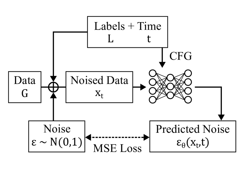
The diffusion model consists of two stages: (i) the diffusion process and (ii) the inverse process. In the diffusion process, noise is added to the input data and a machine learns to predict the added noise. In the inverse process, noise is gradually removed from a pure noise to generate meaningful data. In the context of flavor models, let us denote $G$ as free parameters in flavor models and $L$ as a conditional label specifying physical observables such as masses and mixings. For instance, the lepton sector was analyzed by incorporating the Yukawa couplings into $G$ and the neutrino masses and the PMNS matrix into $L$ in Ref. Nishimura:2025rsk . In this study, we aim to apply this method to the quark sector.

Based on an initial input data $x_{0}=G$ , a series of new data $\{x_{1},x_{2},\ldots,x_{T}\}$ is defined as Markov process that adds noise to the input $x_{0}$ :

	$\displaystyle q\left(x_{1:T}\|x_{0}\right)$	$\displaystyle=\prod_{t=1}^{T}q\left(x_{t}\|x_{t-1}\right),$		(2.1)
	$\displaystyle q\left(x_{t}\|x_{t-1}\right)$	$\displaystyle=\mathcal{N}\left(x_{t};\sqrt{A_{t}}x_{t-1},B_{t}\right),$		(2.2)

with $x_{i:j}=x_{i},x_{i+1},\ldots,x_{j}$ . Here, a conditional probability $q\left(x_{t}|x_{t-1}\right)$ denotes the probability of $x_{t}$ given the condition $x_{t-1}$ . In addition, $\mathcal{N}\left(x;\mu,\sigma\right)$ is a normal distribution with a random variable $x$ , an average $\mu$ , and a variance $\sigma$ . We will omit $x$ for brevity. $A_{t}$ is defined as $A_{t}=1-B_{t}$ , and the parameters $0<B_{1}<B_{2}<\cdots<B_{T}<1$ decide the variance of $\mathcal{N}$ . By the definition of $A$ and $B$ , the series of data close to pure noise that follows a standard normal distribution along with $t$ . Based on this property, $A_{t}$ and $B_{t}$ are referred to as noise schedules.

For practical purposes, the noised data at any given time is determined as

	$\displaystyle x_{t}$	$\displaystyle=\sqrt{\bar{A}_{t}}x_{0}+\sqrt{\bar{B}_{t}}\epsilon,$		(2.3)
	$\displaystyle\bar{A}_{t}$	$\displaystyle=\prod_{s=1}^{t}A_{s},\quad\bar{B}_{t}=1-\bar{A}_{t},$		(2.4)

with $t=1,\ldots,T$ . Here, $\epsilon$ is a noise obeying a standard normal distribution $\mathcal{N}\left(0,1\right)$ . Among the various ways to choose $B_{t}$ , we adopt a linear schedule:

\displaystyle B_{t}=\left(1-\frac{t}{T}\right)B_{\mathrm{min}}+\frac{t}{T}B_{\mathrm{max}}.

(2.5)

We adopt $B_{\mathrm{min}}=10^{-4}$ , $B_{\mathrm{max}}=0.02$ , and $T=1000$ .

Then, in the reverse process, pure noise $x_{T}$ from $\mathcal{N}\left(0,1\right)$ is prepared as initial data, and $x_{t-1}$ based on $x_{t}$ is sampled in sequence according to the following Markov process:

	$\displaystyle p_{\theta}\left(x_{0:T}\right)$	$\displaystyle=p\left(x_{T}\right)\prod_{t=1}^{T}p_{\theta}\left(x_{t-1}\|x_{t}\right),$		(2.6)
	$\displaystyle p\left(x_{T}\right)$	$\displaystyle=\mathcal{N}\left(x_{T};0,1\right).$		(2.7)

The conditional probability $p_{\theta}\left(x_{t-1}|x_{t}\right)$ at each step is estimated using a neural network, which is explained later, and characterized by parameters $\theta$ . In practice, sampling from $p_{\theta}$ corresponds to determining $x_{t-1}$ as follows:

	$\displaystyle x_{t-1}=\frac{1}{\sqrt{A_{t}}}\left(x_{t}-\frac{B_{t}}{\sqrt{\bar{B}_{t}}}\hat{\epsilon}_{\theta}\right)+\sigma_{t}u_{t},$		(2.8)
	$\displaystyle\hat{\epsilon}_{\theta}\left(x_{t},t,L\right)=\left(1-\gamma\right)\epsilon_{\theta}\left(x_{t},t\right)+\gamma\epsilon_{\theta}\left(x_{t},t,L\right),$		(2.9)

where $L$ is a conditional label and $u_{t}$ is a disturbance following $\mathcal{N}\left(0,1\right)$ . In addition, the coefficient $\gamma$ , which is called the CFG scale, satisfies the condition $\gamma\geq 0$ . A larger CFG scale means that the data are more faithful to the label $L$ , but the diversity of generated results tends to be lost. On the other hand, when $\gamma<1$ , it emphasizes the diversity. $\gamma=8$ is adopted in this study.

The predicted noise $\hat{\epsilon}_{\theta}$ is determined by a linear combination of the unlabeled noise and the labeled noise. In contrast to the expression of Eq. (2.9), just one mathematical model is required by considering $\epsilon_{\theta}(x_{t},t)=\epsilon_{\theta}(x_{t},t,L=\varnothing)$ . For practical training, $L=\varnothing$ is adopted with a low probability (10-20%), and the learning of CFG proceeds with mixing the cases with and without labels. For $\varnothing$ , a learned embedding vector or a zero vector $\varnothing=0$ is often used. In this study, we dropped out the labels in 10% of the cases, and 0 is used as $\varnothing$ in our study.

To predict the added noise, we utilize a neural network model in which a $n$ -th layer with $N_{n-1}$ dimensional vector $\vec{X}_{n-1}=(X_{n-1}^{1},\ldots,X_{n-1}^{N_{n-1}})$ transforms into a $N_{n}$ dimensional vector $\vec{X}_{n}=(X_{n}^{1},\ldots,X_{n}^{N_{n}})$ by following relation:

\displaystyle X_{n}^{i}=h_{n}\left(w^{ij}_{n}X_{n-1}^{j}+b^{i}_{n}\right),

(2.10)

where $h,w,b$ respectively denote the activation function, the weight and the bias. In general, the neural network realizes multiple nonlinear transformations through $h$ . In our architecture, a fully-connected network is adopted, and the network is trained by minimizing the mean squared error (MSE) loss representing the difference between the actual added noise $\epsilon$ and the predicted noise $\epsilon_{\theta}$ , as shown in Fig. 1. In the end, a well-trained network can accurately estimate the noise component in $x_{t}$ .

When we complete training a neural network once using initial data, the inverse process with that network can provide various new data $G$ including free parameters in flavor models. If the network does not reach the desired level of accuracy, many types of strategies are possible to tackle this problem. To enhance learning efficiency and accuracy, transfer learning is often applied by reusing a neural network that has already been learned. In a more narrowly defined method called fine-tuning, the parameters of the learned neural network are used as the initial values of a new neural network, and all parameters are updated based on other training data. This study also implements this method and evaluates its effectiveness. The details of transfer learning and fine-tuning are provided in Ref. Nishimura:2025rsk .

Refer to caption — Figure 1: The summary of input/output of a neural network in the diffusion process quoted from Ref. Nishimura:2025rsk . The neural network predicts an added noise based on the noised data and conditional labels.

3 $S_{4}^{\prime}$ modular flavor model as a case study

In this section, we apply the conditional diffusion model to a particular flavor model, namely the modular flavor model. By introducing the modular symmetry in Sec. 3.1, we present the $S_{4}^{\prime}$ modular flavor model in Sec. 3.2. The formulation of the conditional diffusion model is discussed in Sec. 3.3.

3.1 Modular symmetry

In this section, we review the $SL(2,\mathbb{Z})$ modular symmetry and introduce the $S_{4}^{\prime}$ modular flavor model. A principal congruence subgroup $\Gamma(N)$ of $SL(2,\mathbb{Z})$ is defined as follows:

\displaystyle\Gamma(N)=\left\{\begin{pmatrix}a&b\\ c&d\end{pmatrix}\in SL(2,\mathbb{Z}),\quad\begin{pmatrix}a&b\\ c&d\end{pmatrix}\equiv\begin{pmatrix}1&0\\ 0&1\end{pmatrix}\,\mathrm{mod}\,N\right\}.

(3.1)

This group acts on the complex variable $\tau$ called modulus ( $\imaginary\,[\tau]>0$ ) in the following way:

\displaystyle\tau\to\frac{a\tau+b}{c\tau+d},

(3.2)

with $ad-bc=1$ . In addition, $\Gamma(N)$ is generated by the three generators:

\displaystyle S=\begin{pmatrix}0&1\\ -1&0\end{pmatrix},\qquad T=\begin{pmatrix}1&1\\ 0&1\end{pmatrix},\qquad R=\begin{pmatrix}-1&0\\ 0&-1\end{pmatrix}.

(3.3)

These generators satisfy the following algebraic relations:

\displaystyle S^{2}=R,\qquad(ST)^{3}=R^{2}=\mathbb{I},\qquad TR=RT.

(3.4)

Using the definition of $\Gamma(N)$ , various finite modular groups are defined as follows:

$\displaystyle PSL(2,\mathbb{Z})$	$\displaystyle=SL(2,\mathbb{Z})/\mathbb{Z}_{2}^{R},$	(3.5)
$\displaystyle\Gamma_{N}^{\prime}$	$\displaystyle=SL(2,\mathbb{Z})/\Gamma(N),$	(3.6)
$\displaystyle\Gamma_{N}$	$\displaystyle=PSL(2,\mathbb{Z})/\Gamma(N).$	(3.7)

Note that $\Gamma_{N}$ with $N=2,3,4,5$ are isomorphic to $S_{3},A_{4},S_{4},A_{5}$ , respectively. Similarly, $\Gamma_{N}^{\prime}$ with $N=3,4,5$ are isomorphic to $A_{4}^{\prime},S_{4}^{\prime},A_{5}^{\prime}$ , which are double covering groups of $A_{4},S_{4},A_{5}$ , respectively. In these groups, the generator $T$ satisfies $T^{N}=\mathbb{I}$ , so it generates a $\mathbb{Z}_{N}^{T}$ symmetry.

In this paper, we focus on $S_{4}^{\prime}$ , having ten irreducible representations:

\displaystyle\mathbf{1},\mathbf{1}^{\prime},\mathbf{2},\mathbf{3},\mathbf{3}^{\prime}\quad\mathrm{and}\quad\hat{\mathbf{1}},\hat{\mathbf{1}}^{\prime},\hat{\mathbf{2}},\hat{\mathbf{3}},\hat{\mathbf{3}}^{\prime}.

(3.8)

The non-hatted and hatted representations respectively transform under $R$ trivially and non-trivially. In other words, $Rr=r$ and $R\hat{r}=-\hat{r}$ are satisfied for any representation $r$ and $\hat{r}$ . In this work, we choose representation matrices in which $T$ is diagonal and $S$ is real. For the doublet $\mathbf{2}$ and the triplet $\mathbf{3}$ , the representation matrices is chosen as follows Novichkov:2020eep :

	$\displaystyle\rho_{S}(\mathbf{2})=\frac{1}{2}\begin{pmatrix}-1&\sqrt{3}\\ \sqrt{3}&1\end{pmatrix},$	$\displaystyle\quad\rho_{T}(\mathbf{2})=\begin{pmatrix}1&0\\ 0&-1\end{pmatrix},$		(3.9)
	$\displaystyle\rho_{S}(\mathbf{3})=-\frac{1}{2}\begin{pmatrix}0&\sqrt{2}&\sqrt{2}\\ \sqrt{2}&-1&1\\ \sqrt{2}&1&-1\\ \end{pmatrix},$	$\displaystyle\quad\rho_{T}(\mathbf{3})=\begin{pmatrix}-1&0&0\\ 0&-i&0\\ 0&0&i\end{pmatrix}.$		(3.10)

Then, the primed/hatted representations obey following relations for any representation $r$ and $\hat{r}$ :

$\displaystyle\rho_{S}(r)$	$\displaystyle=-\rho_{S}(r^{\prime})=-i\rho_{S}(\hat{r})=i\rho_{S}(\hat{r}^{\prime}),$	(3.11)
$\displaystyle\rho_{T}(r)$	$\displaystyle=-\rho_{T}(r^{\prime})=i\rho_{T}(\hat{r})=-i\rho_{T}(\hat{r}^{\prime}),$	(3.12)
$\displaystyle\rho_{R}(r)$	$\displaystyle=\rho_{R}(r^{\prime})=-\rho_{R}(\hat{r})=-\rho_{R}(\hat{r}^{\prime})=1.$	(3.13)

In the upper half-plane in the complex plane of $\tau$ , a modular form $Y_{r}^{(k)}$ of representation $r$ with a weight $k$ is defined as a holomorphic function which transforms in the following rule under the modular symmetry:

\displaystyle Y_{r}^{(k)}(\tau)\to(c\tau+d)^{k}\rho(r)Y_{r}^{(k)}(\tau),

(3.14)

with a representation matrix $\rho(r)$ . In addition, a matter field $\phi$ is assumed to obey the same rule as follows:

\displaystyle\phi\to(c\tau+d)^{k_{\phi}}\rho(r_{\phi})\phi,

(3.15)

with representation $r_{\phi}$ and weight $k_{\phi}$ .

To present an explicit expression of the modular form under the $S_{4}^{\prime}$ modular symmetry, let us introduce the Dedekind eta function $\eta(\tau)$ :

\displaystyle\eta(\tau)=e^{\pi i\tau/12}\prod_{n=1}^{\infty}\left(1-e^{2\pi i\tau n}\right).

(3.16)

Using this, two functions $\theta$ and $\epsilon$ are defined as follows:

\displaystyle\begin{split}\theta(\tau)&=\frac{\eta(2\tau)^{5}}{\eta(\tau)^{2}\eta(4\tau)^{2}}=1+2\sum_{n=1}^{\infty}q^{n^{2}},\\ \epsilon(\tau)&=\frac{2\eta(4\tau)^{5}}{\eta(2\tau)}=2q^{1/4}\sum_{n=0}^{\infty}q^{n(n+1)},\end{split}

(3.17)

where we show their $q$ -expansions with $q=e^{2\pi i\tau}$ . Under the $S_{4}^{\prime}$ modular symmetry, there is a $\hat{\mathbf{3}}$ representation with $k_{Y}=1$ , which is referred to in Ref. Novichkov:2020eep :

\displaystyle Y^{(1)}_{\hat{\mathbf{3}}}(\tau)=\begin{pmatrix}\sqrt{2}\epsilon(\tau)\theta(\tau)\\ \epsilon^{2}(\tau)\\ -\theta^{2}(\tau)\end{pmatrix}.

(3.18)

Modular forms with higher weight are calculated by tensor products given in Ref. Novichkov:2020eep . In the following, we list relevant modular forms utilized in this work:

\displaystyle\begin{split}Y_{\mathbf{3}}^{(4)}&=\epsilon\theta(\epsilon^{4}-\theta^{4})\left(\begin{array}[]{c}-\sqrt{2}\epsilon\theta\\ -\epsilon^{2}\\ \theta^{2}\end{array}\right),\quad Y_{\mathbf{3}}^{(6)}=\epsilon\theta(\epsilon^{4}-\theta^{4})\left(\begin{array}[]{c}-2\sqrt{2}\epsilon\theta(\epsilon^{4}+\theta^{4})\\ \epsilon^{2}(\epsilon^{4}-5\theta^{4})\\ \theta^{2}(5\epsilon^{4}-\theta^{4})\end{array}\right),\\ Y_{\mathbf{3}}^{1,(8)}&=\epsilon\theta(\epsilon^{4}-\theta^{4})\left(\begin{array}[]{c}16\sqrt{2}\epsilon^{5}\theta^{5}\\ \epsilon^{2}(\epsilon^{8}+10\epsilon^{4}\theta^{4}+5\theta^{8})\\ -\theta^{2}(5\epsilon^{8}+10\epsilon^{4}\theta^{4}+\theta^{8})\end{array}\right),\\ Y_{\mathbf{3}}^{2,(8)}&=\epsilon^{2}\theta^{2}(\epsilon^{4}-\theta^{4})^{2}\left(\begin{array}[]{c}\epsilon^{4}-\theta^{4}\\ 2\sqrt{2}\epsilon\theta^{3}\\ 2\sqrt{2}\epsilon^{3}\theta\end{array}\right),\\ Y_{\hat{\mathbf{3}}}^{1,(7)}&=\left(\begin{array}[]{c}32\sqrt{2}\epsilon^{5}\theta^{5}(\epsilon^{4}+\theta^{4})\\ -\epsilon^{2}(\epsilon^{12}-19\epsilon^{8}\theta^{4}-45\epsilon^{4}\theta^{8}-\theta^{12})\\ -\theta^{2}(\epsilon^{12}+45\epsilon^{8}\theta^{4}+19\epsilon^{4}\theta^{8}-\theta^{12})\end{array}\right),\\ Y_{\hat{\mathbf{3}}}^{2,(7)}&=\epsilon\theta(\epsilon^{4}-\theta^{4})\left(\begin{array}[]{c}\epsilon^{8}-\theta^{8}\\ -\sqrt{2}\epsilon\theta^{3}(7\epsilon^{4}+\theta^{4})\\ -\sqrt{2}\epsilon^{3}\theta(\epsilon^{4}+7\theta^{4})\end{array}\right).\end{split}

(3.19)

3.2 Quark sector

Then, we consider a specific example of $S_{4}^{\prime}$ modular flavor model with an emphasis on the quark sector. Following Ref. Abe:2023qmr , we suppose that $Q$ is a triplet representation of $S_{4}^{\prime}$ , $\{u_{1}^{c},u_{2}^{c},d_{1}^{c},d_{2}^{c},d_{3}^{c}\}$ are trivial singlets of $S_{4}^{\prime}$ , and $u_{3}^{c}$ are the non-trivial singlets of $S_{4}^{\prime}$ , i.e.,

\displaystyle Q\,:\,\mathbf{3},\qquad u^{c}\,:\,\mathbf{1}\oplus\mathbf{1}\oplus\hat{\mathbf{1}}^{\prime},\qquad d^{c}\,:\,\mathbf{1}\oplus\mathbf{1}\oplus\mathbf{1}.

(3.20)

In addition, Higgs doublets $H_{u}$ and $H_{d}$ are considered trivial singlets $\mathbf{1}$ . These assignments are summarized in Table 1. In the previous study, it was investigated that the CKM matrix has diagonal textures by this configuration.

	$Q$	$u_{1}^{c}$	$u_{2}^{c}$	$u_{3}^{c}$	$d_{1}^{c}$	$d_{2}^{c}$	$d_{3}^{c}$	$H_{u}$	$H_{d}$
$S_{4}^{\prime}$	$\mathbf{3}$	$\mathbf{1}$	$\mathbf{1}$	$\hat{\mathbf{1}}^{\prime}$	$\mathbf{1}$	$\mathbf{1}$	$\mathbf{1}$	$\mathbf{1}$	$\mathbf{1}$
Weight	$-4$	$0$	$-4$	$-3$	$0$	$-2$	$-4$	0	0

Table 1: Assignments of representation for the quarks and Higgs doublets and modular weights.

Under this setup, the superpotential in the quark sector is given by

	$\displaystyle W_{q}=$	$\displaystyle H_{u}\left\{\alpha_{1}(QY_{\mathbf{3}}^{(4)})_{\mathbf{1}}u_{1}^{c}+\sum_{a=1}^{2}\left[\alpha_{2}^{a}(QY_{\mathbf{3}}^{a,(8)})_{\mathbf{1}}u_{2}^{c}+\alpha_{3}^{a}((QY_{\hat{\mathbf{3}}}^{a,(7)})_{\hat{\mathbf{1}}}u_{3}^{c})_{\mathbf{1}}\right]\right\}$
		$\displaystyle+H_{d}\left\{\beta_{1}(QY_{\mathbf{3}}^{(4)})_{\mathbf{1}}d_{1}^{c}+\beta_{2}(QY_{\mathbf{3}}^{(6)})_{\mathbf{1}}d_{2}^{c}+\sum_{a=1}^{2}\beta_{3}^{a}(QY_{\mathbf{3}}^{a,(8)})_{\mathbf{1}}d_{3}^{c}\right\}.$		(3.21)

In each term, $(\cdots)_{\mathbf{1}}$ is a trivial singlet among the results of the tensor product in the parentheses. The products of the triplet representations are given by

	$\displaystyle(\mathbf{3}(\phi)\otimes\mathbf{3}(\psi))_{1}$	$\displaystyle=\phi_{1}\psi_{1}+\phi_{2}\psi_{3}+\phi_{3}\psi_{2},$		(3.22)
	$\displaystyle(\mathbf{3}(\phi)\otimes\hat{\mathbf{3}}(\psi))_{\hat{1}}$	$\displaystyle=\phi_{1}\psi_{1}+\phi_{2}\psi_{3}+\phi_{3}\psi_{2}.$		(3.23)

Then, mass terms of the up-type quarks are derived as follows:

	$\displaystyle\langle H_{u}\rangle\left\{\alpha_{1}\left(Q_{1}(Y_{\mathbf{3}}^{(4)})_{1}+Q_{2}(Y_{\mathbf{3}}^{(4)})_{3}+Q_{3}(Y_{\mathbf{3}}^{(4)})_{2}\right)u_{1}^{c}\right\}$
	$\displaystyle+\langle H_{u}\rangle\left\{\sum_{a=1}^{2}\alpha_{2}^{a}\left(Q_{1}(Y_{\mathbf{3}}^{a,(8)})_{1}+Q_{2}(Y_{\mathbf{3}}^{a,(8)})_{3}+Q_{3}(Y_{\mathbf{3}}^{a,(8)})_{2}\right)\right\}u_{2}^{c}$
	$\displaystyle+\langle H_{u}\rangle\left\{\sum_{a=1}^{2}\alpha_{3}^{a}\left(Q_{1}(Y_{\hat{\mathbf{3}}}^{a,(7)})_{1}+Q_{2}(Y_{\hat{\mathbf{3}}}^{a,(7)})_{3}+Q_{3}(Y_{\hat{\mathbf{3}}}^{a,(7)})_{2}\right)\right\}u_{3}^{c},$		(3.24)

i.e.,

\displaystyle M_{u}=\langle H_{u}\rangle\begin{pmatrix}\alpha_{1}(Y_{\mathbf{3}}^{(4)})_{1},&\alpha_{2}^{1}(Y_{\mathbf{3}}^{1,(8)})_{1}+\alpha_{2}^{2}(Y_{\mathbf{3}}^{2,(8)})_{1},&\alpha_{3}^{1}(Y_{\hat{\mathbf{3}}}^{1,(7)})_{1}+\alpha_{3}^{2}(Y_{\hat{\mathbf{3}}}^{2,(7)})_{1}\\ \alpha_{1}(Y_{\mathbf{3}}^{(4)})_{3},&\alpha_{2}^{1}(Y_{\mathbf{3}}^{1,(8)})_{3}+\alpha_{2}^{2}(Y_{\mathbf{3}}^{2,(8)})_{3},&\alpha_{3}^{1}(Y_{\hat{\mathbf{3}}}^{1,(7)})_{3}+\alpha_{3}^{2}(Y_{\hat{\mathbf{3}}}^{2,(7)})_{3}\\ \alpha_{1}(Y_{\mathbf{3}}^{(4)})_{2},&\alpha_{2}^{1}(Y_{\mathbf{3}}^{1,(8)})_{2}+\alpha_{2}^{2}(Y_{\mathbf{3}}^{2,(8)})_{2},&\alpha_{3}^{1}(Y_{\hat{\mathbf{3}}}^{1,(7)})_{2}+\alpha_{3}^{2}(Y_{\hat{\mathbf{3}}}^{2,(7)})_{2}\\ \end{pmatrix}.

(3.25)

In the same way, mass terms of the down-type quarks are derived as follows:

	$\displaystyle\langle H_{d}\rangle\left\{\beta_{1}\left(Q_{1}(Y_{\mathbf{3}}^{(4)})_{1}+Q_{2}(Y_{\mathbf{3}}^{(4)})_{3}+Q_{3}(Y_{\mathbf{3}}^{(4)})_{2}\right)d_{1}^{c}\right\}$
	$\displaystyle+\langle H_{d}\rangle\left\{\beta_{2}\left(Q_{1}(Y_{\mathbf{3}}^{(6)})_{1}+Q_{2}(Y_{\mathbf{3}}^{(6)})_{3}+Q_{3}(Y_{\mathbf{3}}^{(6)})_{2}\right)d_{2}^{c}\right\}$
	$\displaystyle+\langle H_{d}\rangle\left\{\sum_{a=1}^{2}\beta_{3}^{a}\left(Q_{1}(Y_{\mathbf{3}}^{a,(8)})_{1}+Q_{2}(Y_{\mathbf{3}}^{a,(8)})_{3}+Q_{3}(Y_{\mathbf{3}}^{a,(8)})_{2}\right)\right\}d_{3}^{c},$		(3.26)

i.e.,

\displaystyle M_{d}=\langle H_{d}\rangle\begin{pmatrix}\beta_{1}(Y_{\mathbf{3}}^{(4)})_{1},&\beta_{2}(Y_{\mathbf{3}}^{(6)})_{1},&\beta_{3}^{1}(Y_{\mathbf{3}}^{1,(8)})_{1}+\beta_{3}^{2}(Y_{\mathbf{3}}^{2,(8)})_{1}\\ \beta_{1}(Y_{\mathbf{3}}^{(4)})_{3},&\beta_{2}(Y_{\mathbf{3}}^{(6)})_{3},&\beta_{3}^{1}(Y_{\mathbf{3}}^{1,(8)})_{3}+\beta_{3}^{2}(Y_{\mathbf{3}}^{2,(8)})_{3}\\ \beta_{1}(Y_{\mathbf{3}}^{(4)})_{2},&\beta_{2}(Y_{\mathbf{3}}^{(6)})_{2},&\beta_{3}^{1}(Y_{\mathbf{3}}^{1,(8)})_{2}+\beta_{3}^{2}(Y_{\mathbf{3}}^{2,(8)})_{2}\\ \end{pmatrix}.

(3.27)

The Kähler potential of the chiral superfield $\phi_{i}$ is written as follows:

\displaystyle K\supset\sum_{i}\frac{\phi_{i}^{\dagger}\phi_{i}}{\left(-i\tau+i\bar{\tau}\right)^{k_{\phi_{i}}}},

(3.28)

where $-k_{\phi_{i}}$ is a weight of the superfield. Thus, each component of the mass matrices is modified by the canonical normalization as

\displaystyle\left(M_{\phi}\right)_{ij}\to\left(\sqrt{2\imaginary\,[\tau]}\right)^{k_{Q}+k_{\phi_{j}}}\left(M_{\phi}\right)_{ij},

(3.29)

with $i,j=1,2,3$ and $\phi=u,d$ .

The mass matrices are diagonalized by unitary matrices as follows:

	$\displaystyle M_{u}$	$\displaystyle=U_{L}^{\dagger}\mathrm{diag}(m_{u},m_{c},m_{t})U_{R},$		(3.30)
	$\displaystyle M_{d}$	$\displaystyle=V_{L}^{\dagger}\mathrm{diag}(m_{d},m_{s},m_{b})V_{R}.$		(3.31)

Moreover, the flavor mixing is defined as the difference between mass eigenstates and flavor eigenstates:

	$\displaystyle U_{\mathrm{CKM}}$	$\displaystyle=U_{L}V_{L}^{\dagger}$
		$\displaystyle=\begin{pmatrix}c_{12}c_{13}&s_{12}c_{13}&s_{13}e^{-i\delta_{\rm{CP}}}\\ -s_{12}c_{23}-c_{12}s_{23}s_{13}e^{i\delta_{\rm{CP}}}&c_{12}c_{23}-s_{12}s_{23}s_{13}e^{i\delta_{\rm{CP}}}&s_{23}c_{13}\\ s_{12}s_{23}-c_{12}c_{23}s_{13}e^{i\delta_{\rm{CP}}}&-c_{12}s_{23}-s_{12}c_{23}s_{13}e^{i\delta_{\rm{CP}}}&c_{23}c_{13}\end{pmatrix},$		(3.32)

with $c_{ij}=\cos{\theta_{ij}}$ and $s_{ij}=\sin{\theta_{ij}}$ . Moreover, the Jarlskog invariant is defined as follows:

\displaystyle J=\imaginary\,\left[U_{11}U_{22}U_{12}^{*}U_{21}^{*}\right]=s_{23}c_{23}s_{12}c_{12}s_{13}c_{13}^{2}\sin{\delta_{\mathrm{CP}}},

(3.33)

which is a measure of CP violation.

At $\tan\beta=10$ and the SUSY breaking scale $M_{\mathrm{SUSY}}=10\,\mbox{TeV}$ , we show values of masses and mixings in Table 2, which is calculated from Ref. Antusch:2013jca . In addition, from mixing angles in that data, absolute values of the CKM matrix is derived as follows:

\displaystyle|U_{\mathrm{CKM}}|=\left(\begin{array}[]{ccc}0.9743\pm 0.0002&0.2254\pm 0.0007&0.0035\pm 0.0001\\ 0.2253\pm 0.0007&0.9735\pm 0.0002&0.0401\pm 0.0006\\ 0.0085\pm 0.0002&0.0394\pm 0.0006&0.9992\pm 0.0000\\ \end{array}\right).

(3.37)

From an analytical point of view, $\theta(\tau)\sim 1$ and $\epsilon(\tau)\sim 2q^{1/4}\ll 1$ when $2\pi\imaginary\,[\tau]\gg 1$ . This makes the hierarchical structure of mass matrices Eq. (3.25) and Eq. (3.27), so it is easy to realize semi-realistic flavor structure. It is non-trivial how small $\imaginary\,[\tau]$ is allowed to reproduce the flavor structure, and $\imaginary\,[\tau]\sim 2.8$ was found as one of the optimal values in Ref. Abe:2023qmr .

	$\mu_{i}\pm 1\sigma$
$\left(m_{u}/m_{t}\right)/10^{-6}$	$5.4412\pm 1.7132$
$\left(m_{c}/m_{t}\right)/10^{-3}$	$2.8213\pm 0.1195$
$m_{t}/\mbox{GeV}$	$87.4555$
$\left(m_{d}/m_{b}\right)/10^{-4}$	$9.2159\pm 1.2382$
$\left(m_{s}/m_{b}\right)/10^{-2}$	$1.8241\pm 0.1005$
$m_{b}/\mbox{GeV}$	$0.9682$
$s_{12}^{q}/10^{-1}$	$2.2736\pm 0.0073$
$s_{23}^{q}/10^{-2}$	$4.015\pm 0.064$
$s_{13}^{q}/10^{-3}$	$3.49\pm 0.13$
$\delta_{\text{CKM}}/\pi$	$0.3845\pm 0.0173$
$J/10^{-5}$	$2.87\pm 0.13$

Table 2: The central values and

1\sigma

ranges for the quark sector with

\tan\beta=10

and

M_{\mathrm{SUSY}}=10\,\mbox{TeV}

based on Ref. Antusch:2013jca .

3.3 Conditional diffusion model

In this section, we present the detailed design of the conditional diffusion model adopted for the $S_{4}^{\prime}$ modular flavor model as a case study. The diffusion process, the inverse process, and the transfer learning will be described in this order.

Diffusion process

We adopt $\tan\beta=10.0,\,\alpha_{3}^{1}=0.001$ . In preparing the initial data, we deal with the following values ^*^**In our analysis, the modulus field $\tau$ (symmetry breaking field) is regarded as a parameter, but the VEV of $\tau$ will be determined by its stabilization mechanism proposed in e.g., Ishiguro:2020tmo ; Novichkov:2022wvg ; Ishiguro:2022pde .:

	$\displaystyle G$	$\displaystyle=\left\{\frac{\alpha_{1}}{10\cdot\alpha_{3}^{1}},\,\frac{\alpha_{2}^{1}}{10\cdot\alpha_{3}^{1}},\,\frac{\alpha_{2}^{2}}{10\cdot\alpha_{3}^{1}},\,\frac{\alpha_{3}^{2}}{10\cdot\alpha_{3}^{1}},\,\frac{\beta_{1}}{10\cdot\alpha_{3}^{1}},\,\frac{\beta_{2}}{10\cdot\alpha_{3}^{1}},\,\frac{\beta_{3}^{1}}{10\cdot\alpha_{3}^{1}},\,\frac{\beta_{3}^{2}}{10\cdot\alpha_{3}^{1}},\,\real\,[\tau],\,\imaginary\,[\tau]\right\},$		(3.38)
	$\displaystyle L$	$\displaystyle=\left\{\log_{10}\frac{m_{u}}{m_{t}},\,\log_{10}\frac{m_{c}}{m_{t}},\,0.0,\,\log_{10}\frac{m_{d}}{m_{b}},\,\log_{10}\frac{m_{s}}{m_{b}},\,0.0,\,\|(U_{\rm CKM})_{ij}\|,\,\mathrm{sign}[J]\times\log_{10}\|J\|\right\},$		(3.39)

with $i,j=1,2,3$ . For $L$ , we introduce trivial labels to represent $\log_{10}(m_{t}/m_{t})$ and $\log_{10}(m_{b}/m_{b})$ . These dummy labels allow the dimensions of $L$ to be matched to a number of independent physical quantities, which is beneficial for developing a generic architecture of the neural network. However, it remains uncertain whether these dummy labels enhance learning accuracy. The necessity of these dummy labels will be reported elsewhere. In addition, we avoid exponential differences in the input values to the neural network by applying the logarithm to the mass ratio and the Jarlskog invariant.

Now, $G$ has 10 components and $L$ has 16 components. Each element of $G$ was generated as uniform random numbers satisfying the following ranges:

$\displaystyle 0.01$	$\displaystyle\leq\left\{\left\|\frac{\alpha_{1}}{10\cdot\alpha_{3}^{1}}\right\|,\,\left\|\frac{\alpha_{2}^{1}}{10\cdot\alpha_{3}^{1}}\right\|,\,\left\|\frac{\alpha_{2}^{2}}{10\cdot\alpha_{3}^{1}}\right\|,\,\left\|\frac{\alpha_{3}^{2}}{10\cdot\alpha_{3}^{1}}\right\|\right\}\leq 1.0,$	(3.40)
$\displaystyle 0.01$	$\displaystyle\leq\left\{\left\|\frac{\beta_{1}}{10\cdot\alpha_{3}^{1}}\right\|,\,\left\|\frac{\beta_{2}}{10\cdot\alpha_{3}^{1}}\right\|,\,\left\|\frac{\beta_{3}^{1}}{10\cdot\alpha_{3}^{1}}\right\|,\,\left\|\frac{\beta_{3}^{2}}{10\cdot\alpha_{3}^{1}}\right\|\right\}\leq 1.0,$	(3.41)
$\displaystyle-\frac{1}{2}$	$\displaystyle\leq\real\,[\tau]\leq\frac{1}{2},\quad\frac{\sqrt{3}}{2}\leq\imaginary\,[\tau]\leq 5.0.$	(3.42)

Eq. (3.40) and Eq. (3.41) mean that the ratios of coefficients $r$ satisfy $0.1\leq|r|\leq 10$ . In addition, data processing techniques such as normalization and standardization are important for achieving efficient learning of neural networks. In this respect, the ratio $r$ in the component of $G$ is divided by ten to realize the proper normalization $r\sim\mathcal{O}(1)$ .

Then, $L$ is computed from a randomly generated $G$ based on Eq. (3.25) and Eq. (3.27), and a neural network is trained using pairs of the input and the label $x_{0}=\left(G,L\right)$ . In actual learning process, we prepare $10^{5}$ pairs of $\left(G,L\right)$ as initial data. Of these data, 90% are used as training data and 10% as validation data. When the integer $t$ is randomly selected from $[1,T]$ , the noisy data $x_{t}$ is determined according to Eq. (2.4). When an input layer of the neural network receives $x_{t}$ as input, it performs nonlinear transformations according to Eq. (2.10).

The detailed architecture of our neural network is presented in Table 3. There are 646,836 parameters that are adjusted during training. The activation function $h$ in Eq. (2.10) is selected as the SELU function for hidden layers and an identity function for an output layer. The batch size is set to 64, and the parameter updates are performed $10^{5}$ times. In addition, we employ the ADAM optimizer in PyTorch to update the weight $w$ and bias $b$ described in Eq. (2.10). The learning rate is automatically adjusted using the scheduler “OneCycleLR” provided by PyTorch, and we adopted $r_{\mathrm{max}}=0.001$ as the maximum rate.

Layer	Dimension	Activation	Layer	Dimension	Activation
Input	$\mathbb{R}^{10}_{x}+\mathbb{R}^{17}_{L,t}$	-	Hidden 6	$\mathbb{R}^{512}+\mathbb{R}^{17}_{L,t}$	SELU
Hidden 1	$\mathbb{R}^{32}+\mathbb{R}^{17}_{L,t}$	SELU	Hidden 7	$\mathbb{R}^{256}+\mathbb{R}^{17}_{L,t}$	SELU
Hidden 2	$\mathbb{R}^{64}+\mathbb{R}^{17}_{L,t}$	SELU	Hidden 8	$\mathbb{R}^{128}+\mathbb{R}^{17}_{L,t}$	SELU
Hidden 3	$\mathbb{R}^{128}+\mathbb{R}^{17}_{L,t}$	SELU	Hidden 9	$\mathbb{R}^{64}+\mathbb{R}^{17}_{L,t}$	SELU
Hidden 4	$\mathbb{R}^{256}+\mathbb{R}^{17}_{L,t}$	SELU	Hidden 10	$\mathbb{R}^{32}+\mathbb{R}^{17}_{L,t}$	SELU
Hidden 5	$\mathbb{R}^{512}+\mathbb{R}^{17}_{L,t}$	SELU	Output	$\mathbb{R}^{10}$	Identity

Table 3: In the neural network, the inputs are the noised data

x_{t}

(10 dimensions), the label

L

(16 dimensions), and the time

t

. The activation functions are the SELU function for hidden layers and the identity function for the output layer.

L

is treated as

\varnothing

in probability of 10%.

Reverse process

In the reverse process, the generation is performed with labels that reflect real observables. In particular, $L$ is designated as follows based on Table 2 and Eq. (3.37):

\displaystyle\begin{split}&\log_{10}\frac{m_{u}}{m_{t}}=\log_{10}\left(5.4412\times 10^{-6}\right)=-5.2643,\\ &\log_{10}\frac{m_{c}}{m_{t}}=\log_{10}\left(2.8213\times 10^{-3}\right)=-2.5496,\\ &\log_{10}\frac{m_{d}}{m_{b}}=\log_{10}\left(9.2159\times 10^{-4}\right)=-3.0355,\\ &\log_{10}\frac{m_{s}}{m_{b}}=\log_{10}\left(1.8241\times 10^{-2}\right)=-1.7390,\\ &|(U_{\rm CKM})_{ij}|=\left(\begin{array}[]{ccc}0.9743&0.2254&0.0035\\ 0.2253&0.9735&0.0401\\ 0.0085&0.0394&0.9992\\ \end{array}\right),\\ &\mathrm{sign}[J]\times\log_{10}|J|=+\log_{10}\left(2.87\times 10^{-5}\right)=-4.54.\end{split}

(3.43)

Then, $L$ is recalculated using the generated $G$ , and the data that falls within a specified error range is extracted. As a result, the data $G$ corresponding to the experimental values has been derived solely from the experimental label.

Transfer learning

After the diffusion model generates the data $G$ , the physical values $P_{\ell}$ corresponding to $G$ can be calculated. The accuracy of $P_{\ell}$ in comparison to the target experimental label $L$ is quantitatively evaluated by the $\chi^{2}$ value defined as follows:

\displaystyle\chi^{2}=\sum_{\ell=1}^{n}\left(\frac{P_{\ell}-\mu_{\ell}}{\sigma_{\ell}}\right)^{2},

(3.44)

where $P_{\ell},\mu_{\ell},\sigma_{\ell}$ respectively denote prediction for physical observable, central value and $1\sigma$ deviations. In this work, the $\chi^{2}$ function is calculated for following 8 observables:

\displaystyle\left\{\frac{m_{u}}{m_{t}},\,\frac{m_{c}}{m_{t}},\,\frac{m_{d}}{m_{b}},\,\frac{m_{s}}{m_{b}},\,\theta_{12}^{q},\,\theta_{23}^{q},\,\theta_{13}^{q},\,\left|\frac{\delta_{\mathrm{CKM}}}{\pi}\right|\right\},

(3.45)

so the CP violation is considered in $\chi^{2}$ .

Now, we refer to the first neural network as a pre-network. The data generated by the pre-network are collected for transfer learning, and the pre-network is retrained based on this new data. All parameters of the pre-network are updated, which is why the second training phase is referred to as fine-tuning. In our training process, the hyperparameters during the second phase are the same as those used in the first phase. The second network constructed through fine-tuning is referred to as a tuned-network in the following discussion.

4 Results

Our calculations are performed using Google Colaboratory with a CPU (not a GPU), so this method accessible to everyone. The diffusion process takes approximately 1 hour, and the reverse process requires approximately 4.6 hours per generating $10^{5}$ data in a single session. First, we generate data using a pre-network. The total number of data generated by the network is $4\times 10^{6}$ , of which 103,663 satisfy the condition $\chi^{2}<8.0\times 10^{4}$ . Therefore, in the diffusion model without fine-tuning, the ratio of data satisfying condition $\chi^{2}<8.0\times 10^{4}$ is 2.59%. Second, we perform fine-tuning on the 103,663 data generated by the pre-network that satisfy condition $\chi^{2}<8.0\times 10^{4}$ . When we generate a total of $9\times 10^{6}$ data using the tuned-network, there are 17 solutions that satisfy the condition $\chi^{2}<200.0$ . Here, in the diffusion model with fine-tuning, the ratio of data satisfying condition $\chi^{2}<8.0\times 10^{4}$ is 5.95%. Finally, we extract 11 solutions such that the CP phase is positive.

Based on these results, the accuracy of the data has improved through fine-tuning. In other words, fine-tuning enables the diffusion model to reproduce experimental values with greater precision. Furthermore, since the architectures of both the pre-network and the tuned-network are identical, the enhancement in accuracy can be achieved simply by repeating the learning process. Consequently, this method of improvement can be applied irrespective of the specific details of the flavor model. It is also anticipated that fine-tuning can be repeated to achieve the desired level of accuracy.

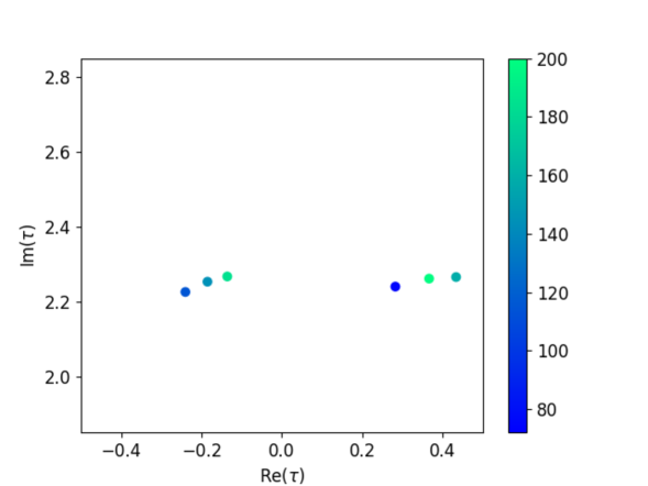
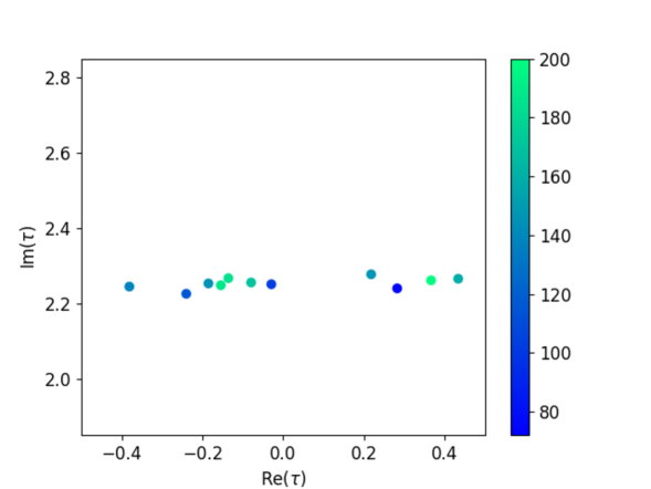
To show the progress of the generation process, Fig. 2 presents three graphs depicting the distribution of modulus $\tau$ as the amount of generated data increases. We observed a growing number of candidates that reproduce the flavor structure of the quarks with $\chi^{2}<200$ . In fact, phenomenologically promising candidates of $\tau$ appear in various locations, particularly concentrated around $\imaginary\,[\tau]\sim 2.2$ . The values of the data $G$ corresponding to the solution with the lowest $\chi^{2}$ value are as follows:

\displaystyle\begin{split}&\frac{\alpha_{1}}{\alpha_{3}^{1}}=0.0386,\,\frac{\alpha_{2}^{1}}{\alpha_{3}^{1}}=0.0479,\,\frac{\alpha_{2}^{2}}{\alpha_{3}^{1}}=0.4705,\,\frac{\alpha_{3}^{2}}{\alpha_{3}^{1}}=-1.1378,\\ &\frac{\beta_{1}}{\alpha_{3}^{1}}=-4.3717,\,\frac{\beta_{2}}{\alpha_{3}^{1}}=-0.2171,\,\frac{\beta_{3}^{1}}{\alpha_{3}^{1}}=2.8057,\,\frac{\beta_{3}^{2}}{\alpha_{3}^{1}}=-7.5297,\\ &\real\,[\tau]=0.2825,\quad\imaginary\,[\tau]=2.2400.\end{split}

(4.1)

These parameters lead to the following observables within $\chi^{2}=74.4$ .

\displaystyle\begin{split}\left(\frac{m_{u}}{m_{t}}\big{/}10^{-6},\,\frac{m_{c}}{m_{t}}\big{/}10^{-3}\right)&=\left(0.949,\,3.12\right),\\ \left(\frac{m_{d}}{m_{b}}\big{/}10^{-4},\,\frac{m_{s}}{m_{b}}\big{/}10^{-2}\right)&=\left(10.6,\,1.85\right),\\ \left(s_{12}^{q}/10^{-1},\,s_{23}^{q}/10^{-2},\,s_{13}^{q}/10^{-3},\,\delta_{\mathrm{CKM}}/\pi\right)&=\left(2.24,\,4.14,\,3.6,\,0.482\right).\end{split}

(4.2)

As mentioned above, this study confirmed that the accuracy of the generated results can be enhanced by performing the transfer learning only once. In order to reproduce the experimental values with even greater precision, it may be beneficial not only to conduct transfer learning multiple times but also to combine conventional methods, such as the Monte-Carlo method, with the parameters proposed by the diffusion model. The superiority of either approach remains to be investigated, and a comparison of their effectiveness taking into account computational resources should be reserved for future research.

As described in Sec. 3.2, the flavor structure in the $S_{4}^{\prime}$ modular flavor model strongly depends on $\imaginary\,[\tau]$ . When $\imaginary\,[\tau]$ is large, it is easy to reproduce the semi-realistic flavor structure. On the other hand, in regions where $\imaginary\,[\tau]$ is small, estimating the appropriate $\imaginary\,[\tau]$ becomes challenging, as even a slight variation can lead to a significantly different flavor structure. As a result, analytic evaluation with small $\imaginary\,[\tau]$ is a difficult issue. The diffusion model that we developed does not impose strict restrictions on the parameter regions to be explored and generates a variety of candidates across a broad search range. Because of this property, there is no need for human beings to adjust the search region of parameters. Under these circumstances, the fact that the solutions have smaller $\imaginary\,[\tau]$ than those in previous studies indicates that the diffusion model can find out characteristics of flavor models that are difficult to capture using conventional methods.

We now discuss the physical implications of the 11 results generated by the diffusion model. Table 4 summarizes the values of $\tau$ and the Jarlskog invariant for each result. In particular, the median value of the Jarlskog invariant is $2.49\times 10^{-5}$ , which is comparable in magnitude to the experimental value $2.87\times 10^{-5}$ . Various previous studies addressing the $S_{4}^{\prime}$ modular flavor models often introduce the coefficients $\{\alpha,\beta\}$ as complex numbers to reproduce a Jarlskog invariant of reasonable size. In contrast, this study treats the parameters $\{\alpha,\beta\}$ as real numbers, and the Jarlskog invariant is reproduced from only $\real\,[\tau]$ . Thus, the spontaneous CP violation can be realized in the $S_{4}^{\prime}$ modular flavor model. By broadly exploring the parameter space, the diffusion model can reveal new properties of the $S_{4}^{\prime}$ model that are difficult to discover through human experience alone.

$\real\,[\tau]$	$0.367$	$-0.185$	$-0.136$	$0.434$	$\mathbf{0.283}$
$\imaginary\,[\tau]$	$2.26$	$2.25$	$2.27$	$2.27$	$\mathbf{2.24}$
$J/10^{-5}$	$2.43$	$1.86$	$1.63$	$1.47$	$\mathbf{3.26}$
$\real\,[\tau]$	$-0.240$	$-0.155$	$0.218$	$-0.079$	$-0.029$	$-0.381$
$\imaginary\,[\tau]$	$2.23$	$2.25$	$2.28$	$2.26$	$2.25$	$2.24$
$J/10^{-5}$	$2.48$	$2.91$	$3.01$	$2.49$	$3.07$	$3.74$

Table 4: The values of modulus

\tau

and Jarlskog invariant for the 11 solutions generated by the diffusion model. The bold numbers show a result with the smallest

\chi^{2}

value shown in Eq. (4.1).

5 Conclusions

In order to understand the flavor structure of elementary particles, it is important to deepen our understanding of flavor models. Specifically, if we can find parameters that not only reproduce known observables but also reveal undiscovered properties, we can analyze the underlying structure of flavor models. In this study, we focused on the $S_{4}^{\prime}$ modular flavor model as a specific application of the diffusion model, a type of generative AI, and searched free parameters that reproduce experimental results. Conventional numerical methods typically require optimization by repeating the process to find out the desirable experimental values around fixed parameters as in the Monte-Carlo method. In contrast to those traditional approaches, the diffusion model provides a framework that is independent of the specific details of flavor models. Furthermore, it enables an inverse problem approach in which the machine provides a series of plausible model parameters from given experimental data. The diffusion models can serve as a versatile analytical tool for extracting new physical predictions from flavor models.

In this paper, we constructed a diffusion model with CFG to analyze the flavor structure of the quarks in the modular flavor model. Sec. 2 introduced the diffusion models and transfer learning in order to apply it to some flavor models. In Sec. 3, the $S_{4}^{\prime}$ modular flavor model was used as a concrete example, and the diffusion model was applied to search for its free parameters. Following a brief review of the $S_{4}^{\prime}$ modular symmetry in Sec. 3.1, we organized the description of the quark sector of the $S_{4}^{\prime}$ model in Sec. 3.2. Specific representations and weights are selected based on the previous study to reproduce the semi-realistic flavor structure, so observables can be calculated by determining the free parameters. To optimize these parameters, the setup of our diffusion model is introduced in Sec. 3.3, and physical implications derived from the data obtained by the diffusion model are discussed in Sec. 4.

Specifically, we confirmed that the accuracy of the data generated by the diffusion model is indeed improved through the transfer learning, and exhibited how various parameter solutions are found as the number of data is increased. The generated results indicated that $\imaginary\,[\tau]$ was concentrated in a smaller region than in the previous study. Furthermore, it was found that the spontaneous CP violation appeared in the $S_{4}^{\prime}$ modular flavor model from $\real\,[\tau]$ . These findings demonstrate that the diffusion model can find semi-realistic parameters via experimental observables. In conclusion, the diffusion model has significant potential for analyzing flavor models independently of the specific details of the models.

Before closing our paper, we will mention possible future works:

•

Although our analysis considers only the quark sector, the lepton sector can also be analyzed by the same procedure. Even within a framework that addresses both quarks and leptons simultaneously, there is no significant difference except that the inputs and outputs of the neural network have approximately double the dimensions. Due to this characteristic, a search for free parameters in other modular flavor models can also be anticipated as a direct extension.
•

The representation and modular weights of the fields used in this study were determined from an analytical perspective to achieve semi-realistic flavor structure and were fixed at specific values. In the future, the application of machine learning could automate the selection of the expressions and weights themselves. In fact, reinforcement learning, which is a type of machine learning, was utilized to search for $U(1)$ charges to assign to the fields in Refs. Harvey:2021oue ; Nishimura:2023nre ; Nishimura:2024apb . By combining such techniques with diffusion models, it is possible to find out predictions of flavor models that have not been identified in previous empirical studies.
•

In light of the two aforementioned prospects, it is expected that various flavor models will be exhaustively explored by parameter searches based on the diffusion models, and one can compare the predictions of each model. While this study involves 10 free parameters, an increase in the number of parameters is inevitable during dealing with many flavor models simultaneously. On the other hand, state-of-the-art generative AIs can effectively manage vast parameter spaces, such as a $1024\times 1024$ pixel image of high quality^†^††One of these technologies is SDXL by Stability AI Podell:2023sdxl , which is improved version of Stable Diffusion.. These technologies utilize large neural networks of course, but they also incorporate various efforts such as Variational Autoencoders (VAEs) and Transformers, which are also applied in particle physics. By perceiving the set of free parameters as an image, a wide range of applications of the diffusion models in flavor physics becomes feasible.

Acknowledgements.

This work was supported in part by Kyushu University’s Innovator Fellowship Program (S. N.), JSPS KAKENHI Grant Numbers JP23H04512 (H.O).

References

(1) C.D. Froggatt and H.B. Nielsen, Hierarchy of Quark Masses, Cabibbo Angles and CP Violation, Nucl. Phys. B 147 (1979) 277.
(2) G. Altarelli and F. Feruglio, Discrete Flavor Symmetries and Models of Neutrino Mixing, Rev. Mod. Phys. 82 (2010) 2701 [1002.0211].
(3) H. Ishimori, T. Kobayashi, H. Ohki, Y. Shimizu, H. Okada and M. Tanimoto, Non-Abelian Discrete Symmetries in Particle Physics, Prog. Theor. Phys. Suppl. 183 (2010) 1 [1003.3552].
(4) D. Hernandez and A.Y. Smirnov, Lepton mixing and discrete symmetries, Phys. Rev. D 86 (2012) 053014 [1204.0445].
(5) S.F. King and C. Luhn, Neutrino Mass and Mixing with Discrete Symmetry, Rept. Prog. Phys. 76 (2013) 056201 [1301.1340].
(6) S.F. King, A. Merle, S. Morisi, Y. Shimizu and M. Tanimoto, Neutrino Mass and Mixing: from Theory to Experiment, New J. Phys. 16 (2014) 045018 [1402.4271].
(7) S.T. Petcov, Discrete Flavour Symmetries, Neutrino Mixing and Leptonic CP Violation, Eur. Phys. J. C 78 (2018) 709 [1711.10806].
(8) T. Kobayashi, H. Ohki, H. Okada, Y. Shimizu and M. Tanimoto, An Introduction to Non-Abelian Discrete Symmetries for Particle Physicists (1, 2022), 10.1007/978-3-662-64679-3.
(9) F. Feruglio, Are neutrino masses modular forms?, in From My Vast Repertoire …: Guido Altarelli’s Legacy, A. Levy, S. Forte and G. Ridolfi, eds., pp. 227–266 (2019), DOI [1706.08749].
(10) T. Kobayashi and M. Tanimoto, Modular flavor symmetric models, 7, 2023 [2307.03384].
(11) G.-J. Ding and S.F. King, Neutrino mass and mixing with modular symmetry, Rept. Prog. Phys. 87 (2024) 084201 [2311.09282].
(12) T.R. Harvey and A. Lukas, Quark Mass Models and Reinforcement Learning, JHEP 08 (2021) 161 [2103.04759].
(13) S. Nishimura, C. Miyao and H. Otsuka, Exploring the flavor structure of quarks and leptons with reinforcement learning, JHEP 12 (2023) 021 [2304.14176].
(14) S. Nishimura, C. Miyao and H. Otsuka, Reinforcement learning-based statistical search strategy for an axion model from flavor, 2409.10023.
(15) S. Nishimura, H. Otsuka and H. Uchiyama, Exploring the flavor structure of leptons via diffusion models, 2503.21432.
(16) P.P. Novichkov, J.T. Penedo and S.T. Petcov, Double cover of modular $S_{4}$ for flavour model building, Nucl. Phys. B 963 (2021) 115301 [2006.03058].
(17) Y. Abe, T. Higaki, J. Kawamura and T. Kobayashi, Quark and lepton hierarchies from S4’ modular flavor symmetry, Phys. Lett. B 842 (2023) 137977 [2302.11183].
(18) J. Ho, A. Jain and P. Abbeel, Denoising Diffusion Probabilistic Models, 2006.11239.
(19) J. Ho and T. Salimans, Classifier-free diffusion guidance, 2207.12598.
(20) S. Antusch and V. Maurer, Running quark and lepton parameters at various scales, JHEP 11 (2013) 115 [1306.6879].
(21) K. Ishiguro, T. Kobayashi and H. Otsuka, Landscape of Modular Symmetric Flavor Models, JHEP 03 (2021) 161 [2011.09154].
(22) P.P. Novichkov, J.T. Penedo and S.T. Petcov, Modular flavour symmetries and modulus stabilisation, JHEP 03 (2022) 149 [2201.02020].
(23) K. Ishiguro, H. Okada and H. Otsuka, Residual flavor symmetry breaking in the landscape of modular flavor models, JHEP 09 (2022) 072 [2206.04313].
(24) D. Podell, Z. English, K. Lacey, A. Blattmann, T. Dockhorn, J. Müller et al., Sdxl: Improving latent diffusion models for high-resolution image synthesis, 2307.01952.

Diffusion-model approach to flavor models: A case study for S4′S_{4}^{\prime} modular flavor model