Diffusion-SAFE: Shared Autonomy Framework with
Diffusion for Safe Human-to-Robot Driving Handover
Abstract
Safe handover in shared autonomy for vehicle control is well-established in modern vehicles. However, avoiding accidents often requires action several seconds in advance. This necessitates understanding human driver behavior and an expert control strategy for seamless intervention when a collision or unsafe state is predicted. We propose Diffusion-SAFE, a closed-loop shared autonomy framework leveraging diffusion models to: (1) predict human driving behavior for detection of potential risks, (2) generate safe expert trajectories, and (3) enable smooth handovers by blending human and expert policies over a short time horizon. Unlike prior works which use engineered score functions to rate driving performance, our approach enables both performance evaluation and optimal action sequence generation from demonstrations. By adjusting the forward and reverse processes of the diffusion-based copilot, our method ensures a gradual transition of control authority, by mimicking the drivers’ behavior before intervention, which mitigates abrupt takeovers, leading to smooth transitions. We evaluated Diffusion-SAFE in both simulation (CarRacing-v0) and real-world (ROS-based race car), measuring human-driving similarity, safety, and computational efficiency. Results demonstrate a 98.5% successful handover rate, highlighting the framework’s effectiveness in progressively correcting human actions and continuously sampling optimal robot actions.
Index Terms:
Collision Avoidance, Motion and Path Planning, Imitation LearningI Introduction
Shared autonomy is a critical concept in collaborative robotic systems, bridging the gap between full autonomy and complete manual operation [1]. It has shown significant potential in applications such as autonomous vehicles (AV) [2] (hereafter referred to as the robot) and human-robot interaction [3]. Technically, it refers to a framework in which a human user collaborates with a robot to perform a task [4, 5]. The role of the assistive system is to complement the control authority of the human in order to encourage safe behavior [6]. To enhance collaboration in shared autonomy tasks, it is important to understand human intent based on their input-informed performance. Once the human action sequence has the potential to lead to unsafe states, the system should begin to take over control authority through a progressive transition. However, human behavior is inherently inconsistent and versatile, making it challenging to accurately model their intent [7]. Moreover, determining how the skills of human and autonomous systems can be seamlessly combined for optimal low-level cooperation remains a challenge [8]. Imagine a case where there is an obstacle directly ahead of the car. Bypassing the obstacle from either left or right is a feasible action. Simply blending human and autonomous system actions may lead to directly crashing into the obstacle ahead.
In particular, it is important to note that human and autonomous systems outperform each other in different scenarios. Humans tend to excel in out-of-distribution (OOD) cases such as heavy rain or unexpected construction zones due to better experience and higher-level reasoning, whereas autonomous systems excel in tasks such as prolonged highway driving as they are not subject to distraction or mental fatigue. Since performance varies by scenario and evolves over time, a framework that leverages the strengths of the human driver and autonomous control for shared autonomy improves overall performance and safety. Shared autonomy addresses these limitations by blending human actions with assistive agent (copilot) actions in a closed-loop setting.
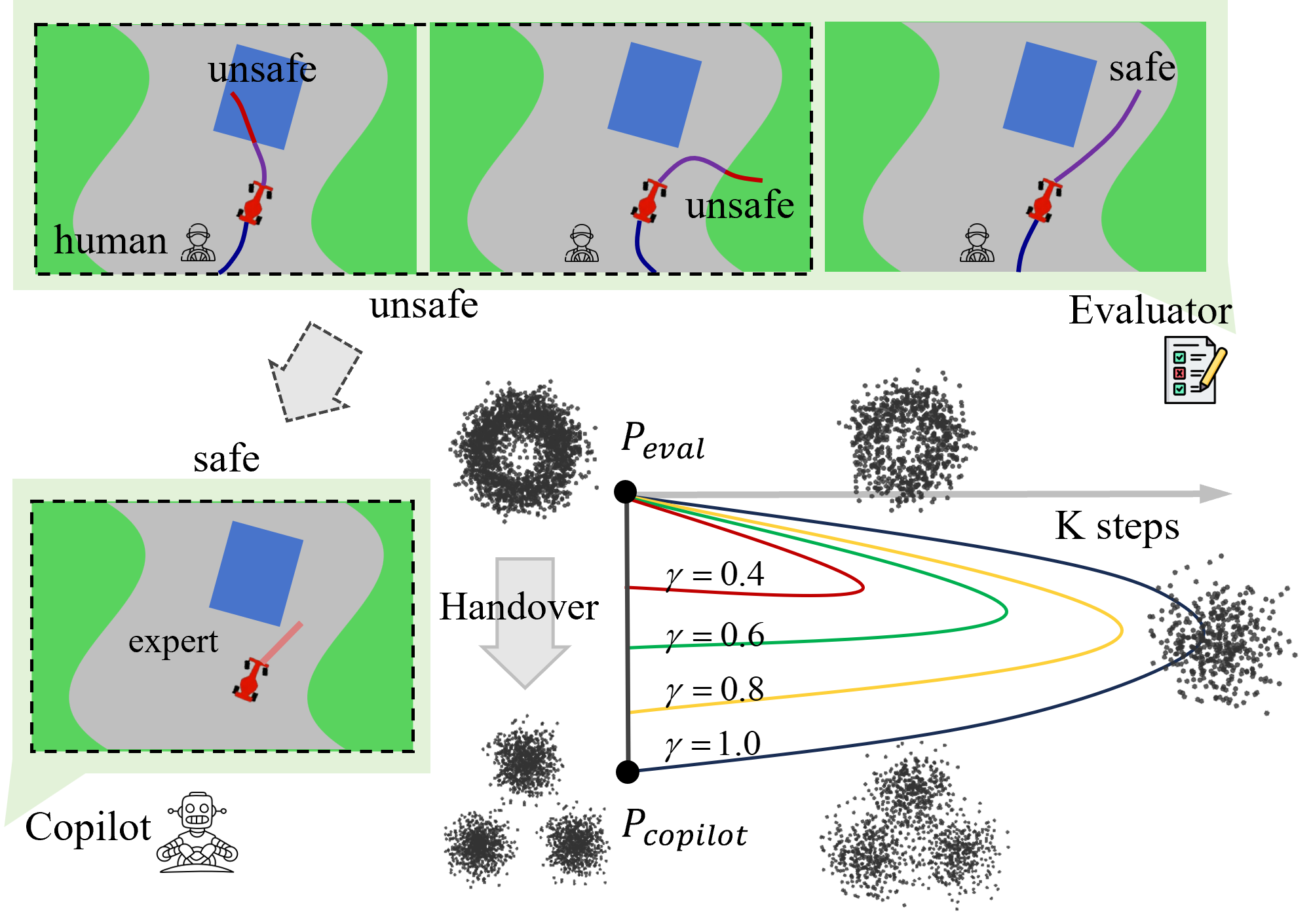
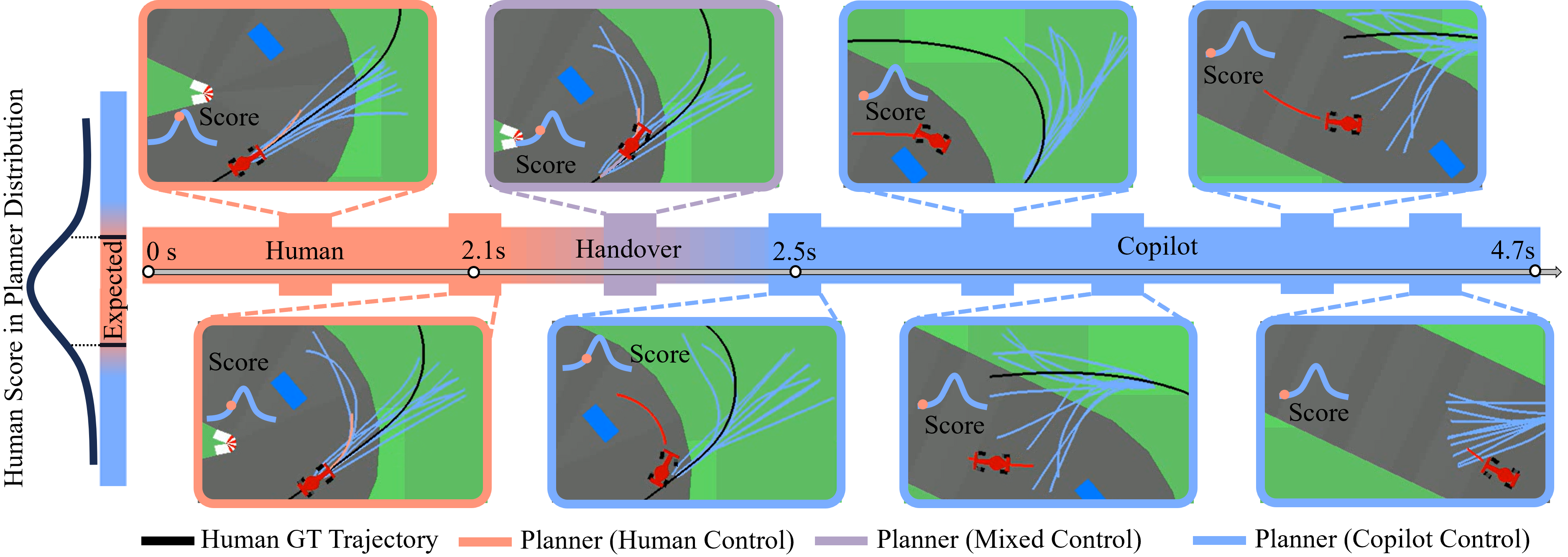
Contribution: We propose Diffusion-SAFE, a closed-loop shared autonomy framework with two diffusion policies (Fig. 1): the evaluator generates long-horizon multimodal action sequences aligned with human intent in real time, predicting potential risks in human driving; the copilot acts as a trajectory planner, mimicking expert drivers to provide optimal/suboptimal short-horizon action sequences. Moreover, in the control transfer process, we employ a modulation of the forward and reverse processes of the copilot diffusion model to transform potential unsafe human actions into safe actions sampled from the copilot. We also demonstrate that our framework works successfully both in simulation and on real ROS based race cars.
II Related Work
Shared autonomy has shown promising results—for example, AI-assisted control in the Lunar Lander game [5] and haptic-guided medical robotics [3]. Still, significant challenges remain, particularly in the AV domain.
Limitations in Prediction Horizon for Control Handover. Transitioning control in shared autonomy is critical but complex, with poorly timed handovers posing safety risks. Effective handover requires a system with a long prediction horizon to infer human intent. Current Driver Monitoring Systems (DMS), which depend on gaze, posture, and physiological signals [9], provide only momentary assessments and lack predictive capability, possibly leading to untimely or unnecessary transitions. Additionally, DMS relies on hand-tuned reward functions that can be brittle and case-sensitive.
Limitations in Multimodality Representation and OOD Handling. Human intent is inherently inconsistent and multimodal. To capture the underlying patterns of human intent and generate possible future trajectories, existing planners often rely on discrete top-k predictions [10]. However, this approach may fail to fully account for all or most potential driving intentions. Current trajectory planners often use recurrent models such as RNNs, LSTMs, or GRUs [11] to extract information from historical trajectories and the environment. However, these discriminative models struggle to model future uncertainties comprehensively.
Limitation in Continuous Feedback and Copilot Integration. Existing autonomous driving systems primarily focus on trajectory prediction for full autonomy or complete human operation in an offline inference manner, lacking the adaptability needed for real-time collaboration and control handover in shared autonomy [12].
To address these limitations, we propose a closed-loop shared autonomy system, Diffusion-SAFE, inspired by the success of diffusion policies in robotic manipulation [13]. Specifically, we leverage vision-conditioned diffusion models [14], which effectively capture multimodal distributions and integrate their forward and reverse processes to ensure a gradual transition of control authority. In particular, diffusion models generate trajectories as continuous probability distributions, making them well suited for complex multimodal scenarios, such as bypassing an obstacle from either the left or right [13]. Unlike discrete top-k predictions, they capture the full probabilistic distribution of trajectories [10]. Additionally, by leveraging stochastic sampling, diffusion models generate diverse and plausible trajectory predictions, naturally incorporating uncertainty about the future. Furthermore, diffusion models seamlessly integrate with real-time feedback by adjusting the forward step ratio. This enables progressive collaboration and smoother control transitions, making them well suited for dynamic shared autonomy applications [6].
III Method
III-A Problem Formulation
The goal of this work is to ensure safe driving performance and facilitate control transfer in collaborative human-robot driving through a closed-loop framework. This framework leverages two diffusion model-based policies:
Long-horizon policy as evaluator: It models multimodal action sequences aligned with human intent:
| (1) |
where it evaluates the similarity between predicted and actual human-driven trajectories.
Short-horizon policy as copilot: It models the conditional distribution of future expert action sequences:
| (2) |
supporting safe and efficient planning in human-in-the-loop scenarios.
To quantify human performance and determine the need for handover, we define a similarity score based on the negative log-likelihood (NLL):
| (3) |
The handover process is triggered when the similarity score exceeds a predefined threshold ; the progressively changing forward step ratio of the copilot diffusion model ensures that control is transferred seamlessly when human actions deviate significantly from safe or optimal trajectories.
III-B Approach Overview
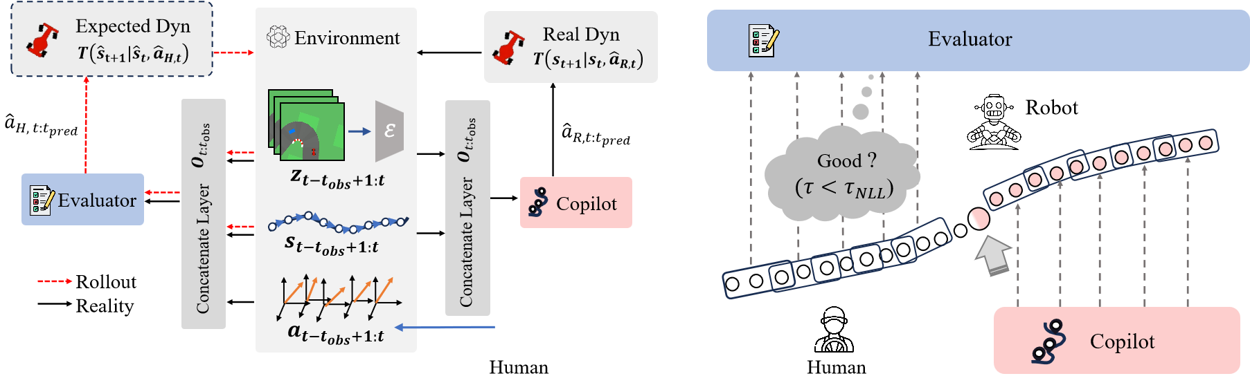
Our pipeline (shown in Fig 2) uses an evaluator model that takes as input a sequence of past states, actions, and visual context to predict the next action sequence aligned with human intent. We quantify human performance and decide if control handover is needed via a negative log-likelihood (NLL)–based score. Specifically, if a potential unsafe action is detected, we modulate the forward and reverse processes of the copilot diffusion model to transition from the evaluator’s output to a sample drawn from the copilot’s expert trajectories. Once control is transferred, the copilot takes the past states and visual context as input, then samples and rolls out an expert-level action sequence. In real-world implementations, the same pipeline applies, but includes an additional step for acquiring visual context (introduced in Section IV).
III-C Simulation Description and Setup
We conducted our simulated experiments in CarRacing-v0, a component of the OpenAI Gym framework [15], which was originally designed for reinforcement learning and provides a simple 2D simulation in which a single car navigates through a randomly generated track. We selected CarRacing-v0 for its simplicity, adaptability, and suitability to test our shared autonomy framework, as it requires real-time human interaction; moreover, unlike other environments that simplify vehicle dynamics using a unicycle model [16], CarRacing-v0 leverages the Box2D library [17], which supports more complex and nonlinear 2D physics simulations to enhance realism. The car model we use in our work comprises five bodies: a central hull and four wheels, connected through joint constraints, enabling more accurate modeling of physical interactions and vehicle dynamics. CarRacing-v0 offers a top-down racing simulation in which the track is randomly deformed into a circular shape for each lap. It also allows users to run and collect data via a keyboard or joystick controller (introduced in Section III-F). The actions in the simulation are executed via the built-in step function of the Box2D library, which takes an action vector as input and advances the system dynamics by a fixed time step of 0.1 seconds. The single action consists of three components:
-
•
Steering: A continuous action , where denotes a full left turn and a full right turn.
-
•
Acceleration: A throttle input , controlling the vehicle’s forward movement.
-
•
Brake: A braking input , where completely restricts wheel rotation.
III-D Construction of Conditioning Information
In our work, we use two diffusion model-based policies to realize the closed-loop framework. We use DDPM [14] to approximate the conditional distribution and . In this section, we will introduce the construction of conditioning information for these two policy models.
For the policies to take into account the surrounding environment, we capture the visual context of the environment by collecting 96×96 pixel RGB images. To reduce computational complexity, we employ a lightweight Autoencoder to translate these images into a lower-dimensional latent vector (model details are provided in the code). This approach helps streamline the diffusion process and reduce both inference time and computational cost [18].
The observation information of both models at time is denoted as , where and represent the state and latent variables respectively. Each state encapsulates the car’s pose and velocity. For simpler subscript notation, the observation information over steps is represented as a concatenated matrix . The predicted human action sequence over steps is represented as a concatenated matrix .
III-E Diffusion Pipeline for Action Sequence Prediction
In this section, we provide a brief overview of the conditional diffusion model in the context of action sequence prediction, and introduce its application to shared autonomy in our work, where diffusion is utilized as a partial control mechanism.
A diffusion model captures the probability distribution by inverting a forward diffusion process, which gradually adds Gaussian noise to the intermediate distribution of an initial sample . The amounts of added noise depend on a predefined variance schedule (here we choose the cosine schedule [6]). For reverse denoising process, a neural network takes the noisy input at time step and predicts the added noisy sample and the diffusion time step , and learns to predict the added noise . To generate a sample from the learned distribution, we start by drawing a sample from the prior distribution and iteratively denoise this sample times using :
| (4) |
where is Gaussian noise added back at each iteration. , , and are functions of the iteration step , also referred to as the noise schedule.
Moreover, diffusion models can be easily extended to model conditional distributions by adding an additional input to the denoising neural network . In our work, we leverage this property into the evaluator and copilot in the context of action sequence prediction. To capture conditional distributions and , we modify Eq. 4 to:
| (5) |
| (6) |
where and represent the denoising neural networks for the evaluator and the copilot policy, respectively. Notably, the evaluator conditions on both historical observations and actions (Eq. 5), whereas the copilot policy conditions only on historical observations (Eq. 6). To unify the notation for later use, we denote the conditioning information for both the evaluator and copilot models as .
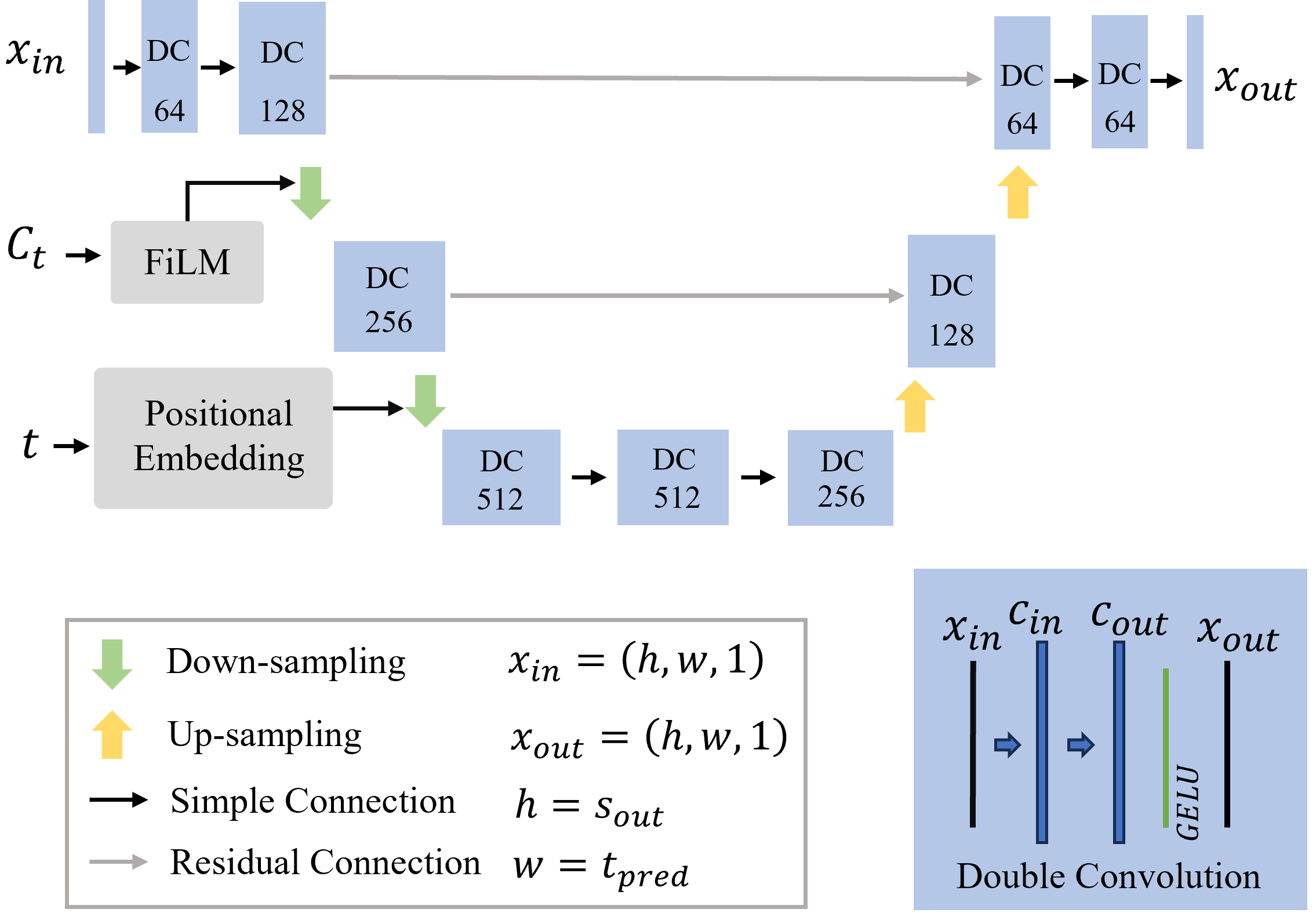
As depicted in Fig.3, our model architecture is influenced by the U-Net design with residual connections by Zagoruyko et al. [19]. Similar to the original diffusion implementations by Ho et al. [14], our architecture combines double convolution blocks (as detailed in Fig. 3) with up-sampling and down-sampling using pooling operations. These operations incorporate the conditioning information using the Feature-wise Linear Modulation (FiLM) layers [20] and the current time step after applying positional embedding.
The FiLM layers use conditioning information matrix to modulate the input features at each time step through dynamic scaling and shifting , defined as:
| (7) |
Here, and are trainable parameters derived from . This enables the diffusion model to adapt its feature representation dynamically based on past observations, ensuring that the generated trajectories align with the demonstrated behavior and environmental conditions.
Since diffusion models require explicit temporal information to represent the relative position of each time step in the denoising chain, we employ positional embedding, inspired by the transformer architecture [21]. Positional embedding explicitly encodes the time step as a unique feature, enabling the model to incorporate temporal dependencies more effectively. Specifically, we use a fixed sine-cosine embedding scheme for an embedding vector of dimension which is added to the input , providing explicit information about the current step in the denoising process. By integrating positional embeddings, the diffusion model ensures that the denoising function is aware of the sequential nature of the action generation process.
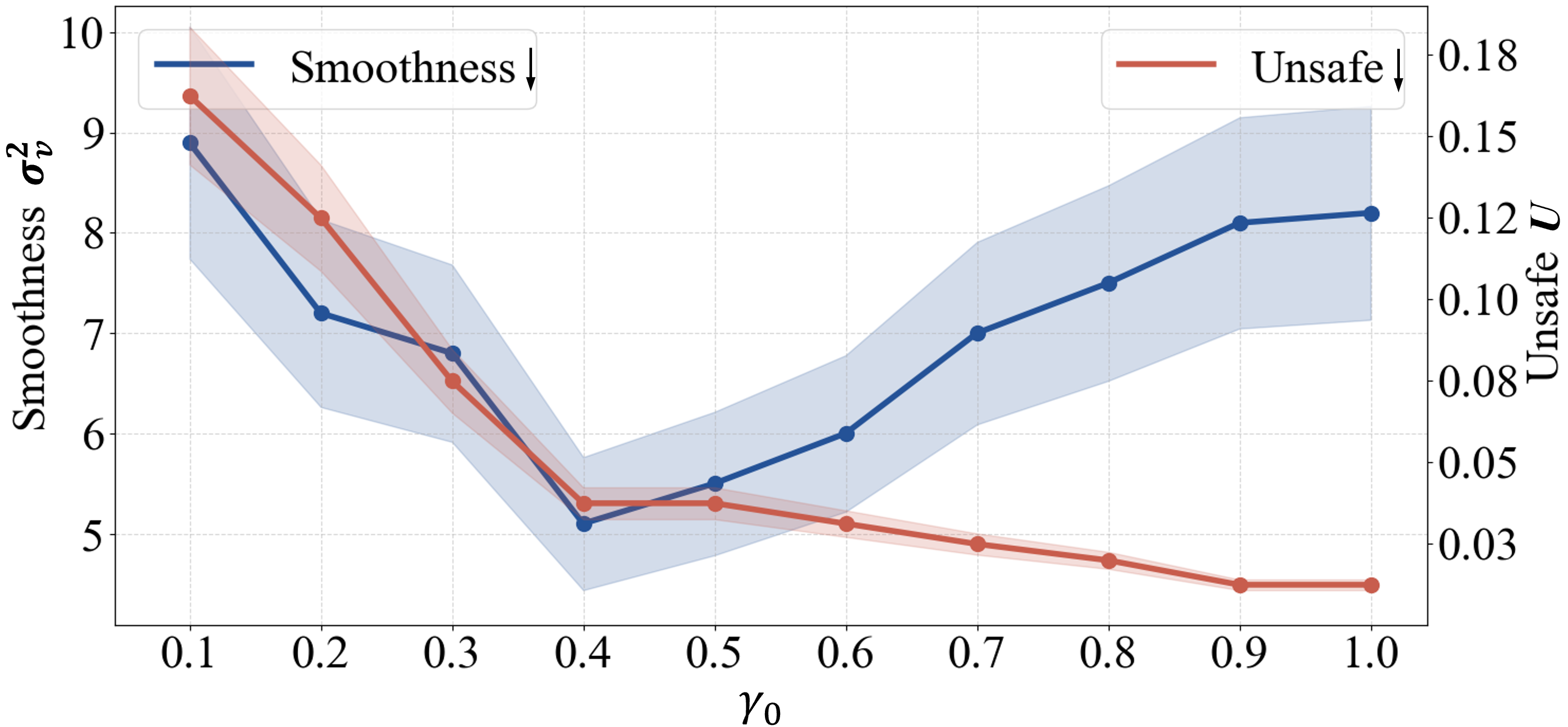
Inspired by the idea of shared autonomy as partial diffusion by Yoneda et al. [6], we modulate the forward and reverse diffusion processes in the copilot model to transform unsafe human actions into samples from the copilot expert distribution. In our work, Diffusion-SAFE leverages the concept of partial diffusion to achieve the handover process of control authority between the human and the copilot. Specifically, the forward diffusion process progressively corrupts the human distribution by introducing noise, while the reverse diffusion process refines the noisy samples to align with the safe copilot distribution (demonstrated in Fig 1). Here, we introduce the forward diffusion ratio , where is the forward steps in the inference stage of the copilot model. This ratio determines the number of forward diffusion steps applied to the human action . By changing , we can adjust the balance between preserving human input and following the safe behavior of the copilot: when is small, human intent is well preserved, and thus with limited alignment to ; in contrast, larger values would lead the system to prioritize aligning with the copilot policy over human input.
To progressively transition control from the human to the copilot, we dynamically modulate from to 1, where is the critical threshold determined empirically. To find the optimal , we evaluate the handover process based on smoothness and unsafe rate. Specifically, smoothness is measured by the variance of velocity, which quantifies the deviation of velocity from its mean over time:
| (8) |
where is the velocity at time step , is the mean velocity over the time period, is the total number of time steps. A lower variance indicates a more stable and smoother velocity profile. The unsafe rate is defined as the proportion of trials in which the vehicle goes off-road or collides with obstacles during the handover process:
| (9) |
where is the unsafe rate, is the number of trials where the vehicle goes off-road or collides with obstacles, is the total number of trials. By jointly considering smoothness and the unsafe rate , we select based on the performance analysis shown in Fig. 5.
III-F Dataset and Model Training Details
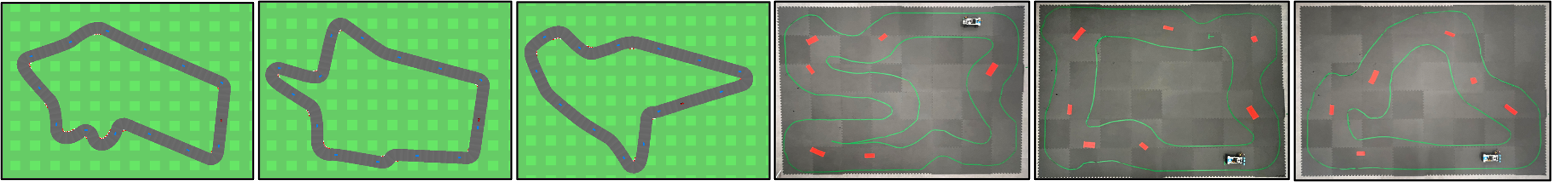
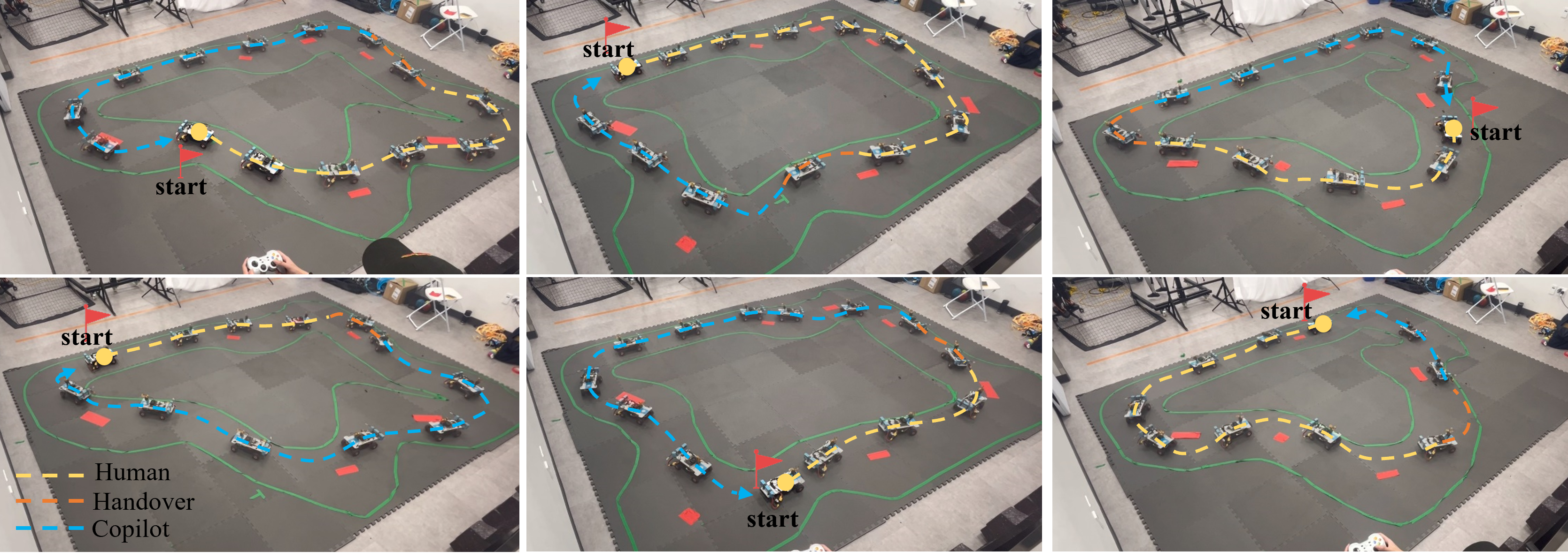
Based on the CarRacing-v0 environment introduced in Section III-C, we collected an expert driving dataset and a human driving dataset through demonstrations performed by different individuals using Xbox controllers. The Box2D physics engine generates a random closed-loop track for each lap, with variations in curvature and the number of turns upon every reset (shown in Fig. 4). Top-down RGB image sequences, joystick and trigger events (mapped to steering, throttle, and brake actions), and state sequences (including translation, orientation, and velocity) were recorded into Zarr files as human driving dataset. The expert driving dataset is recorded in a similar manner, but without the action component. The dataset serves as the foundation for training both the Autoencoder and the diffusion models.
We first train a lightweight Autoencoder to reconstruct input images by minimizing the MSE loss between the input RGB image and the reconstructed output. The encoder compresses the input into a latent vector , while the decoder reconstructs the original image using transposed convolutions. Once trained, only the encoder is used to extract the latent vector, which serves as the visual representation of the conditioning information and is subsequently utilized by the diffusion model. Note that Autoencoder is trained on the image component of the demonstration dataset.
The evaluator and copilot are trained on different dataset for different purposes. The evaluator policy is learned from ‘average human demonstrations’ dataset, denoted as , which include both typical and non-positive examples such as minor off-road incidents or collisions. We assume these demonstrations, while involving occasional deviations, follow discernible patterns and exclude erratic, nonsensical behaviors. This enables the evaluator to capture human intent and predict action sequences aligned with their behavioral patterns. In contrast, the copilot policy is trained exclusively on safe ‘expert demonstrations’, denoted as , comprising suboptimal and optimal examples. As a result, the evaluator focuses on learning and mimicking human behavior, including imperfections, while the copilot specializes in generating safe and reliable action sequences. This training approach ensures that both models fulfill distinct but synergistic roles.
Another key difference between the evaluator and copilot models lies in their observation and future horizons. The evaluator policy, designed to infer human intent from demonstrations, benefits from long-horizon predictions. In contrast, the copilot policy prioritizes short-horizon predictions to achieve faster and more stable action sequences, given the computational expense of diffusion models. Both models are trained by minimizing the evidence lower bound (ELBO) of the loss function at each time step. For both models, we conducted ablation studies on the observation and prediction horizon in Section V-B.
IV Real-World Experiments
IV-A Hardware Setup
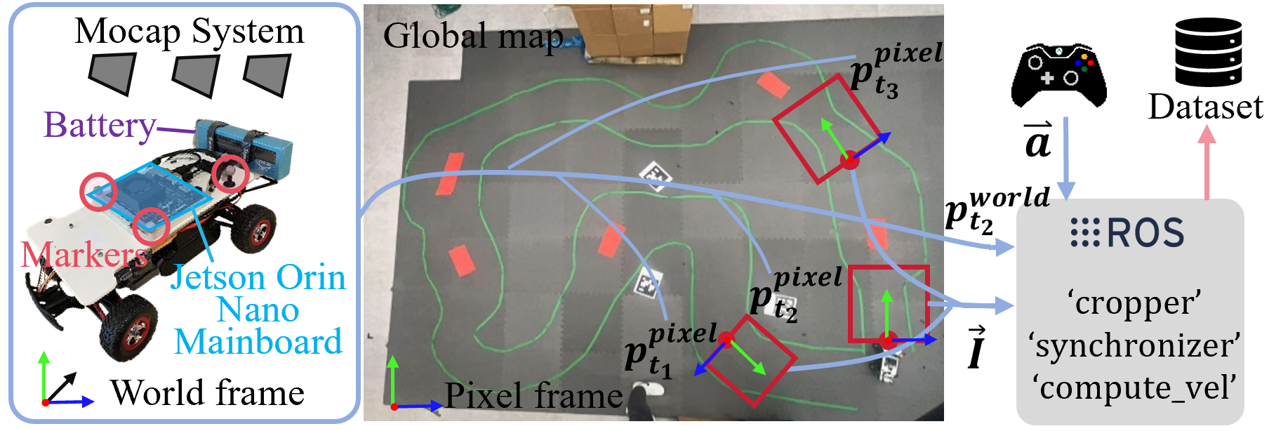
We conducted real-world experiments on a ROS-based race car equipped with a Jetson Orin Nano for onboard processing (shown in Fig. 7). A Windows11 computer (Intel Core i9-9900KS CPU, 64GB RAM) running Motive software streamed data from a 13-camera OptiTrack motion capture system. To localize the car in the world coordinate system, four motion capture markers were selected in Motive to define a rigid body representing the car. For data transmission and network communication, the Virtual-Reality Peripheral Network (VRPN) was used to link Motive and ROS. The VRPN server on the Motive host computer transmitted pose data (2D translation and 1D orientation) as network packets to the ROS client.
IV-B Real-World Data Collection
To simplify the setup and avoid mounting a physical camera on the car, we captured a single top-down photo of the entire track. Using pose data from the motion capture system, we cropped real-time image patches from the top-down photo to simulate the car’s perspective. The detailed pipeline is shown in Fig. 7.
We first printed four AprilTags[22] and placed them on the ground, each with a motion capture marker attached to one of its corners. Using the motion capture system, we obtained the positions of these markers in the world frame. Next, we used the AprilTag library to retrieve the pixel coordinates of the corners in the image. Finally, we used OpenCV’s getPerspectiveTransform function, which takes four corresponding points in the world frame (from the motion capture system) and the pixel frame (from the AprilTag detection) to compute the perspective matrix , which maps the world coordinates to the pixel coordinates. To create a top-down perspective similar to the simulation environment setup, we implemented a ROS node to crop image patches from the global photo as visual information in real time. The pose of the bounding box in the pixel frame is denoted as . Given the world coordinates from the motion capture system , the corresponding pixel coordinates can be computed as . During real-time deployment, the motion capture system streams the car’s position and orientation data, which we access via the VRPN client. Specifically, represents the bottom-center of the bounding box as Fig. 7 shown, with as the rotation angle used for cropping.
The frequency of the motion capture system is 100Hz while that of the control signals from joystick is 10Hz. To address the different frequencies of the motion capture system and the joystick controller, we implemented a ROS node to align the nearest corresponding actions from the controller with the poses from the motion capture system. Specifically, the node identifies the closest pose data from motion capture system and matches it with the corresponding action data from the joystick controller commands. The synchronized data are then packaged into a message and published on a ROS topic.
To collect real-world data and deploy the framework pipeline in a physical setting, we adopt the Zarr structure described in the CarRacing-v0 introduced in Section III-F. The car’s steering, throttle, and brake data are recorded as actions in the Zarr files, while synchronized image and pose data from the motion capture system are recorded as images and states respectively. Datasets are collected through demonstrations conducted by different individuals using Xbox controllers. In practice, we generated a variety of racing tracks (with combinations of different turns and obstacles) using green tape as track bounds and red tape as obstacles (illustrated in Fig. 4). Consistent with the simulation training logistics, the Autoencoder’s training dataset is derived from the image component of the demonstration dataset. Real-world examples are shown in Fig. 8.
V Evaluation
V-A Evaluation Metrics
To comprehensively evaluate the predicted trajectories, we introduce three metrics for the copilot diffusion model and the evaluator diffusion model, adapted from the nuPlan benchmark metrics [23]. These metrics are carefully designed to capture the multifaceted aspects of trajectory prediction.
V-A1 Human Driving Similarity
Human driving similarity quantifies how closely a maneuver predicted by the evaluator diffusion model aligns with human driving behavior. Adopted as widely used in the AV industry, measurements of the mean average displacement & orientation error over a set of predictions ( in our case), known as minADE-K and minAOE-K respectively, are used in our work to assess the prediction performance of the evaluator model. Both metrics evaluate the model’s ability to include the ground-truth human trajectory within its predicted distribution, making it particularly relevant for multimodal prediction models that aim to capture the variety in plausible outcomes. Lower minADE-K and minAOE-K indicate more desirable outcomes, reflecting the preference for trajectories that closely mimic human driving.
V-A2 F1 Score
The F1 score is the harmonic mean of precision and recall, measuring the accuracy and completeness of the model to detect unsafe conditions. It evaluates the performance of the copilot model in differentiating between positive (unsafe off-road) and negative (safe on-road) classes. We evaluated the copilot based on its predicted trajectories on 15 simulated and 15 real tracks with 10 trials per track.
V-A3 Safety
The safety score evaluates the prediction quality of the copilot model by incorporating both the collision rate and the off-road rate to assess collision-free performance. The collision rate quantifies the ratio of trajectories that collide with obstacles to the total number of sampled rollouts ; off-road rate measures the ratio of trajectories that go off-road to the total number of sampled rollouts . Lower collision and off-road rates indicate safer copilot predictions.
| (10) |
V-A4 Computation Time
Computation time refers to the computational duration needed for the model to generate predictions once it has received the input in a proceeding manner. We include the sampling time (in seconds) as a performance metric for both the evaluator and the copilot.
V-B Ablations
We perform an ablation study to evaluate the effectiveness of model components with results summarized in Table I and II, with the best model (‘ours’) demonstrated in the real world. These studies were performed on both the evaluator and the copilot model. Specifically, we analyzed the impact of position, visual context, and observation & prediction horizons on the performance of these models. In addition, we examined how the incorporation of the past human action sequence impacts the effectiveness of the evaluator model. The unit of horizon is the step (0.1s).
| Evaluator | Horizon Obs/Pred | minADE-K | minAOE-K (rad) | Compute (s) |
| Ours (default) | 20/30 | |||
| w/o position | 20/30 | |||
| w/o action | 20/30 | |||
| w/o visual context | 20/30 | |||
| Ablate Obs 1 | 15/30 | |||
| Ablate Obs 2 | 25/30 | |||
| Ablate Pred 1 | 20/25 | |||
| Ablate Pred 2 | 20/35 | |||
| Ours (Real-World) | 20/30 |
| Copilot | Horizon Obs/Pred | F1 | Collision | Off-Rd. | Compute (s) |
| Ours (default) | 10/15 | 0.98 | 0.02 | 0.01 | |
| w/o position | 10/15 | 0.52 | 0.21 | 0.16 | |
| w/o visual context | 10/15 | 0.48 | 0.53 | 0.43 | |
| Ablate Obs 1 | 5/15 | 0.88 | 0.06 | 0.03 | |
| Ablate Obs 2 | 15/15 | 0.95 | 0.03 | 0.01 | |
| Ablate Pred 1 | 10/10 | 0.98 | 0.02 | 0.01 | |
| Ablate Pred 2 | 10/20 | 0.91 | 0.10 | 0.07 | |
| Ours (Real-world) | 10/15 | 0.85 | 0.08 | 0.05 |
V-C Comparison with Baselines
We utilize the ability of the diffusion policy to inherently express multimodal distributions. Our method is compared to the following multimodal methods: LSTM-GMM [24] and Behavior Transformers models (BET) [25]. The results are summarized in Tables III and IV.
V-C1 LSTM-GMM
LSTM-GMM combines LSTM for temporal feature extraction with GMM to model continuous multimodal action distributions. Notice that we need to pre-define the number of clusters for GMM or k-means steps.
V-C2 BET
BET models employ transformers to model multimodal behaviors by learning from demonstrations. Note that this method also requires the predefined number of modes.
| Evaluator | minADE-K | minAOE-K (rad) | Computation (s) |
| Ours | |||
| LSTM-GMM | |||
| BET |
| Copilot | F1 | Collision | Off-Road | Computation (s) |
| Ours | 0.98 | 0.02 | 0.01 | |
| LSTM-GMM | 0.65 | 0.11 | 0.12 | |
| BET | 0.74 | 0.13 | 0.14 |
V-D Comparison with Simple Blending in Handover Process
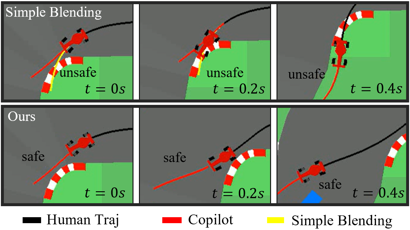
To evaluate our partial diffusion method in the handover process, we compare it to a simple blending method:
| (11) |
where is the blended action, is the blending coefficient which decreases over time to gradually shift control from human to the copilot, is the action of human, and is the action of the copilot. Fig. 9 shows that the simple blending method leads to unsafe off-road states, while our method safely completes the handover process. Notice that even after the simple blending method leads the vehicle to unsafe states, the copilot is able to correct it back to the track.
VI Conclusions
This work proposes a closed-loop framework, Diffusion-SAFE, capable of infering the driver’s intent, sampling safe trajectories, and dynamically adjusting the control authority from human to the autonomous system. Unlike traditional methods, our framework avoids making explicit assumptions about the high-level behaviors or intended goals of the drivers. It also facilitates smooth and gradual transitions of control from human drivers to the copilot model when future actions indicate potential safety risks. Moreover, our method eliminates the need for manually designing score functions to evaluate human driving performance and enables autonomous driving with multimodal strategies. Framework effectiveness is validated through simulations and select real-world experiments using ROS-based race cars, demonstrating its practical applicability and robust performance. Future work will focus on improving the computation speed by incorporating DDIM [26] or hybrid DDIM-DDPM methods.
References
- [1] D. A. Abbink, T. Carlson, M. Mulder, J. C. De Winter, F. Aminravan, T. L. Gibo, and E. R. Boer, “A topology of shared control systems—finding common ground in diversity,” IEEE Transactions on Human-Machine Systems, vol. 48, no. 5, pp. 509–525, 2018.
- [2] M. Marcano, S. Díaz, J. Pérez, and E. Irigoyen, “A review of shared control for automated vehicles: Theory and applications,” IEEE Robotics and Automation Letters, vol. 50, no. 6, pp. 475–491, 2020.
- [3] L. Xiong, C. B. Chng, C. K. Chui, P. Yu, and Y. Li, “Shared control of a medical robot with haptic guidance,” International Journal of Computer Assisted Radiology and Surgery, vol. 12, pp. 137–147, 2017.
- [4] P. Aigner and B. McCarragher, “Human integration into robot control utilising potential fields,” in Proceedings of International Conference on Robotics and Automation, vol. 1. IEEE, 1997, pp. 291–296.
- [5] S. Reddy, A. D. Dragan, and S. Levine, “Shared autonomy via deep reinforcement learning,” arXiv preprint arXiv:1802.01744, 2018.
- [6] T. Yoneda, L. Sun, B. Stadie, M. Walter, et al., “To the noise and back: Diffusion for shared autonomy,” arXiv preprint arXiv:2302.12244, 2023.
- [7] K. Vellenga, H. J. Steinhauer, A. Karlsson, G. Falkman, A. Rhodin, and A. C. Koppisetty, “Driver intention recognition: State-of-the-art review,” IEEE Open Journal of Intelligent Transportation Systems, vol. 3, pp. 602–616, 2022.
- [8] M. Flad, J. Otten, S. Schwab, and S. Hohmann, “Steering driver assistance system: A systematic cooperative shared control design approach,” in 2014 IEEE International Conference on Systems, Man, and Cybernetics (SMC). IEEE, 2014, pp. 3585–3592.
- [9] E. Shi, T. M. Gasser, A. Seeck, and R. Auerswald, “The principles of operation framework: A comprehensive classification concept for automated driving functions,” SAE International Journal of Connected and Automated Vehicles, vol. 3, no. 12-03-01-0003, pp. 27–37, 2020.
- [10] D. Wang, C. Devin, Q.-Z. Cai, F. Yu, and T. Darrell, “Deep object-centric policies for autonomous driving,” in 2019 International Conference on Robotics and Automation (ICRA). IEEE, 2019, pp. 8853–8859.
- [11] C. Tang and R. R. Salakhutdinov, “Multiple futures prediction,” Advances in neural information processing systems, vol. 32, 2019.
- [12] M. Marcano, S. Díaz, J. Pérez, and E. Irigoyen, “A review of shared control for automated vehicles: Theory and applications,” IEEE Transactions on Human-Machine Systems, vol. 50, no. 6, pp. 475–491, 2020.
- [13] C. Chi, Z. Xu, S. Feng, E. Cousineau, Y. Du, B. Burchfiel, R. Tedrake, and S. Song, “Diffusion policy: Visuomotor policy learning via action diffusion,” The International Journal of Robotics Research, p. 02783649241273668, 2023.
- [14] J. Ho, A. Jain, and P. Abbeel, “Denoising diffusion probabilistic models,” Advances in neural information processing systems, vol. 33, pp. 6840–6851, 2020.
- [15] G. Brockman, “Openai gym,” arXiv preprint arXiv:1606.01540, 2016.
- [16] N. Correll, B. Hayes, C. Heckman, and A. Roncone, Introduction to autonomous robots: mechanisms, sensors, actuators, and algorithms. Mit Press, 2022.
- [17] E. Catto, “box2d,” https://github.com/erincatto/box2d, 2023, accessed: 2023.
- [18] R. Rombach, A. Blattmann, D. Lorenz, P. Esser, and B. Ommer, “High-resolution image synthesis with latent diffusion models,” Proceedings of the IEEE/CVF Conference on Computer Vision and Pattern Recognition (CVPR), pp. 10 684–10 695, 2022.
- [19] S. Zagoruyko, “Wide residual networks,” arXiv preprint arXiv:1605.07146, 2016.
- [20] E. Perez, F. Strub, H. D. Vries, V. Dumoulin, and A. Courville, “Film: Visual reasoning with a general conditioning layer,” Proceedings of the AAAI Conference on Artificial Intelligence, vol. 32, no. 1, 2018.
- [21] A. Vaswani, “Attention is all you need,” Advances in Neural Information Processing Systems, 2017.
- [22] E. Olson, “Apriltag: A robust and flexible visual fiducial system,” IEEE Robotics and Automation Letters, pp. 3400–3407, 2011.
- [23] H. Caesar, J. Kabzan, K. S. Tan, W. K. Fong, E. Wolff, A. Lang, L. Fletcher, O. Beijbom, and S. Omari, “nuplan: A closed-loop ml-based planning benchmark for autonomous vehicles,” arXiv preprint arXiv:2106.11810, 2021, accessed: January 5, 2025. [Online]. Available: https://arxiv.org/abs/2106.11810
- [24] A. Mandlekar, D. Xu, J. Wong, S. Nasiriany, C. Wang, R. Kulkarni, L. Fei-Fei, S. Savarese, Y. Zhu, and R. Martín-Martín, “What matters in learning from offline human demonstrations for robot manipulation,” IEEE Robotics and Automation Letters, vol. 6, no. 4, pp. 6522–6529, 2021.
- [25] N. M. Shafiullah, Z. Cui, A. A. Altanzaya, and L. Pinto, “Behavior transformers: Cloning modes with one stone,” IEEE Robotics and Automation Letters, vol. 7, no. 4, pp. 10 456–10 463, 2022.
- [26] J. Song, C. Meng, and S. Ermon, “Denoising diffusion implicit models,” arXiv preprint, 2020, arXiv:2010.02502.