Digital Nets and Sequences for Quasi-Monte Carlo Methods
Abstract
Quasi-Monte Carlo methods are a way of improving the efficiency of Monte Carlo methods. Digital nets and sequences are one of the low discrepancy point sets used in quasi-Monte Carlo methods. This thesis presents the three new results pertaining to digital nets and sequences: implementing randomized digital nets, finding the distribution of the discrepancy of scrambled digital nets, and obtaining better quality of digital nets through evolutionary computation. Finally, applications of scrambled and non-scrambled digital nets are provided.
\nauthor
A thesis submitted in partial fulfillment of the requirements
for the degree of
Doctor of Philosophy
May 2002
Hong Kong Baptist University
Chapter 1 Introduction
We consider the problem of approximating , the integral of a function over the -dimensional unit cube :
Computing such a multidimensional integral is important since it has wide applications in finance [CM96, PT96], physics and engineering [Kei96, PT97] and statistics [Fan80, Gen92, Gen93]. Numerical integration methods, such as tensor product Newton Cotes and Gaussian quadrature, become impractical as increases since the error of the such methods converges like where is the smoothness of function.
Monte Carlo methods are often a popular choice to estimate such integrals. They use the sample mean of the integrand evaluated on a set, , with randomly selected independent points drawn from a uniform distribution on
Unfortunately the convergence rate of the quadrature error for Monte Carlo methods, , is relatively low.
To overcome the lower convergence rate of Monte Carlo methods, quasirandom sequences have been introduced. The basic quasirandom sequences replace a random set by a carefully chosen deterministic set that is more uniformly distributed on , and it often yields a convergence rate of . The quadrature methods based on low discrepancy sets are called quasi-Monte Carlo methods [Nie92, Tez95, HL98, Fox99].
This chapter introduces the basic definitions of quasi-Monte Carlo methods and the outline of the remaining thesis.
1.1 Quasi-Monte Carlo Methods
The most important property of quasirandom sequences is an equidistribution property. The quality of such uniformity for quasirandom sequences is measured by the discrepancy, which is a distance between the continuous uniform distribution on and the empirical distribution of the for . First we define the empirical distribution of the sequence as
| (1.1) |
where is the indicator function of the set . We define the uniform distribution on as
| (1.2) |
The discrepancy arises from the worst case error analysis of quasi-Monte Carlo quadratures. The Koskma-Hlawka inequality, which provides an important theoretical justification for the quasi-Monte Carlo quadratures, uses the discrepancy to provide an upper bound quadrature error of quasi-Monte Carlo methods:
| (1.3) |
where is said to have bounded variation in the sense of Hardy and Krause. If , then . For further understanding of see Niederreiter [Nie92]. indicates the star discrepancy which will be defined next.
The star discrepancy is the most widely studied discrepancy and it is defined as follows:
| (1.4) |
The star discrepancy can be thought as a special case of -star discrepancy which is defined by
| (1.5) |
Another discrepancy, which will be used in this thesis, given by [Hic96], called a generalized -discrepancy, is
| (1.6) |
where the notation means the fractional part of a number. The positive integer indicates the degree of smoothness of integrands in the underlying Hilbert space, and the parameter measures the relative importance given to the uniformity of the points in low dimensional projections of the unit cube versus high dimensional projections of the unit cube. The reproducing kernel leading to this discrepancy is for a Hilbert space of integrands whose partial derivatives up to order in each coordinate direction are square integrable [HH99]. It is known that the root mean square discrepancy for scrambled -nets decays as as [HH99, HY01] for . is the th Bernoulli polynomial (see [AS64]). The first few Bernoulli polynomials, which are used in this thesis, are and
See [Hic96] for further discussion about the -star discrepancy and several other discrepancies.
1.2 Integration Lattices
Rank-1 lattices, also known as good lattice point (glp) sets, were introduced by Korobov[Kor59] and have been widely studied since then. See [SJ94, Nie92] for further details. The formula for the node points of a rank-1 lattice is simply
| (1.7) |
where is the number of points, is an -dimensional generating vector of integers The formula for a lattice is rather simple. However finding a good generating vector that makes the lattice have low discrepancy for the chosen and is not trivial. Recently the formula for lattice is extended to an infinite sequence [HHLL01]. This is done by using the radical inverse function, . For any integer , let any non-negative integer be represented in base as , where the digits take on values between and . The function flips the digits about the decimal point, i.e.,
| (1.8) |
The sequence is called the van der Corput sequence. An infinite sequence of imbedded lattices is defined by replacing by , i.e.,
| (1.9) |
where the first points of this sequence are a lattice whenever is a power of [HHLL01].
1.3 Digital nets and Sequences
Let denote a prime number. For any non-negative integer , we define the vector as the vector of its digits, i.e., . For any point , let denote the vector of the digits of . Let denote predetermined generator matrices. The digital sequence in base is , where each is defined by
| (1.10) |
Here all arithmetic operations take place in mod . Thus, the right side of (1.10) should not give a vector ending in an infinite trail of s.
Digital nets and sequences are the special cases of -nets and -sequences and further explanation is given in Chapter 4.
1.4 -Nets and -Sequences
The concept of in -nets and -sequences provides one way to measure the quality of low discrepancy sequences. See [Nie92] for more detail explanations. Here we provide a brief outline of elementary intervals of -nets and -sequences.
Let and be integers. An elementary interval in base is a subinterval of of the form
with integer , . Such an elementary interval has volume .
Let be an integer. A finite set of points from is a -net in base if every elementary interval in base with the volume contains exactly points of a set, where is a nonnegative integer. Smaller values imply a better equidistribution property for the net. Obviously the best case is when , that is every -ary box of volume contains exactly one of the points of the set.
For a given , an infinite sequence of points from is a sequence in base if for all integers and the finite sequence is a -net in base .
The constructions of -nets and -sequences in base were introduced by Sobol’ [Sob67]. Later Faure [Fau82] provided -nets and -sequences for prime bases . The general definitions are given by Niederreiter [Nie87]. Mullen, Mahalanabis and Niederreiter [Nie95] provide tables of attainable -values for nets.
The advantage of using nets taken from -sequences is that one can increase through a sequence of values , , and all the points used in are also used in . Owen [Owe97a] introduces the -nets to describe such sequences.
The initial points of a -sequence are well distributed. For integers with , , and , a sequence of points is called a -net in base if every -ary box of volume contains points of the sequence and no -ary box of volume contains more than points of the sequence.
For functions of bounded variation in the sense of Hardy and Krause, the numerical integration by averaging over the points of a -net has an error of order . Niederreiter [Nie92] discusses more precise error bounds for -nets and -sequences.
1.5 Randomized Quasi-Monte Carlo Methods
Quasi-Monte Carlo methods can obtain a better convergence rate than Monte Carlo methods, because the points are chosen to be more uniform. However deterministic quasi-Monte Carlo methods have disadvantages compared with Monte Carlo methods. First, quasi-Monte Carlo methods are statistically biased since the points are chosen in certain deterministic way. Therefore the mean of the quadrature estimate is not the desired integral. Second, quasi-Monte Carlo methods do not facilitate simple error estimates while Monte Carlo methods provide straightforward probabilistic error estimates.
Randomizing quasi-Monte Carlo point is one way to overcome such disadvantages while still preserving their higher convergence rates. One may think of randomized quasi-Monte Carlo as a sophisticated variance reduction technique. There are two types of randomization. One is adding the same -dimensional random shift to every point. Let be the original low discrepancy point set, then , where is a random vector uniformly distributed on . This type of randomization, which was introduced in [CP76], is often used with lattice rule because shifted lattice rules retain their lattice structure. However, shifted nets do not necessarily remain as nets. Another type of randomization, which was proposed by Art Owen [Owe95], is a more sophisticated method that randomly permutes the digits of each point. And it often applies to nets because scrambled nets retain their nets properties. However, scrambled lattice rules do not necessary remain lattice rules. The more detail discussions on Owen’s scrambling can be found in Chapter 2.
1.6 Outline of the Thesis
In this chapter we have introduced the necessary background of quasi-Monte Carlo methods.
Chapter 2 discusses the randomization of the quasi-Monte Carlo methods specifically randomizing digital nets. Detailed descriptions of Owen’s randomization (or scrambling) and Faure-Tezuka’s randomization (or tumbling) are provided. The actual implementation of randomization for digital -sequences and some numerical results are presented.
Chapter 3 explores the distribution of the discrepancy of scrambled digital -nets which is based on recent theory. We fit the empirical distribution by a sum of chi squared random variables. The distribution of the discrepancy of randomized lattice points is presented also.
Finding better digital nets is the main content of Chapter 4. Here we use optimization methods to find the generator matrices for digital -nets. Evolutionary computation is introduced as a tool for a finding better net.
Chapter 5 presents the applications of the sequences that we have generated. Various problems are explored and the performance of the new sequences is compared with other existing low discrepancy sequences.
Finally the thesis ends with some concluding remarks.
Chapter 2 Implementing Randomized Digital -Sequences
This chapter introduces randomized digital -sequences. Section 2.1 explains the details of Owen-scrambling and Section 2.2 introduces Faure-Tezuka-tumbling. Section 2.3 mainly deals with our method of scrambling that is nearly as general as Owen’s scrambling and the detailed explanation of the implementation. Section 2.4 explains our efforts to improve the efficiency of the generation time of the scrambled and non-scrambled sequences and discusses the time and the complexity of our algorithm. Section 5 presents various numerical results on the discrepancy for the newly generated randomized -sequences.
2.1 Owen’s Scrambling
Owen [Owe95, Owe97a, Owe97b, Owe98, Owe99] proposes scrambled -sequences as a hybrid of Monte Carlo and quasi-Monte Carlo methods. This clever randomizations of quasi-Monte Carlo methods can combine the best of both by yielding higher accuracy with practical error estimates. The following is a detailed description of Owen’s scrambling.
Let denote the randomly scrambled sequence proposed by Owen. Let denote the digit of the component of , and similarly for . Then
where the are random permutations of the elements in mod chosen uniformly and mutually independently. Owen [Owe98] provides a geometrical description to help visualize his scrambling as follows: The rule for choosing is like cutting the unit cube into equal parts along the axis and then reassembling these parts in random order to reform the cube. The rule for choosing is like cutting the unit cube into equal parts along the axis, taking them as groups of consecutive parts, and reassembling the parts within each groups in random order. The rule for involves cutting the cube into equal parts along the axis, forming groups of equal parts, and reassembling the parts within each group in random order.
Owen [Owe95, Owe97b] states that a randomized net inherits certain equidistribution properties of -nets by proving the following propositions:
Proposition 1 If is a -net in base then is a -net in base with probability 1.
Proposition 2 Let be a point in and let be the scrambled version of as described above. Then has the uniform distribution on .
2.2 Faure-Tezuka’s Tumbling
Faure and Tezuka [FT00] proposed another type of randomizing digital nets and sequences. However the effect of the Faure-Tezuka-randomization can be thought as re-ordering the original sequence, rather than permuting its digits like the Owen-scrambling. Thus we refer to this method as Faure-Tezuka-tumbling as suggested by Art Owen (personal communication). The following describes details of Faure-Tezuka-tumbling.
For any , let . Then takes all possible values in its top rows. By the same token takes on all possible values in its top rows, but not necessarily in the same order. Therefore, the Faure-Tezuka-tumbled -net, , obtained by replacing of (1.10) by is just the same set as the original -net, , given by (1.10) for some .
2.3 Implementation
There is a cost in scrambling -sequences. The manipulation of each digit of each point requires more time than for an unscrambled sequence. In addition Owen’s scrambling can be rather tedious because of the bookkeeping required to store the many permutations. Here we present an alternative method that is only slightly less general than Owen’s proposal but is an efficient method of scrambling that minimizes this cost. This is called an Owen-scrambling to recognize that it is done in the spirit of Owen’s original proposal.
2.3.1 The Method of Scrambling
Let , be nonsingular lower triangular matrices and let be an vector. Assume that for all any linear combination of columns of plus does not end in an infinite trail of s. A particular Owen-scrambling of a digital sequence is defined as
| (2.1) |
The left multiplication of each generator matrix by a nonsingular lower triangular matrix yields a new generator matrix that satisfies the same condition (4.1) as the original. The addition of an just acts as a digital shift and also does not alter the -value. Therefore the scrambled sequence is also a digital -sequence.
To get a randomly scrambled sequence one chooses the elements of the and randomly. The resulting randomized sequence has properties listed in the theorem below. Although these properties are not equivalent to the Owen’s original randomization, they are sufficient for the analysis of scrambled net quadrature rules given in [Owe95, Hic96, Owe97a, Owe97b, Owe98, HH99, Yue99, YM99, HY01].
Theorem 1
Let be an Owen-scrambling of a digital -sequence where elements of are all chosen randomly and independently. The diagonal elements of are chosen uniformly on , and the other elements are chosen uniformly on . Then this randomly scrambled sequence satisfies the following properties almost surely:
-
i.
is uniformly distributed on ;
-
ii.
if for and , then
-
a.
for
-
b.
are uniformly distributed on ;
-
c.
are independent for
-
a.
-
iii.
is independent from for
Proof The qualification “almost surely” is required to rule out the zero probability event that for some there exists a linear combination of columns of plus that ends in an infinite trail of s. Assertion iii. follows from the fact that the elements of , and are chosen independently of each other. Now the other two assertions are proved.
Note from (2.1) that , where is the row of , and all arithmetic operations are assumed to take place in the finite field. Since is distributed uniformly on , it follows that is also distributed uniformly on .
To prove ii. consider . Under the assumption of ii. the first rows of are zero, which implies that the first rows of are also zero, since is lower triangular. This immediately implies iia. Furthermore, , where is the diagonal element of . Since , and is a random nonzero element of , it follows that is a random nonzero element of . Combined with i., this implies iib. For it follows that . The fact that , and is uniformly distributed on , combined with i. now imply iic.
To understand why the randomization given by (2.1) is not as rich as that originally prescribed by Owen, consider randomizing , the first digit of for different values of . The take on different values, and there are possible permutations of these values. However, the formula given by (2.1) is , where denotes the element of , and denotes the element of . Since there are only possible values for and only possible values for , this formula cannot give at most permutations.
The Faure-Tezuka-tumbling [FT00] randomizes the digits of before multiplying by the generator matrices. Let , be a nonsingular lower triangular matrix, and let be an vector with a finite number of nonzero elements. A particular tumbling, , of a digital sequence is defined as
| (2.2) |
A particular scrambling-tumbling, , of a digital sequence is defined as
| (2.3) |
in order to obtain random Faure-Tezuka-tumbling the elements of and are chosen randomly.
The scrambling method described here applies only to digital -sequences. Since all known general constructions of -nets and -sequences are digital constructions [Sob67, Fau82, Nie88, Lar98a, Lar98b, NX98], this restriction is not serious. The algorithm we implement here builds on the algorithms of [BF88, BFN92] and includes the recent digital Niederreiter-Xing sequences by [NX96, NX98].
2.3.2 Generators for the Randomized Nets
Generators for scrambled Sobol’ [Sob67], Faure [Fau82], and Niederreiter [Nie88] points have been programmed following the Fortran codes of [BF88, BFN92]. Below the differences and improvements that we have made are highlighted and explained. The code for the Niederreiter points has been extended to higher dimension by Giray Ökten, and we have employed this extension. A generator for Niederreiter-Xing points has been coded based on the generator matrices provided by [Pir02].
The different scrambled or non-scrambled sequences given by (1.10), (2.1), and (2.2) are just special cases of (2.3). Thus, (2.3) is the basic algorithm to be implemented, with different choices given to the user as to how to choose the matrices and the vectors .
In practice one cannot store all the entries of an matrix. Assuming that is the maximum amount of points that is required in one run, and that is the number of digits to be scrambled. Then, one can restrict to matrices, to matrices, to vectors, and to a vector. One might think that it is best to scramble all available digits, but Section 2.4 provides evidence that this is not necessary.
The value of , the maximum possible value of , is 31, which corresponds to the number of bits in the largest integer available. When , the algorithms for generating digital sequences may be implemented more efficiently by storing an array of bits as an integer. For the scrambled Sobol’ generator the value of , the maximum dimension is , the same as in [BF88]. For the scrambled Faure sequence, , and for the scrambled Niederreiter generator . For the Niederreiter-Xing points based on the generator matrices available so far. The program may be modified to allow for higher dimensions as the generator matrices become available.
Another time saving feature is to use a gray code [Lic98]. Recursively define the vector function as follows:
is the Kronecker delta function, and where again all arithmetic operations take place in the finite field. For example, if , then
Note that only one digit of changes as the argument is increased by one. Replacing by in (2.4) still results in a scrambled digital sequence; it just has the effect of re-ordering the points. The efficiency advantage is that the digits of the point can be obtained from those of the point by the iteration:
| (2.5) |
where is the column of .
The implementations of the scrambled Sobol’ and Niederreiter sequences closely followed the structures of the original program and our changes were rather minor. However, the structure of the Faure sequence generator has been altered more substantially to improve efficiency. The scrambled Sobol’, Niederreiter, and Niederreiter-Xing generators all have base , which allows the use of logical operations instead of additions and multiplications.
2.3.3 Time and Space complexity
This section considers the number of operations and the amount of memory required to generate the first points of a scrambled )-sequence with . The space required to store the scrambled generator matrices is , where is the number of digits scrambled. The time required to generate and pre-multiply the matrices is . To generate one new point from the scrambled sequence requires just operations according to (2.5), so the total number of operations to generate all points is . Thus, the preparations steps take proportionally negligible time as . Note that for unscrambled points the corresponding time and space complexities can be obtained by replacing by .
The following table shows time comparison of sequence generating time of unscrambled and scrambled digital point sets using . The times have been normalized so that the time to generate the Sobol’ set equals 1.
| Algorithm | SOBOL | SSOBOL | NIED | SNIED | Old FAURE | FAURE | SFAURE |
|---|---|---|---|---|---|---|---|
| Time | 1 | 2 | 2 | 2 | 10 | 3 | 6 |
From the table it shows that generating time for scrambled Sobol’, Niederreiter and Faure sequences are about 2 times more than that of the original sequences based on the same number of extra digit scrambling. This is due the fact that one must manipulate digits of each number, not just . The new Faure generator takes about the time of the original one due to the use of the gray code.
2.4 Numerical Results
The discrepancy used in here is the squared discrepancy (1.1) and it has been scaled by a dimension-dependent constant so that the root mean square scaled discrepancy of a simple random sample is .
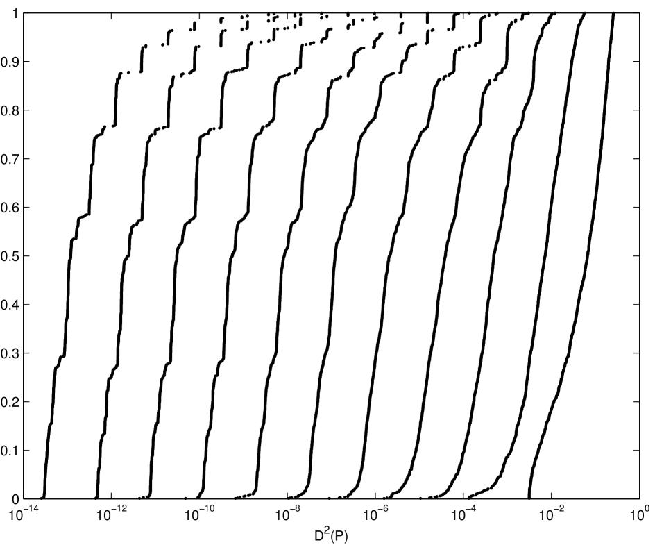
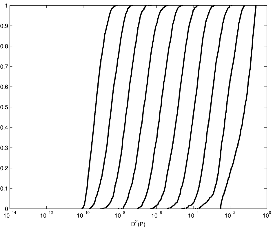
Figures 2.2 shows the histogram of the distribution of the square discrepancy of the particular Owen-scrambled Sobol’ sequence for the different numbers of scrambled digits, . has been chosen to be , , and for and with 200 independent replications. The range of the -axis is are in this figure. From the figure, there is only little distinction in the distribution of the square discrepancy for and . However a larger number of scrambled digits produces a wider range of discrepancies. From Figure 2.3 the root mean square discrepancies for and are nearly the same. However the root mean square discrepancy for looses the benefit from scrambling as increases.
Figures 2.3 and 2.4 plot the discrepancy of the particular Owen-scrambled Sobol’ sequence for different choices of and the choices are same as before. The choices of dimension are and . These figures show the root mean square discrepancy of 100 different replications. There is almost no difference in the root mean square discrepancy between scrambling or digits. However for the discrepancy looses its superior performance as increases, which indicates an insufficient number of scrambled digits. Also notice that choosing the number of scrambled digits is independent from .
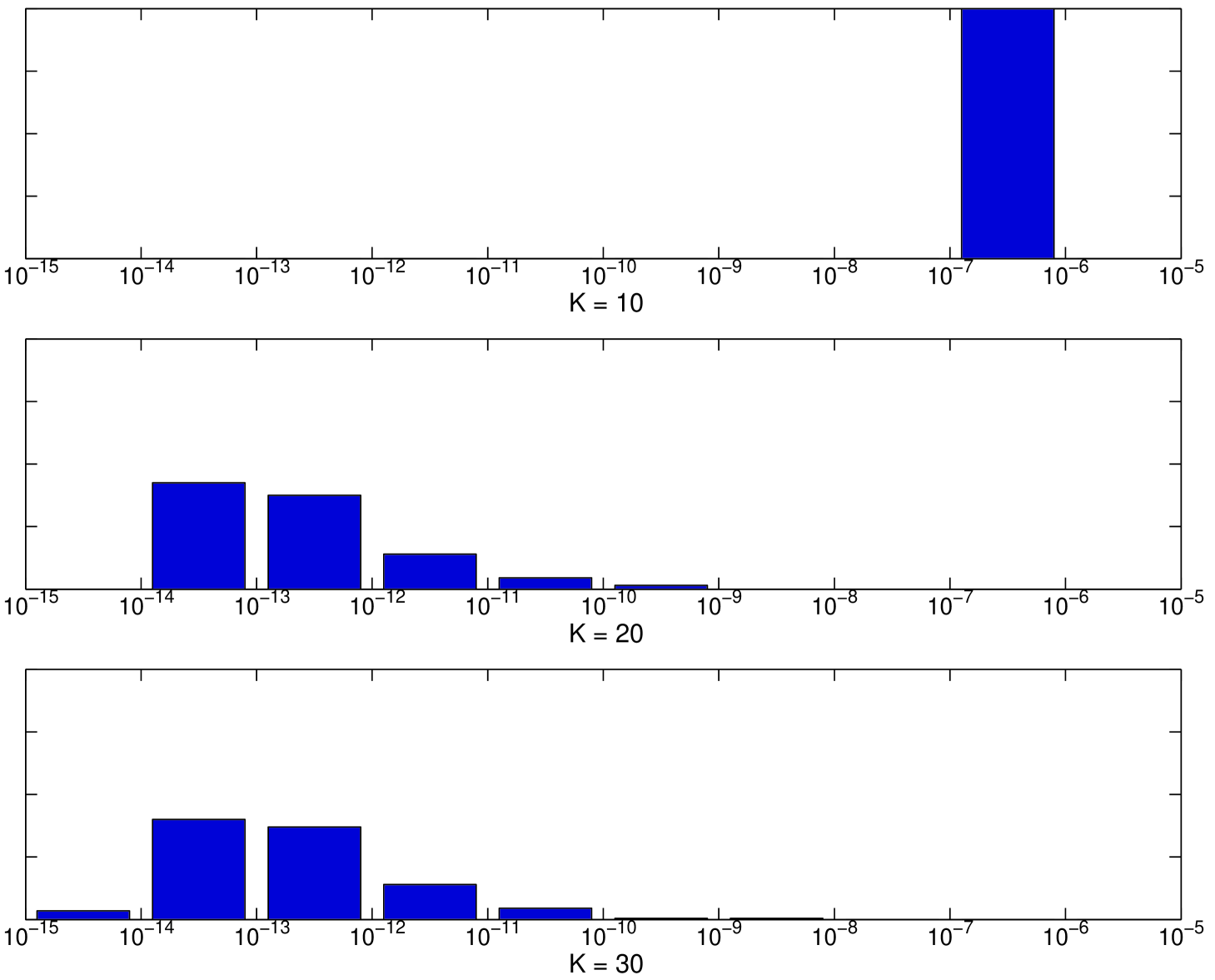

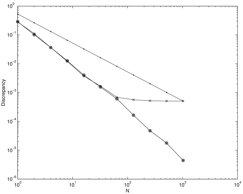
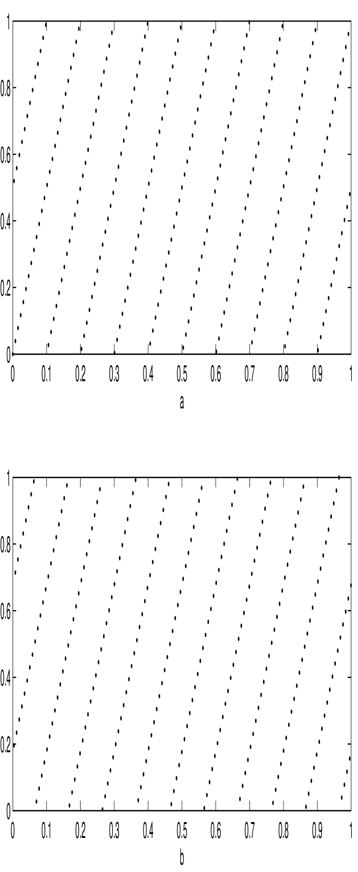
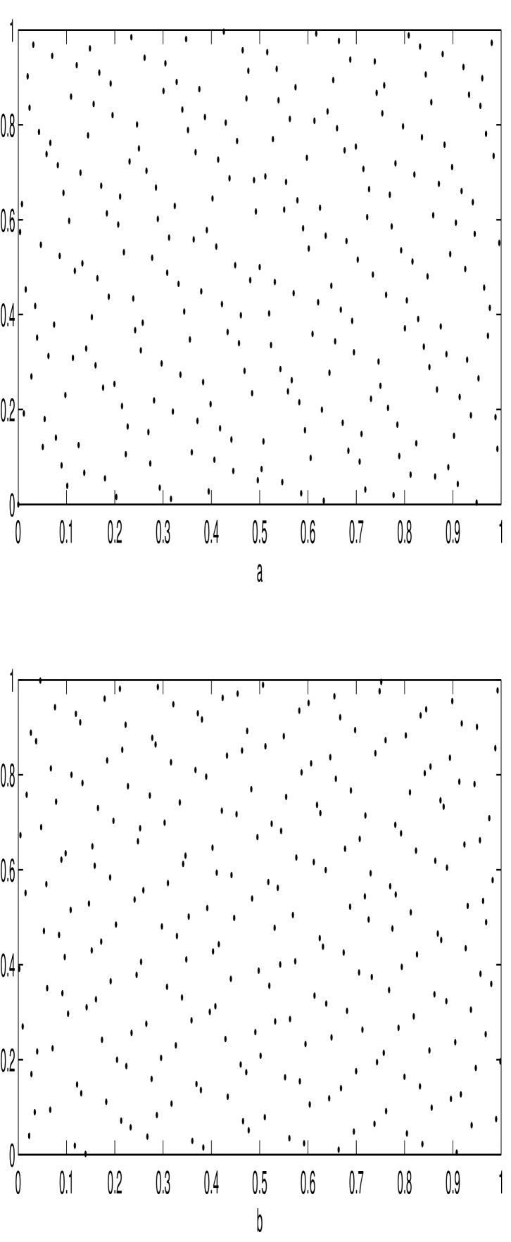
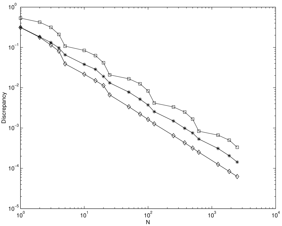
Figure 2.5 plots the discrepancies of the Faure sequence, the scrambled Faure sequence, and the tumbled Faure sequence. The number of scrambled digits, , is chosen to be 20, and 100 different replications have been performed. The choice of dimension is . Since the Faure sequence takes a base as a smallest prime number which is equal to or greater than , assigned to be . Therefore is chosen to be , where and . From Figure 2.5 scrambled sequences perform the best among all sequences and the tumbled sequence performs better than the original Faure sequence. Also notice that the scrambling and tumbling procedure help to flatten out the humps, which are present in the original sequence when the value of .
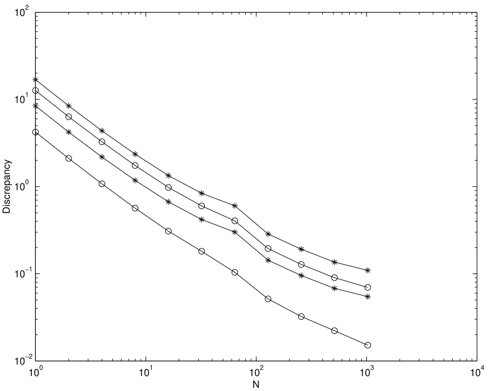
Figures 2.6–2.8 show the root mean square discrepancies of randomly scrambled -nets in base 2 with points that have been calculated by using 100 different replications. The choices of dimension are and . The number of scrambled digits, , is chosen to be 31.
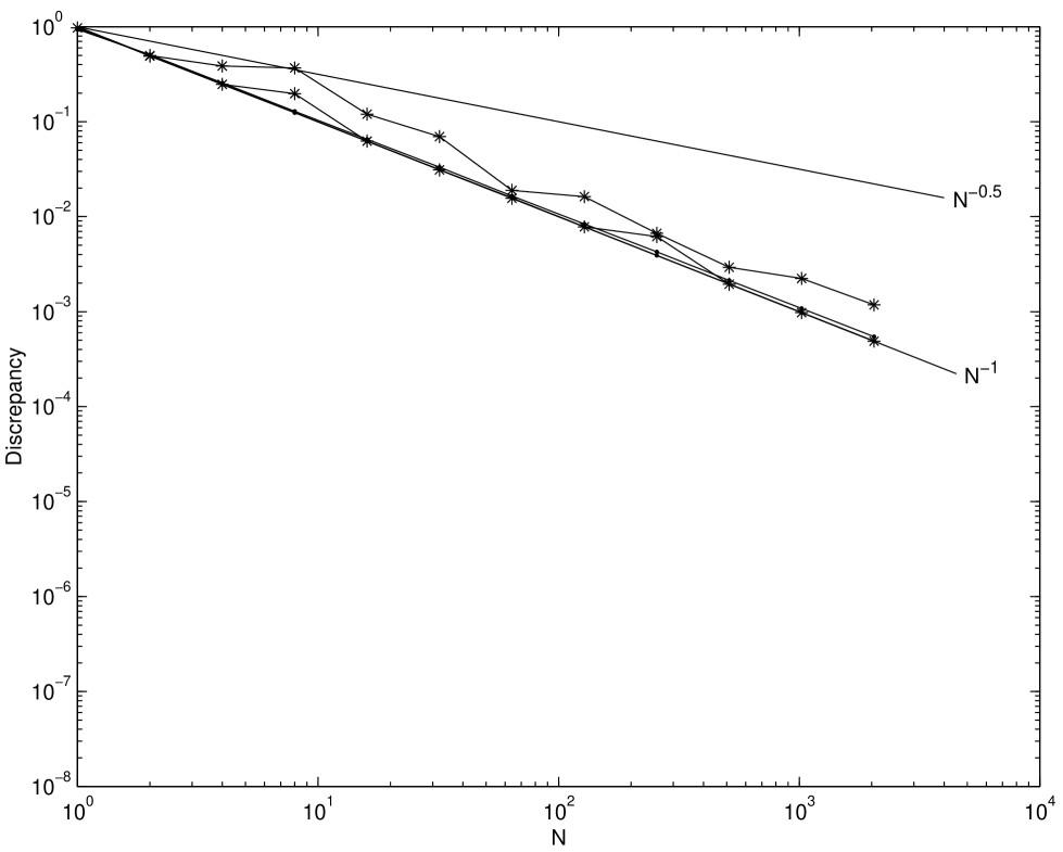
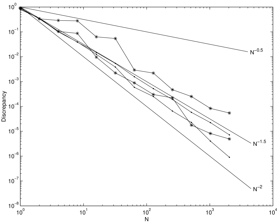
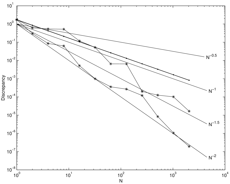
Theory predicts that the root mean square discrepancy of nets should decay as for , and as for . Figures 2.6–2.8 display this behavior, although for larger the asymptotic decay rate is only attained for large enough . However, even for smaller the discrepancy decays no worse than , the decay rate for a simple Monte Carlo sample.
The discrepancy of unscrambled nets does not attain the decay rate for . Although for these experiments all possible digits were scrambled, our experiment suggests that scrambling about digits is enough to obtain the benefits of scrambling. Scrambling more than this number does not improve the discrepancy but increases the time required to generate the scrambled points.
Chapter 3 The Distribution of the Discrepancy of Scrambled Digital -Nets
Recently, Loh [Loh01] proved that the scrambled net quadrature obeys a central limit theorem. This chapter studies the empirical distribution of the square discrepancy of scrambled nets and compares it to what one would expect from Loh’s central limit theorem. Here we use scrambling techniques mentioned in Chapter 2. Organization of the chapter is as follows. Section 3.1 provides a general description of the discrepancy with respect to the error of the quadrature and derives the theoretical asymptotic distribution of the square discrepancy of scrambled nets. Section 3.2 explains the procedure for fitting the empirical distribution of the square discrepancy of scrambled nets to the theoretical asymptotic distribution. Section 3.3 discusses the experimental results.
3.1 The Distribution of the Squared Discrepancy of Scrambled Nets
The discrepancy measures the uniformity of the distribution of a set of points and it can be interpreted as the maximum possible quadrature error over a unit ball of integrands. Since the discrepancy depends only on the quadrature rule, it is often used to compare different quadrature rules.
Let be the reproducing kernel for some Hilbert space of integrands whose domain is . To approximate the integral
one may use the quasi-Monte Carlo quadrature rule
where is some well-chosen set of points. The error of this rule is
and the square discrepancy is
where implies that the error functional is applied to the argument [Hic99].
The reproducing kernel may be written as the (usually infinite) sum
where is a basis for the Hilbert space of integrands [Wah90]. This implies that the discrepancy may be written as the sum [HW01]
By Loh’s central limit theorem it is known that each is asymptotically distributed as a normal random variable with mean zero. However, the are in general correlated.
By making an orthogonal transformation one may write
| (3.1) |
where the are independent random variables, and the are some constants. Note that if and then is approximately distributed as .
3.2 Fitting The Distribution Of The Square Discrepancy
Since equation (3.1) involves an infinite sum it must be further approximated in order to be computationally feasible. This is done by approximating all but the first terms by a constant:
| (3.2) |
where
Here denotes the expectation.
Let denote the random variable given by the square discrepancy of a scrambled net, and let denote the random variable given by the right hand side of (3.2). Let and denote the probability distribution functions of these two random variables, respectively. Ideally, one would find the and that minimize some loss function involving and , but these distributions are not known exactly. Thus, the optimal and are found by minimizing
| (3.3) |
Here,
and
the order statistic from a sample of scrambled net square discrepancies. Also,
the order statistic from a sample of independent and identically distributed drawings of , where
and is an odd multiple of . The logarithm is used in (3.3) because for a fixed and the square discrepancy values can vary by a factor of 100 or more, and it is not good for the larger values to unduly influence the fitted distribution.
Fitting the distribution of the square discrepancy by minimizing (3.3) relies on several approximations. The central limit theorem is invoked to obtain (3.1). The infinite sum is replaced by a finite one in (3.2). The probability distributions of each side of (3.2) are approximated by Monte Carlo sampling, and the two probability distributions are compared at only a finite number of points. In spite of these approximations the fitted distribution matches the observed distribution of the square discrepancy rather well.
3.3 Numerical Results
The discrepancy considered here is (1.1). With and the discrepancy can be rewritten as
| (3.4) |
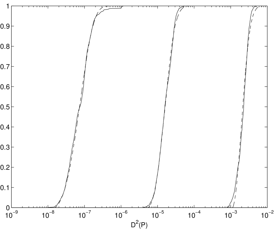
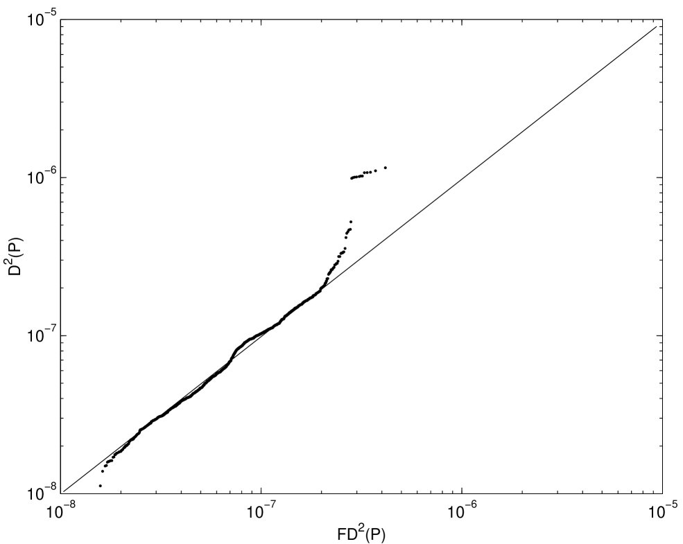
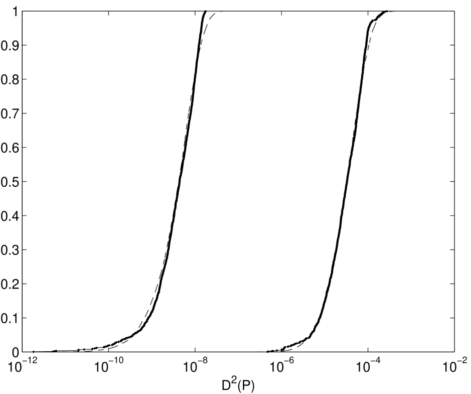
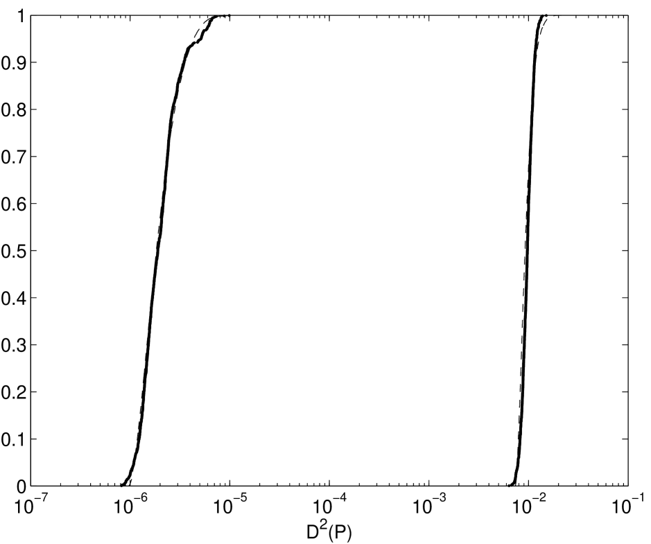
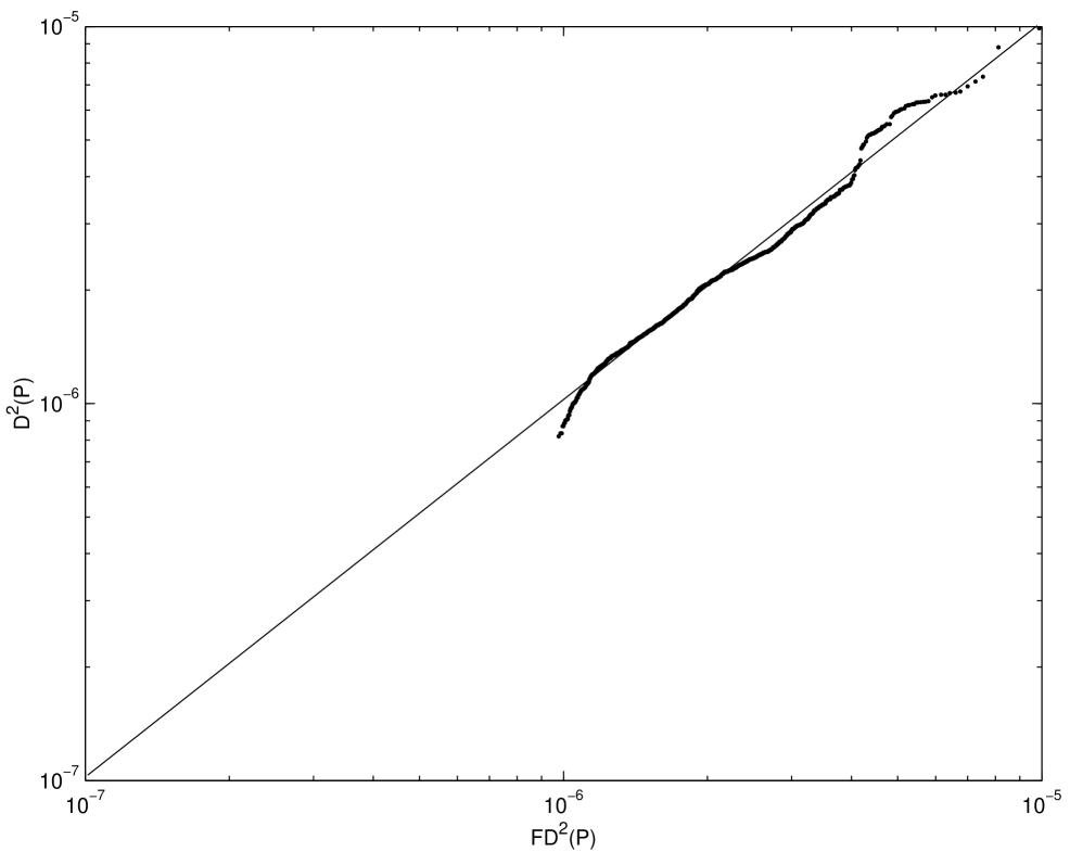
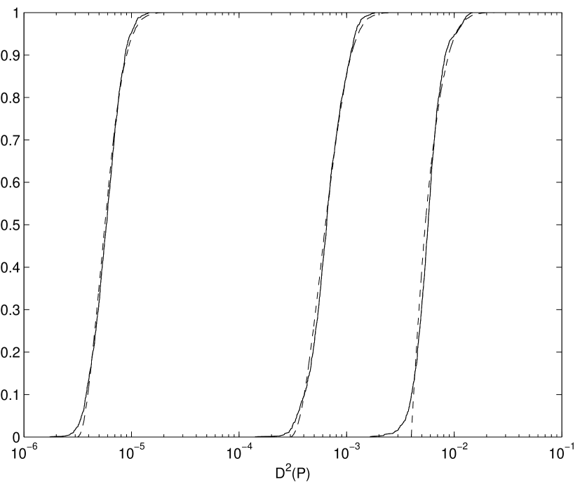
Figures 3.1 and 3.3 show the empirical distribution (dashed
line) of the square discrepancy of scrambled nets and its fitted value
(thin line). The fit is based on replications of the
scrambled Sobol’ [BF88, HH01], Niederreiter-Xing,
and Faure nets, , and or . The optimization was done by
using MATLAB’s fminsearch
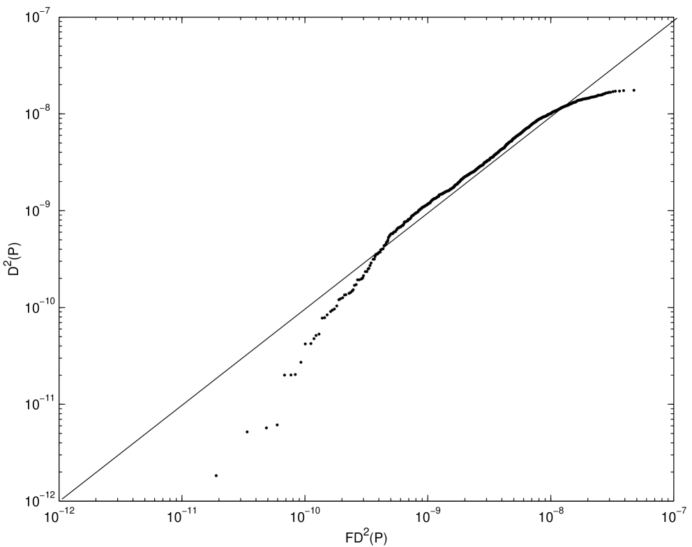
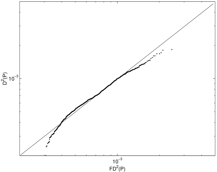
function. The fits are good in the middle of the distributions, but
off in the tails. Moreover the Q-Q plots of the empirical and fitted
distributions bear this out.
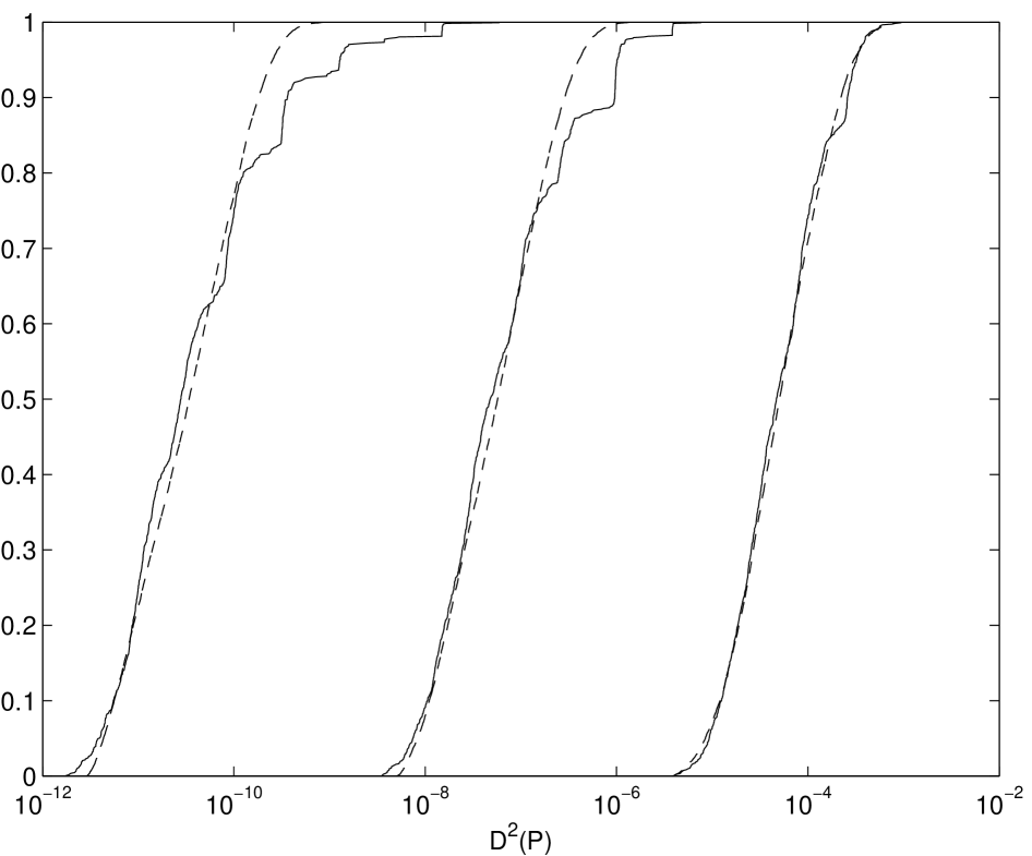
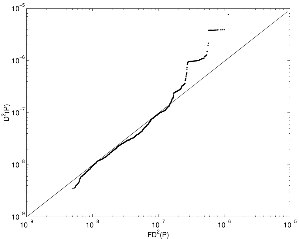
There are several humps in the empirical distribution of the square discrepancy for . Moreover as increases, the number of humps increases. However, these humps are less noticeable as the dimension increases.
The humps can be explained as follows: The scrambling technique used here, as described in Chapter 2, scrambles the generator matrices of these digital nets and also gives them a digital shift. Since this technique preserves the digital nature of the nets, it can be shown that for the sum of the digits of points numbered , is zero modulo . However, for Owen’s original scrambling this is not necessarily the case. For example, in one dimension Owen’s scrambling is equivalent to Latin hypercube sampling. Figures 3.9 and 3.10 show the empirical distribution of the square discrepancy for a scrambled one-dimensional Sobol’ net and for Latin hypercube sampling. Since the base of the Sobol’ sequence is the difference in the two graphs emerges for . Note that although the distributions of the square discrepancy for Owen’s original scrambling and the variant used here are somewhat different, the means of the two distributions are the same.
The square discrepancy can be written as a sum of polynomials in :
Then the sum of polynomials can be rearranged as
where measures the uniformity of all -dimensional projections of [Hic98]. A computationally efficient method for obtaining all of the is to compute for different values of and then perform polynomial interpolation. Specifically Newton’s divided difference formula has been applied for polynomial interpolation.
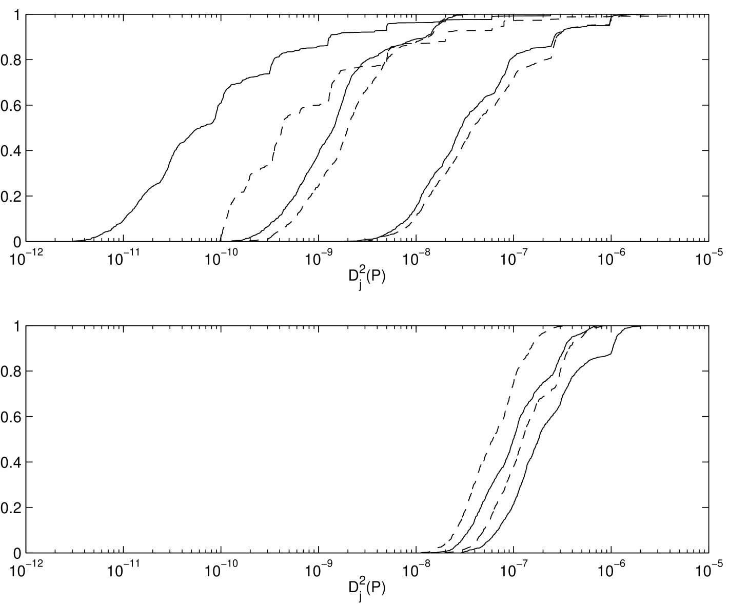
Figure 3.11 plots the distribution of for -dimensional scrambled Sobol’ and scrambled Niederreiter-Xing nets [NX96, NX98] for . The -values for these nets are 3 and 2 respectively. From this figure the scrambled Sobol’ net has smaller for and the scrambled Niederreiter-Xing sequence has smaller for . This means that for integrands that can be well approximated by sums of one and two-dimensional functions, the Sobol’ net will tend to give small quadrature error even though it has larger value.
Here the empirical distribution of randomly shifted lattice points has been investigated as well (see Figures 3.12 and 3.13). Here we use a Korobov type rank-1 lattice with generator [HHLL01]. Although there is no known theory on the distribution of the randomly shifted lattice points, the fitted distribution of the form used for nets seems to work well for large enough .
Chapter 4 -parameter Optimization for Digital -nets by Evolutionary Computation
So far most -nets are generated by number theoretic methods. However, in this chapter we use optimization methods to generate a digital -net. This chapter explains a procedure for finding good generator matrices of digital -nets. Here we consider imbedded generator matrices, that is one set of generator matrices is used for any and . Many well known generator matrices of digital -nets are imbedded matrices, namely Sobol’ and Niederreiter. Such imbedded matrices have a certain advantage that the user needs only one set of matrices rather than several different sets of matrices that work for different or . Finding good imbedded nets is more difficult than finding nets with fixed and .
In Chapter 1 we introduced the definition of as the quality measure of -nets and -sequences in terms of an elementary interval in base . In this chapter the quality parameters are expressed as the number of linearly independent rows of generator matrices for digital -nets, which can be computed from the generator matrices. Section 4.2 introduces the basic concept of evolutionary computation that is used for solving optimization problems for finding better nets. Section 4.3 explains the detail methodology. Finally we report on some numerical results of new generator matrices by making comparisons to other well known generator matrices of digital -nets.
4.1 Digital -Nets and -Sequences
For a prime number the quality of a digital sequence is expressed by its -value, which can be determined from the generator matrices. For any positive integer let be the row vector containing the first columns of the row of . Let be an integer, , such that for all -vectors of non-negative integers with ,
| (4.1) |
where is a finite field in mod . Then for any non-negative integer and any with , the set defined by (1.10) is a -net in base . (Note that a -net is the same as a -net.) If the same value of holds for all non-negative integers , then the digital sequence is a -sequence.
An efficient algorithm is available for the determination of the quality parameter of a digital net in the binary case. More detailed explanations can be found in [Sch99a].
4.2 Evolutionary Computation
Evolutionary Computation [Hei00] is an algorithm which is based on the principles of a natural evolution as a method to solve parameter optimization problems. An evolutionary algorithm (EA) constructs a population of candidate solutions for the problem at hand. The solutions are evolving by iteratively applying a set of stochastic operators, (or genetic operators) known as recombination, mutation, reproduction and selection. During the iterating process (or evolving process) each individual in the population receives a measure of its fitness in the environment.
In EA each individual represents a potential solution to the problem at hand, and in any evolution program, is implemented as some (possibly complex structure) data structure. Each solution is evaluated to give some measures of its “fitness”, then the new population is formed by selecting the more fit individuals. Some members of the new population undergo transformations by means of “genetic” operators to form a new solution. There is a unary transformation (mutation type), which creates new individuals by a small change in a single individual. Higher order transformation (crossover type) creates new individuals by combining parts from several individuals. After some number of generations the program converges to a solution which might be a near-optimum solution. Traditionally the data structure of EA is binary representations and an operator set consisting only of binary crossover and binary mutation which is not suitable for many applications.
However a richer set of data structure (for chromosome representation) together with an expanded set of a genetic operators has been introduced. The chromosomes need not be represented by bit-strings. Instead it could be floating number representation. The alternation process including other “genetic” operators appropriates for the given structure and the given problem. These variations include variables length string, richer than binary string. These modified genetic operators meet the needs of particular applications.
The following is a detailed description of stochastic operators in EA.
-
•
Recombination perturbs the solution by decomposing distinct solutions and then randomly mixes their parts to form a novel solution.
-
•
Mutation might play important role that introduces further diversity while the algorithm is running by randomly (or stochastically) perturbing a candidate solution, since a large amount of diversity is usually introduced only at the start of the algorithm by randomizing the genes in the population.
-
•
Selection evaluates the fitness value of the individuals and purges poor solutions from population. It resembles the fitness of survivors in nature.
-
•
Reproduction focuses attention on high fitness individuals and replicates the most successful solutions found in a population.
The resulting process tends to find globally optimal solutions to the problem much in the same way as the natural populations of organisms adapt to their surrounding environment.
A variety of evolutionary algorithms has been proposed. The major ones are genetic algorithms [Gol89], evolutionary programming [Fog95], evolutionary strategies [Kur92], and genetic programming. They all share the common conceptual base of simulating the evolution of individual structures via processes of stochastic operators which are mentioned earlier. They have been applied to various problems where there was no other known problem solving strategy, and the problem domain is NP-complete. That is the usual place where EAs solve the problem by heuristically finding solutions where others fail.
PSEUDO CODE
Algorithm EA is
*********************************************************************
// start with an initial time
Time := 0;
// initialize a usually random population of individuals
initpopulation Pop;
// evaluate fitness of all initial individuals in population
evaluate Pop;
// test for termination criterion (time, fitness, etc)
While not done do
// select sub-population for offspring production
SPop := selectparents Pop;
// recombine the ”genes” of selected parents
recombine SPop;
// perturb the mated population randomly or stochastically
mutate SPop;
// evaluate its new fitness
evaluate SPop;
// select the survivors from the actual fitness
Pop := survive Pop,SPop;
// increase the time counter
Time := Time+1;
*********************************************************************
4.3 Searching Method
Searching for finding good generator matrices can be considered as solving a combinatorial optimization problem. As the size of and increases, the possible solutions of the problem become exponentially large, . Evolutionary computation is one of the methods for solving such problem. In this section we describe the searching procedure for finding good digital -nets by an evolutionary computation strategy.
4.3.1 Environment Setting
Considering generator matrix where .
First, we define an individual as . Each sub population can be expressed as where is the size of cells. Here we consider the matrix as a upper triangular matrix with all diagonal entries are one. Notice that we only consider the case . Then the size of becomes . The following explains the correspondence between and .
4.3.2 Searching Strategy
In previous section, we define an individual . However looking at optimization problem as a whole, the population becomes where and is the number of individuals. In this problem we choose . The followings explain the detail setting of stochastic operators.
(a) Recombination : Two points crossover has been adopted. The recombination only occurs for the same among s. The selection of the locations of crossover is chosen randomly within first half for the first location and second half for two second location.
(b) Mutation : 5 % of randomly selected positions are assigned to perform mutation.
(c) Selection : Best 30 % of individuals are selected based on a given objective function.
(d) Reproduction : The best individuals are selected from the current generation to remain as the part of the next generation. And the rest of the next generation is produced based on the replication of the best individuals of the current generation. Since we are keeping the best previous individuals as themselves, aging has been introduced that each individual will be removed when the individuals are survived more than certain length of period.
4.3.3 Objective Function
There are various objective functions that can be used in this problem.
Here we select an objective function as the sum of values for
dimensional projections. The details are following.
Let be the smallest
for which generates a -net
that the values of the digital -net generated by
where is the top sub-matrix.
For given , we can use these matrices to generate -nets and extend the nets for and .
Finally the objective function is written as
Our goal is finding the generator matrices that obtain the smaller values.
4.4 Numerical Results
The newly obtained digital -net by an evolutionary computation is named as the EC net. The exact quality parameters of the generator matrices were calculated by using the program provided by Schmid [Sch99a]. Notice that initial populations are selected partially at random and partially by taking Sobol’ generator matrices and randomly choosing the matrices. Table 4.1 shows the values of generator matrices of EC sequence. Here the is defined as following:
The same definition is applied for the remaining section.
| s | m | 1 | 2 | 3 | 4 | 5 | 6 | 7 | 8 | 9 | 10 | 11 | 12 | 13 | 14 | 15 | 16 | 17 | 18 | 19 | 20 |
|---|---|---|---|---|---|---|---|---|---|---|---|---|---|---|---|---|---|---|---|---|---|
| 1 | 0 | 0 | 0 | 0 | 0 | 0 | 0 | 0 | 0 | 0 | 0 | 0 | 0 | 0 | 0 | 0 | 0 | 0 | 0 | 0 | |
| 2 | 0 | 0 | 0 | 0 | 0 | 0 | 0 | 0 | 0 | 0 | 0 | 0 | 0 | 0 | 0 | 0 | 0 | 0 | 0 | 0 | |
| 3 | 0 | 1 | 1 | 1 | 1 | 1 | 1 | 1 | 1 | 1 | 1 | 1 | 1 | 1 | 1 | 1 | 1 | 1 | 1 | 1 | |
| 4 | 0 | 1 | 2 | 2 | 2 | 3 | 3 | 3 | 3 | 3 | 3 | 3 | 3 | 3 | 3 | 3 | 3 | 3 | 3 | 3 | |
| 5 | 0 | 1 | 2 | 2 | 2 | 3 | 3 | 3 | 3 | 3 | 4 | 4 | 5 | 5 | 5 | 5 | 5 | 5 | 5 | 5 | |
| 6 | 0 | 1 | 2 | 2 | 3 | 3 | 4 | 5 | 5 | 5 | 6 | 6 | 6 | 6 | 7 | 7 | 7 | 7 | 7 | 7 | |
| 7 | 0 | 1 | 2 | 3 | 3 | 3 | 4 | 5 | 5 | 5 | 6 | 6 | 6 | 6 | 7 | 7 | 7 | 7 | 8 | 8 | |
| 8 | 0 | 1 | 2 | 3 | 3 | 3 | 4 | 5 | 5 | 6 | 7 | 7 | 7 | 8 | 9 | 9 | 9 | 9 | 9 | 9 | |
| 9 | 0 | 1 | 2 | 3 | 3 | 4 | 4 | 5 | 6 | 6 | 7 | 7 | 7 | 8 | 9 | 9 | 9 | 10 | 11 | 11 | |
| 10 | 0 | 1 | 2 | 3 | 3 | 4 | 4 | 5 | 6 | 7 | 7 | 8 | 9 | 9 | 9 | 9 | 9 | 10 | 11 | 11 | |
| 11 | 0 | 1 | 2 | 3 | 4 | 5 | 5 | 5 | 6 | 7 | 7 | 8 | 9 | 10 | 10 | 10 | 10 | 11 | 11 | 11 | |
| 12 | 0 | 1 | 2 | 3 | 4 | 5 | 5 | 5 | 6 | 7 | 8 | 8 | 9 | 10 | 10 | 10 | 10 | 11 | 12 | 13 | |
| 13 | 0 | 1 | 2 | 3 | 4 | 5 | 5 | 6 | 6 | 7 | 8 | 8 | 9 | 10 | 10 | 10 | 10 | 11 | 12 | 13 | |
| 14 | 0 | 1 | 2 | 3 | 4 | 5 | 5 | 6 | 7 | 7 | 8 | 8 | 9 | 10 | 11 | 12 | 13 | 13 | 13 | 13 | |
| 15 | 0 | 1 | 2 | 3 | 4 | 5 | 5 | 6 | 7 | 7 | 8 | 8 | 9 | 10 | 11 | 12 | 13 | 13 | 13 | 13 | |
| 16 | 0 | 1 | 2 | 3 | 4 | 5 | 5 | 6 | 7 | 7 | 8 | 9 | 10 | 10 | 11 | 12 | 13 | 13 | 13 | 13 | |
| 17 | 0 | 1 | 2 | 3 | 4 | 5 | 5 | 6 | 7 | 7 | 8 | 9 | 10 | 10 | 11 | 12 | 13 | 13 | 13 | 13 | |
| 18 | 0 | 1 | 2 | 3 | 4 | 5 | 5 | 6 | 7 | 7 | 8 | 9 | 10 | 10 | 11 | 12 | 13 | 13 | 14 | 15 | |
| 19 | 0 | 1 | 2 | 3 | 4 | 5 | 5 | 6 | 7 | 7 | 8 | 9 | 10 | 10 | 11 | 12 | 13 | 13 | 14 | 15 | |
| 20 | 0 | 1 | 2 | 3 | 4 | 5 | 5 | 6 | 7 | 7 | 8 | 9 | 10 | 10 | 11 | 12 | 13 | 13 | 14 | 15 | |
| 21 | 0 | 1 | 2 | 3 | 4 | 5 | 6 | 6 | 7 | 7 | 8 | 9 | 10 | 10 | 11 | 12 | 13 | 13 | 14 | 15 | |
| 22 | 0 | 1 | 2 | 3 | 4 | 5 | 6 | 6 | 7 | 7 | 8 | 9 | 10 | 10 | 11 | 12 | 13 | 13 | 14 | 15 | |
| 23 | 0 | 1 | 2 | 3 | 4 | 5 | 6 | 6 | 7 | 7 | 8 | 9 | 10 | 11 | 12 | 12 | 13 | 13 | 14 | 15 | |
| 24 | 0 | 1 | 2 | 3 | 4 | 5 | 6 | 6 | 7 | 7 | 8 | 9 | 10 | 11 | 12 | 12 | 13 | 13 | 14 | 15 | |
| 25 | 0 | 1 | 2 | 3 | 4 | 5 | 6 | 6 | 7 | 7 | 8 | 9 | 10 | 11 | 12 | 12 | 13 | 13 | 14 | 15 | |
| 26 | 0 | 1 | 2 | 3 | 4 | 5 | 6 | 6 | 7 | 7 | 8 | 9 | 10 | 11 | 12 | 12 | 13 | 13 | 14 | 15 | |
| 27 | 0 | 1 | 2 | 3 | 4 | 5 | 6 | 6 | 7 | 7 | 8 | 9 | 10 | 11 | 12 | 12 | 13 | 13 | 14 | 15 | |
| 28 | 0 | 1 | 2 | 3 | 4 | 5 | 6 | 6 | 7 | 7 | 8 | 9 | 10 | 11 | 12 | 12 | 13 | 13 | 14 | 15 | |
| 29 | 0 | 1 | 2 | 3 | 4 | 5 | 6 | 6 | 7 | 7 | 8 | 9 | 10 | 11 | 12 | 12 | 13 | 13 | 14 | 15 | |
| 30 | 0 | 1 | 2 | 3 | 4 | 5 | 6 | 6 | 7 | 7 | 8 | 9 | 10 | 11 | 12 | 12 | 13 | 13 | 14 | 15 | |
| 31 | 0 | 1 | 2 | 3 | 4 | 5 | 6 | 6 | 7 | 7 | 8 | 9 | 10 | 11 | 12 | 12 | 13 | 13 | 14 | 15 | |
| 32 | 0 | 1 | 2 | 3 | 4 | 5 | 6 | 6 | 7 | 7 | 8 | 9 | 10 | 11 | 12 | 12 | 13 | 13 | 14 | 15 | |
| 33 | 0 | 1 | 2 | 3 | 4 | 5 | 6 | 6 | 7 | 7 | 8 | 9 | 10 | 11 | 12 | 12 | 13 | 13 | 14 | 15 | |
| 34 | 0 | 1 | 2 | 3 | 4 | 5 | 6 | 6 | 7 | 7 | 8 | 9 | 10 | 11 | 12 | 13 | 14 | 15 | 15 | 15 | |
| 35 | 0 | 1 | 2 | 3 | 4 | 5 | 6 | 6 | 7 | 7 | 8 | 9 | 10 | 11 | 12 | 13 | 14 | 15 | 15 | 15 | |
| 36 | 0 | 1 | 2 | 3 | 4 | 5 | 6 | 6 | 7 | 7 | 8 | 9 | 10 | 11 | 12 | 13 | 14 | 15 | 15 | 15 | |
| 37 | 0 | 1 | 2 | 3 | 4 | 5 | 6 | 6 | 7 | 7 | 8 | 9 | 10 | 11 | 12 | 13 | 14 | 15 | 15 | 15 | |
| 38 | 0 | 1 | 2 | 3 | 4 | 5 | 6 | 6 | 7 | 7 | 8 | 9 | 10 | 11 | 12 | 13 | 14 | 15 | 15 | 15 | |
| 39 | 0 | 1 | 2 | 3 | 4 | 5 | 6 | 6 | 7 | 8 | 9 | 10 | 10 | 11 | 12 | 13 | 14 | 15 | 15 | 15 | |
| 40 | 0 | 1 | 2 | 3 | 4 | 5 | 6 | 7 | 7 | 8 | 9 | 10 | 10 | 11 | 12 | 13 | 14 | 15 | 15 | 15 |
Table 4.2 shows the comparison of values between generator matrices of Sobol’ and EC nets for and . The value for Sobol’ sequence is and EC sequence is . For the comparison of overall values, if the two methods have the same values then the entry is marked as *. But if one net is better, which means having a smaller value, then it is marked as the initial of the better net. Also if the difference of value is greater than then the difference is indicated in front of the initial. For example, means the generator matrices of EC sequence has a smaller value than Sobol’ sequence by . From the table 4.2, there are some entries that Sobol’ is better than EC and vice versa. However EC sequence has smaller values than the Sobol’ sequence. The EC sequence tends to have smaller values that the Sobol’ sequence for larger and .
| s | m | 1 | 2 | 3 | 4 | 5 | 6 | 7 | 8 | 9 | 10 | 11 | 12 | 13 | 14 | 15 | 16 | 17 | 18 | 19 | 20 |
|---|---|---|---|---|---|---|---|---|---|---|---|---|---|---|---|---|---|---|---|---|---|
| 10 | * | * | * | * | * | * | * | * | * | * | S | * | S | S | S | * | * | * | * | * | |
| 11 | * | * | * | * | * | S | S | * | * | S | * | * | * | * | E | 2E | 2E | E | E | E | |
| 12 | * | * | * | * | * | S | * | * | * | * | * | * | * | * | E | 2E | 2E | E | * | S | |
| 13 | * | * | * | * | * | S | * | S | * | * | * | * | * | * | E | 2E | 2E | E | * | * | |
| 14 | * | * | * | * | * | S | * | S | S | * | * | * | * | * | * | * | S | * | E | E | |
| 15 | * | * | * | * | * | S | * | S | S | * | * | E | E | * | * | * | S | * | E | E | |
| 16 | * | * | * | * | * | S | * | S | S | * | * | * | * | * | * | * | S | * | E | E | |
| 17 | * | * | * | * | * | S | * | S | S | * | * | * | * | * | * | * | S | * | E | E | |
| 18 | * | * | * | * | * | S | * | * | * | E | * | * | * | E | E | E | E | E | * | S | |
| 19 | * | * | * | * | * | S | * | * | * | E | * | * | * | E | E | E | E | E | * | S | |
| 20 | * | * | * | * | * | S | * | * | * | E | * | * | * | E | E | E | E | E | * | S | |
| 21 | * | * | * | * | * | S | S | * | * | E | * | * | * | E | E | E | E | E | * | S | |
| 22 | * | * | * | * | * | S | S | * | * | E | * | * | * | E | E | E | E | E | * | S | |
| 23 | * | * | * | * | * | S | S | * | * | E | * | * | * | * | * | E | E | E | * | S | |
| 24 | * | * | * | * | * | S | S | * | * | E | * | * | * | * | * | E | E | E | * | S | |
| 25 | * | * | * | * | * | S | S | * | * | E | * | * | * | * | * | E | E | E | * | S | |
| 26 | * | * | * | * | * | S | S | * | * | E | * | * | * | * | * | E | E | E | * | S | |
| 27 | * | * | * | * | * | S | S | * | * | E | * | * | * | * | * | E | E | E | * | S | |
| 28 | * | * | * | * | * | S | S | * | * | E | * | * | * | * | * | E | E | E | * | S | |
| 29 | * | * | * | * | * | S | S | * | * | E | * | * | * | * | * | E | E | E | * | S | |
| 30 | * | * | * | * | * | S | S | * | * | E | * | * | * | * | * | E | E | E | * | S | |
| 31 | * | * | * | * | * | S | S | * | * | E | E | E | E | * | * | E | E | E | * | * | |
| 32 | * | * | * | * | * | S | S | * | * | E | E | E | E | * | * | E | E | E | * | * | |
| 33 | * | * | * | * | * | * | S | * | * | E | E | E | E | * | * | E | E | E | * | * | |
| 34 | * | * | * | * | * | * | * | * | * | E | E | E | E | * | * | * | * | S | S | * | |
| 35 | * | * | * | * | * | * | * | E | * | E | E | E | E | * | * | * | * | S | * | * | |
| 36 | * | * | * | * | * | * | * | E | E | 2E | E | E | E | * | * | * | * | S | * | * | |
| 37 | * | * | * | * | * | * | * | E | E | 2E | E | E | E | * | * | * | * | * | E | 2E | |
| 38 | * | * | * | * | * | * | * | E | E | 2E | E | E | E | * | * | * | * | * | E | 2E | |
| 39 | * | * | * | * | * | * | * | E | E | E | * | * | E | * | * | * | * | * | E | 2E | |
| 40 | * | * | * | * | * | * | * | * | E | E | * | * | E | * | * | * | * | * | E | 2E |
We also compare the generator matrices of Niederreiter-Xing sequence with EC sequence. However, notice that the generator matrices of Niederreiter-Xing sequence are originally not constructed as imbedded matrices like EC and Sobol’ sequences do. Therefore there are different generator matrices available for different . Here we compute the values of the generator matrices of Niederreiter-Xing like other imbedded matrices. Two matrices are chosen for comparison, “nxs18m30” for and “nxs32m40” for . The generator matrices are obtained from [Pir02].
From tables 4.3 and 4.4, the EC sequence obtains smaller values than Niederreiter-Xing sequence, and the differences are larger for smaller . It is understandable that the generator matrices are constructed best for fixed dimension like and in this example. However the tables show EC sequence even obtains smaller values for .
| s | m | 1 | 2 | 3 | 4 | 5 | 6 | 7 | 8 | 9 | 10 | 11 | 12 | 13 | 14 | 15 | 16 | 17 | 18 | 19 | 20 |
|---|---|---|---|---|---|---|---|---|---|---|---|---|---|---|---|---|---|---|---|---|---|
| 1 | E | 2E | 3E | 4E | 5E | 6E | 6E | 6E | 6E | 6E | 6E | 6E | 6E | 6E | 6E | 6E | 6E | 6E | 6E | 6E | |
| 2 | E | 2E | 3E | 4E | 5E | 6E | 6E | 6E | 6E | 6E | 7E | 8E | 8E | 8E | 8E | 8E | 8E | 8E | 8E | 8E | |
| 3 | E | E | 2E | 3E | 4E | 5E | 5E | 5E | 5E | 5E | 6E | 7E | 7E | 7E | 7E | 7E | 7E | 7E | 7E | 7E | |
| 4 | E | E | E | 2E | 3E | 3E | 3E | 3E | 3E | 3E | 4E | 5E | 5E | 6E | 6E | 6E | 6E | 6E | 6E | 6E | |
| 5 | E | E | E | 2E | 3E | 3E | 3E | 3E | 3E | 3E | 3E | 4E | 3E | 4E | 4E | 4E | 4E | 5E | 5E | 5E | |
| 6 | E | E | E | 2E | 2E | 3E | 2E | E | E | E | E | 2E | 2E | 3E | 3E | 4E | 4E | 4E | 4E | 4E | |
| 7 | E | E | E | E | 2E | 3E | 2E | E | E | E | E | 2E | 2E | 3E | 3E | 4E | 4E | 4E | 4E | 4E | |
| 8 | E | E | E | E | 2E | 3E | 2E | E | E | E | E | E | E | E | E | 2E | 2E | 3E | 3E | 3E | |
| 9 | E | E | E | E | 2E | 2E | 2E | E | * | E | E | E | 2E | E | E | 2E | 2E | 2E | E | E | |
| 10 | E | E | E | E | 2E | 2E | 2E | E | * | * | E | * | * | * | E | 2E | 3E | 3E | 3E | 4E | |
| 11 | E | E | E | E | E | E | E | E | * | * | E | * | * | N | * | E | 2E | 2E | 3E | 4E | |
| 12 | E | E | E | E | E | E | E | E | E | E | E | 2E | 2E | 2E | 3E | 4E | 4E | 3E | 2E | 2E | |
| 13 | E | E | E | E | E | E | E | * | E | E | E | 2E | 2E | 2E | 3E | 4E | 4E | 3E | 2E | 2E | |
| 14 | E | E | E | E | E | E | E | E | * | E | E | 2E | 2E | 2E | 2E | 2E | E | E | E | 2E | |
| 15 | E | E | E | E | E | E | E | E | * | E | E | 2E | 2E | 2E | 2E | 2E | E | E | E | 2E | |
| 16 | E | E | E | E | E | E | E | E | * | E | E | E | E | 2E | 2E | 2E | E | E | E | 2E | |
| 17 | E | E | E | E | E | E | E | E | * | E | E | E | E | 2E | 2E | 2E | E | E | E | 2E | |
| 18 | E | E | E | E | E | E | E | E | * | E | E | E | E | 2E | 2E | 2E | E | E | * | * |
| s | m | 1 | 2 | 3 | 4 | 5 | 6 | 7 | 8 | 9 | 10 | 11 | 12 | 13 | 14 | 15 | 16 | 17 | 18 | 19 | 20 |
|---|---|---|---|---|---|---|---|---|---|---|---|---|---|---|---|---|---|---|---|---|---|
| 1 | E | 2E | 3E | 4E | 4E | 4E | 4E | 4E | 4E | 4E | 4E | 4E | 4E | 4E | 4E | 4E | 4E | 4E | 4E | 4E | |
| 2 | E | 2E | 3E | 4E | 4E | 4E | 4E | 4E | 4E | 4E | 4E | 4E | 4E | 4E | 4E | 4E | 4E | 4E | 4E | 4E | |
| 3 | E | E | 2E | 3E | 3E | 3E | 3E | 3E | 4E | 4E | 4E | 4E | 4E | 5E | 5E | 5E | 5E | 5E | 5E | 5E | |
| 4 | E | E | E | 2E | 2E | 2E | 3E | 3E | 3E | 3E | 4E | 5E | 6E | 6E | 6E | 6E | 6E | 6E | 6E | 6E | |
| 5 | E | E | E | 2E | 2E | 2E | 3E | 3E | 3E | 3E | 3E | 4E | 4E | 4E | 4E | 4E | 4E | 4E | 4E | 4E | |
| 6 | E | E | E | 2E | E | 2E | 2E | 2E | 3E | 3E | 2E | 2E | 3E | 3E | 2E | 2E | 3E | 4E | 5E | 6E | |
| 7 | E | E | E | E | E | 2E | 2E | 2E | 3E | 3E | 2E | 3E | 3E | 3E | 2E | 2E | 3E | 4E | 4E | 5E | |
| 8 | E | E | E | E | E | 2E | 2E | 2E | 3E | 2E | E | 2E | 2E | E | * | * | E | 2E | 3E | 4E | |
| 9 | E | E | E | E | E | E | 2E | 2E | 2E | 2E | E | 2E | 2E | E | * | * | E | E | E | 2E | |
| 10 | E | E | E | E | E | E | 2E | 2E | 2E | E | E | E | * | * | * | E | E | E | E | 2E | |
| 11 | E | E | E | E | * | * | E | 2E | 2E | E | E | E | * | N | * | * | * | * | E | 2E | |
| 12 | E | E | E | E | * | * | E | 2E | 2E | E | * | E | * | N | * | * | * | * | * | * | |
| 13 | E | E | E | E | * | * | E | E | 2E | E | * | E | * | N | * | * | E | E | * | * | |
| 14 | E | E | E | E | * | * | E | E | E | E | * | E | * | * | N | 2E | 2E | N | N | * | |
| 15 | E | E | E | E | * | * | E | E | E | E | * | E | E | E | * | N | N | N | * | E | |
| 16 | E | E | E | E | * | * | E | E | E | E | * | * | * | E | * | N | N | N | * | E | |
| 17 | E | E | E | E | * | * | E | E | E | E | * | * | * | E | * | N | N | * | E | E | |
| 18 | E | E | E | E | * | * | E | E | E | E | * | * | * | E | * | N | N | * | * | N | |
| 19 | E | E | E | E | * | * | E | E | E | E | * | * | * | E | * | N | N | * | * | N | |
| 20 | E | E | E | E | * | * | E | E | E | E | * | * | * | E | * | N | N | * | * | N | |
| 21 | E | E | E | E | * | * | * | E | E | E | * | * | * | E | * | N | N | * | * | N | |
| 22 | E | E | E | E | * | * | * | E | E | 2E | E | * | * | E | * | N | N | * | * | N | |
| 23 | E | E | E | E | * | * | * | E | E | 2E | E | * | * | * | N | * | N | * | * | * | |
| 24 | E | E | E | E | * | * | * | E | E | 2E | E | * | * | * | N | * | N | * | * | * | |
| 25 | E | E | E | E | * | * | * | E | E | 2E | E | * | * | * | * | E | * | * | * | * | |
| 26 | E | E | E | E | * | * | * | E | E | 2E | E | * | * | * | * | E | * | * | * | * | |
| 27 | E | E | E | E | * | * | * | E | E | 2E | E | * | * | * | * | E | * | * | * | * | |
| 28 | E | E | E | E | * | * | * | E | E | 2E | E | * | * | * | * | E | * | * | * | * | |
| 29 | E | E | E | E | * | * | * | E | E | 2E | E | * | * | * | * | E | * | E | * | * | |
| 30 | E | E | E | E | * | * | * | E | E | 2E | E | * | * | * | * | E | * | E | * | * | |
| 31 | E | E | E | E | * | * | * | E | E | 2E | E | * | * | * | * | E | * | E | * | * | |
| 32 | E | E | E | E | * | * | * | E | E | 2E | E | * | * | * | * | E | * | E | * | * |
We also investigate the values of the lower dimensional projections for EC and Niederreiter-Xing sequences. Tables 4.5 and 4.6 show the three different dimensional projections.
where , and for and , and for .
From tables 4.5 and 4.6 the generator matrices of EC has smaller values for most entries. It implies that EC sequences has better equidistribution property for lower as well as higher dimensional projections. The values of and are taken from [Pir00, Pir02]. Notice that values are usually smaller than , because is obtained by applying propagation rule [Nie99] to the generator matrices.
| m | 1 | 2 | 3 | 4 | 5 | 6 | 7 | 8 | 9 | 10 |
| 0 | 0 | 0 | 0 | 0 | 0 | 0 | 0 | 0 | 0 | |
| 0.4 | 0.6 | 0.9 | 1 | 1.3 | 1.6 | 1.2 | 1.4 | 1.6 | 1.3 | |
| 0 | 0 | 0 | 0 | 0 | 0 | 0 | 0 | 0 | 0 | |
| 1 | 2 | 3 | 4 | 5 | 6 | 5 | 6 | 5 | 3 | |
| 0 | 0.5 | 0.9 | 1.2 | 1.6 | 1.8 | 1.9 | 2.2 | 2.4 | 2.5 | |
| 0.6 | 1 | 1.6 | 2 | 2.6 | 3.1 | 3 | 3.4 | 3.4 | 3.2 | |
| 0 | 1 | 2 | 3 | 4 | 5 | 5 | 6 | 7 | 8 | |
| 1 | 2 | 3 | 4 | 5 | 6 | 6 | 7 | 7 | 8 | |
| 0 | 1 | 2 | 3 | 4 | 5 | 5 | 6 | 7 | 7 | |
| 1 | 2 | 3 | 4 | 5 | 6 | 6 | 7 | 7 | 8 | |
| 1 | 2 | 3 | 4 | 4 | 5 | 6 | 7 | 7 | 8 | |
| m | 11 | 12 | 13 | 14 | 15 | 16 | 17 | 18 | 19 | 20 |
| 0 | 0 | 0 | 0 | 0 | 0 | 0 | 0 | 0 | 0 | |
| 1 | 0.9 | 0.9 | 0.9 | 0.7 | 0.7 | 1 | 1.2 | 1.2 | 1.1 | |
| 0 | 0 | 0 | 0 | 0 | 0 | 0 | 0 | 0 | 0 | |
| 4 | 4 | 4 | 5 | 4 | 5 | 6 | 7 | 8 | 7 | |
| 2.8 | 2.9 | 3.2 | 3.2 | 3.3 | 3.4 | 3.5 | 3.6 | 3.6 | 3.7 | |
| 3.5 | 3.7 | 3.9 | 4.2 | 3.9 | 3.9 | 4.2 | 4.7 | 5.0 | 4.9 | |
| 7 | 7 | 8 | 7 | 8 | 9 | 9 | 10 | 11 | 11 | |
| 9 | 10 | 11 | 12 | 13 | 14 | 11 | 12 | 10 | 11 | |
| 8 | 9 | 10 | 10 | 11 | 12 | 13 | 13 | 14 | 15 | |
| 9 | 10 | 11 | 12 | 13 | 14 | 14 | 14 | 14 | 15 | |
| 9 | 9 | 10 | 11 | 12 | 12 | 12 | 13 | 14 | 15 |
| m | 1 | 2 | 3 | 4 | 5 | 6 | 7 | 8 | 9 | 10 |
| 0 | 0 | 0 | 0 | 0 | 0 | 0 | 0 | 0 | 0 | |
| 0.4 | 0.6 | 0.9 | 0.8 | 0.6 | 0.8 | 1 | 1.1 | 1.1 | 1.1 | |
| 0 | 0 | 0 | 0 | 0 | 0 | 0 | 0 | 0 | 0 | |
| 1 | 2 | 3 | 4 | 3 | 4 | 5 | 4 | 4 | 5 | |
| 0 | 0.5 | 0.8 | 1.2 | 1.6 | 1.9 | 2.1 | 2.4 | 2.6 | 2.8 | |
| 0.9 | 1.5 | 1.9 | 2.3 | 2.3 | 2.5 | 3 | 3.2 | 3.5 | 3.7 | |
| 0 | 1 | 2 | 3 | 4 | 5 | 6 | 6 | 7 | 7 | |
| 1 | 2 | 3 | 4 | 4 | 5 | 6 | 7 | 8 | 9 | |
| 0 | 1 | 2 | 3 | 4 | 5 | 6 | 6 | 7 | 7 | |
| 1 | 2 | 3 | 4 | 4 | 5 | 6 | 7 | 8 | 9 | |
| 1 | 2 | 3 | 4 | 4 | 5 | 6 | 7 | 8 | 9 | |
| m | 11 | 12 | 13 | 14 | 15 | 16 | 17 | 18 | 19 | 20 |
| 0 | 0 | 0 | 0 | 0 | 0 | 0 | 0 | 0 | 0 | |
| 0.8 | 1 | 1.1 | 1 | 0.9 | 0.8 | 0.3 | 0.6 | 0.7 | 1 | |
| 0 | 0 | 0 | 0 | 0 | 0 | 0 | 0 | 0 | 0 | |
| 4 | 5 | 5 | 6 | 4 | 4 | 3 | 4 | 3 | 4 | |
| 3 | 3.2 | 3.3 | 3.3 | 3.5 | 3.6 | 3.8 | 3.8 | 3.9 | 4 | |
| 3.5 | 3.7 | 3.9 | 4.2 | 4.0 | 4.3 | 4.3 | 4.5 | 4.8 4.9 | ||
| 8 | 8 | 9 | 10 | 11 | 12 | 11 | 11 | 12 | 12 | |
| 9 | 9 | 9 | 10 | 11 | 12 | 11 | 11 | 12 | 13 | |
| 8 | 9 | 10 | 11 | 12 | 12 | 13 | 13 | 14 | 15 | |
| 9 | 9 | 10 | 11 | 12 | 13 | 13 | 14 | 14 | 15 | |
| 9 | 9 | 10 | 11 | 12 | 13 | 13 | 14 | 14 | 15 |
Figures 4.2 and 4.3 plot the root mean square discrepancy of randomly scrambled and unscrambled Niederreiter-Xing and EC sequences. The discrepancy is the same discrepancy used in Chapter 2. Also 100 random replications are performed for the scrambled one. The choices of dimension are and . The number of scrambled digits is chosen to be 31. From the figures for the unscrambled case the EC sequence has a smaller discrepancy than the Niederreiter-Xing sequence. But the convergence rate of the discrepancy seems to be nearly the same. However for the scrambled case the EC sequence shows better convergence rate than the Niederreiter-Xing sequence.
The table 4.7 is the comparison of and the updated values from the tables [CLM+99, Sch99b], denoted . Here, we made comparisons between a value and the value for , because the EC net can be extended to by simply adding a skewed diagonal matrix to generator matrices of EC. It is not surprising to see that values from the references exhibit smaller values than values, since values which from [CLM+99, Sch99b] are the best attainable values for fixed -net. For smaller and larger the difference are large. However propagation rules [Nie99] can be adopted for further improvement for the EC net. Notice that as increases the difference becomes smaller and there are some places that values and the values are same.
| s | m | 1 | 2 | 3 | 4 | 5 | 6 | 7 | 8 | 9 | 10 | 11 | 12 | 13 | 14 | 15 | 16 | 17 | 18 | 19 | 20 |
|---|---|---|---|---|---|---|---|---|---|---|---|---|---|---|---|---|---|---|---|---|---|
| 1 | * | * | * | * | * | * | * | * | * | * | * | * | * | * | * | * | * | * | * | * | |
| 2 | * | * | * | * | * | * | * | * | * | * | * | * | * | * | * | * | * | * | * | * | |
| 3 | * | * | * | * | * | * | * | * | * | * | * | * | * | * | * | * | * | * | * | * | |
| 4 | * | * | A | A | A | 2A | 2A | 2A | 2A | 2A | 2A | 2A | 2A | 2A | 2A | 2A | 2A | 2A | 2A | 2A | |
| 5 | * | * | A | A | * | A | A | A | A | A | 2A | 2A | 3A | 3A | 3A | 3A | 3A | 3A | 3A | 3A | |
| 6 | * | * | A | A | A | A | 2A | 2A | 2A | 2A | 3A | 3A | 3A | 3A | 4A | 4A | 4A | 4A | 4A | 4A | |
| 7 | * | * | * | A | A | A | A | 2A | 2A | A | 2A | 2A | 2A | 2A | 3A | 3A | 3A | 3A | 4A | 4A | |
| 8 | * | * | * | A | A | * | A | 2A | 2A | 2A | 3A | 3A | 2A | 3A | 4A | 4A | 4A | 4A | 4A | 4A | |
| 9 | * | * | * | A | A | A | A | 2A | 2A | 2A | 3A | 2A | 2A | 3A | 3A | 3A | 3A | 4A | 5A | 5A | |
| 10 | * | * | * | A | A | A | A | A | 2A | 3A | 3A | 3A | 4A | 3A | 3A | 3A | 2A | 2A | 3A | 3A | |
| 11 | * | * | * | A | 2A | 2A | A | A | 2A | 2A | 2A | 3A | 3A | 4A | 4A | 3A | 2A | 2A | 2A | 2A | |
| 12 | * | * | * | A | 2A | 2A | A | A | 2A | 2A | 3A | 3A | 3A | 4A | 3A | 3A | 2A | 2A | 2A | 3A | |
| 13 | * | * | * | A | 2A | 2A | A | 2A | 2A | 2A | 3A | 2A | 3A | 4A | 3A | 3A | 2A | 2A | 2A | 3A | |
| 14 | * | * | * | A | 2A | 2A | A | 2A | 2A | 2A | 2A | 2A | 3A | 3A | 4A | 4A | 5A | 4A | 3A | 3A | |
| 15 | * | * | * | * | A | 2A | A | 2A | 2A | 2A | 2A | 2A | 3A | 3A | 4A | 4A | 5A | 4A | 3A | 3A | |
| 16 | * | * | * | * | A | 2A | A | 2A | 2A | 2A | 2A | 3A | 3A | 3A | 3A | 4A | 5A | 4A | 3A | 3A | |
| 17 | * | * | * | * | A | 2A | A | A | 2A | 2A | 2A | 2A | 3A | 3A | 3A | 3A | 4A | 4A | 3A | 3A | |
| 18 | * | * | * | * | A | 2A | A | A | 2A | A | 2A | 2A | 3A | 3A | 3A | 3A | 3A | 3A | 4A | 5A | |
| 19 | * | * | * | * | A | 2A | A | A | 2A | A | 2A | 2A | 3A | 3A | 3A | 3A | 3A | 3A | 4A | 5A | |
| 20 | * | * | * | * | A | 2A | A | A | 2A | A | 2A | 2A | 3A | 2A | 3A | 3A | 3A | 2A | 3A | 4A | |
| 21 | * | * | * | * | A | 2A | 2A | A | 2A | A | 2A | 2A | 3A | 2A | 3A | 3A | 3A | 2A | 2A | 3A | |
| 22 | * | * | * | * | A | 2A | 2A | A | 2A | A | 2A | 2A | 2A | 2A | 2A | 3A | 3A | 2A | 2A | 2A | |
| 23 | * | * | * | * | A | 2A | 2A | A | A | A | 2A | 2A | 2A | 3A | 3A | 3A | 3A | 2A | 2A | 2A | |
| 24 | * | * | * | * | A | 2A | 2A | A | A | A | A | 2A | 2A | 3A | 3A | 2A | 2A | A | A | 2A | |
| 25 | * | * | * | * | A | 2A | 2A | A | A | A | A | 2A | 2A | 3A | 3A | 2A | 2A | A | A | 2A | |
| 26 | * | * | * | * | A | 2A | 2A | A | A | A | A | 2A | 2A | 2A | 3A | 2A | 2A | A | A | 2A | |
| 27 | * | * | * | * | A | 2A | 2A | A | A | A | A | 2A | 2A | 2A | 3A | 2A | 2A | A | A | 2A | |
| 28 | * | * | * | * | A | 2A | 2A | A | A | A | A | 2A | 2A | 2A | 3A | 2A | 2A | A | A | 2A | |
| 29 | * | * | * | * | A | 2A | 2A | A | A | A | A | 2A | 2A | 2A | 3A | 2A | 2A | A | A | A | |
| 30 | * | * | * | * | A | 2A | 2A | A | A | A | A | 2A | 2A | 2A | 3A | 2A | 2A | A | A | A | |
| 31 | * | * | * | * | * | A | 2A | A | A | A | A | 2A | 2A | 2A | 3A | 2A | 2A | A | A | A | |
| 32 | * | * | * | * | * | A | 2A | A | A | * | A | 2A | 2A | 2A | 2A | A | A | * | A | A | |
| 33 | * | * | * | * | * | A | 2A | A | A | * | A | 2A | 2A | 2A | 2A | A | A | * | A | A | |
| 34 | * | * | * | * | * | A | 2A | A | A | * | A | 2A | 2A | 2A | 2A | 2A | 2A | 2A | A | A | |
| 35 | * | * | * | * | * | A | 2A | A | A | * | A | 2A | 2A | 2A | 2A | 2A | 2A | 2A | A | A | |
| 36 | * | * | * | * | * | A | 2A | A | A | * | A | A | 2A | 2A | 2A | 2A | 2A | 2A | A | A | |
| 37 | * | * | * | * | * | A | 2A | A | A | * | A | A | 2A | 2A | 2A | 2A | 2A | 2A | A | A | |
| 38 | * | * | * | * | * | A | 2A | A | A | * | A | A | 2A | 2A | 2A | 2A | 2A | 2A | A | A | |
| 39 | * | * | * | * | * | A | 2A | A | A | A | 2A | 2A | 2A | 2A | 2A | 2A | 2A | 2A | A | A | |
| 40 | * | * | * | * | * | A | 2A | 2A | A | A | 2A | 2A | 2A | 2A | 2A | 2A | 2A | 2A | A | A |
4.5 Discussion
The new EC net has a smaller value than the Sobol’ net for higher dimension and larger . The new sequence shows smaller values in overall comparing to Niederreiter-Xing sequence which has been considered as a imbedded net. For the chosen two generator matrices of the Niederreiter-Xing net, the new net still shows smaller values in some for . Moreover the new net shows smaller values for lower dimensional projections as well.
However there is a disadvantage of finding the generator matrices by optimization method, since we only can find the generator matrices of a -net. In contrast the finite size of generator matrices for the Sobol’ and Niederreiter-Xing sequences can be extended indefinitely.
Our computation was carried out on a Unix station in C. The new generator matrices were obtained after less than 100 generations. The actual time was about 2 weeks. There is a problem of increasing due to the computation time, since the computation time is more sensitive to than . Partially it is due to increasing numbers of possible solutions by a factor for 2. Also the computing time for sharply increases as increases.
Also notice that the new generator matrices are from the initial populations which are partially taken from the generator matrices of the Sobol’ sequence. Therefore the new matrices are more likely to be better than the Sobol’ net which is constructed by the number theoretic method.
Choosing an objective function is another difficult issue, In this thesis we consider the total sum of values as an objective function. This leads the new net to have smaller values in larger and . There are many different objective functions to be considered such as looking at the sum of values for different dimensional projections or/and looking at the maximum values of their projections.
Finding the generator matrices based on the Niederreiter-Xing sequence is another interesting thing to try, because the generator matrices of the Niederreiter-Xing sequence are full matrices and it is the most recently developed one. Nevertheless it is easier to find better generator matrices based on the existing matrices rather than the complete new matrices.
Chapter 5 Application
5.1 Multivariate Normal Distribution
Consider the following multivariate normal probability
| (5.1) |
where and are known s-dimensional vectors that define the interval of integration, and is a given positive definite covariance matrix. One or more of the components of and may be infinite. Since the original form is not well-suited for numerical quadrature, Alan Genz [Gen92, Gen93] proposed a transformation of variables that result in an integral over the dimensional unit cube. This transformation is used here.
Four different types of algorithms are compared for this problem:
-
i.
the adaptive algorithm MVNDNT of Alan Genz, which can be found at
http://www.sci.wsu.edu/math/faculty/genz/software/mvndstpack.f -
ii.
a Korobov rank-1 lattice rule implemented as part of the NAG library,
- iii.
-
iv.
the scrambled Sobol’ sequence described here.
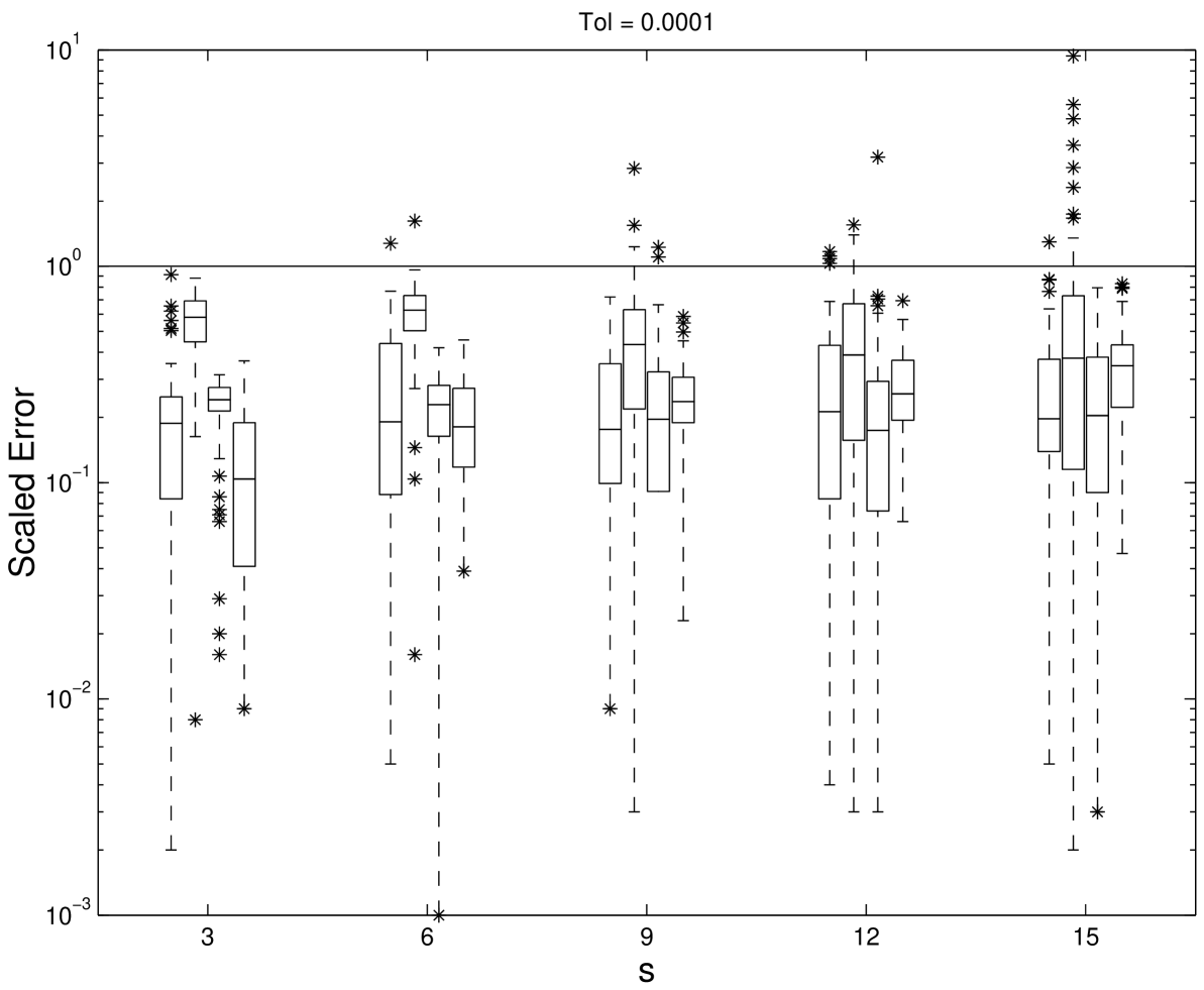
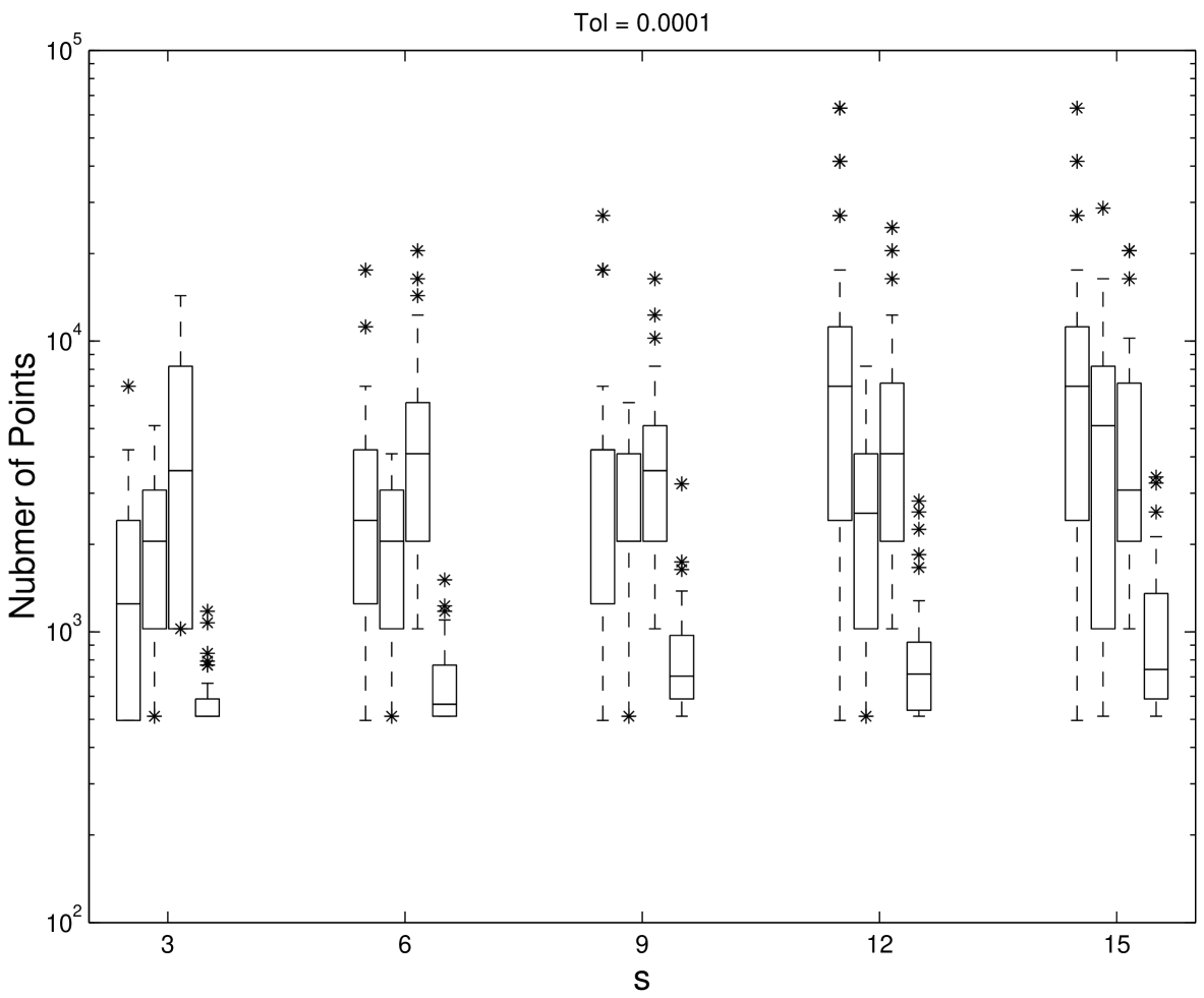
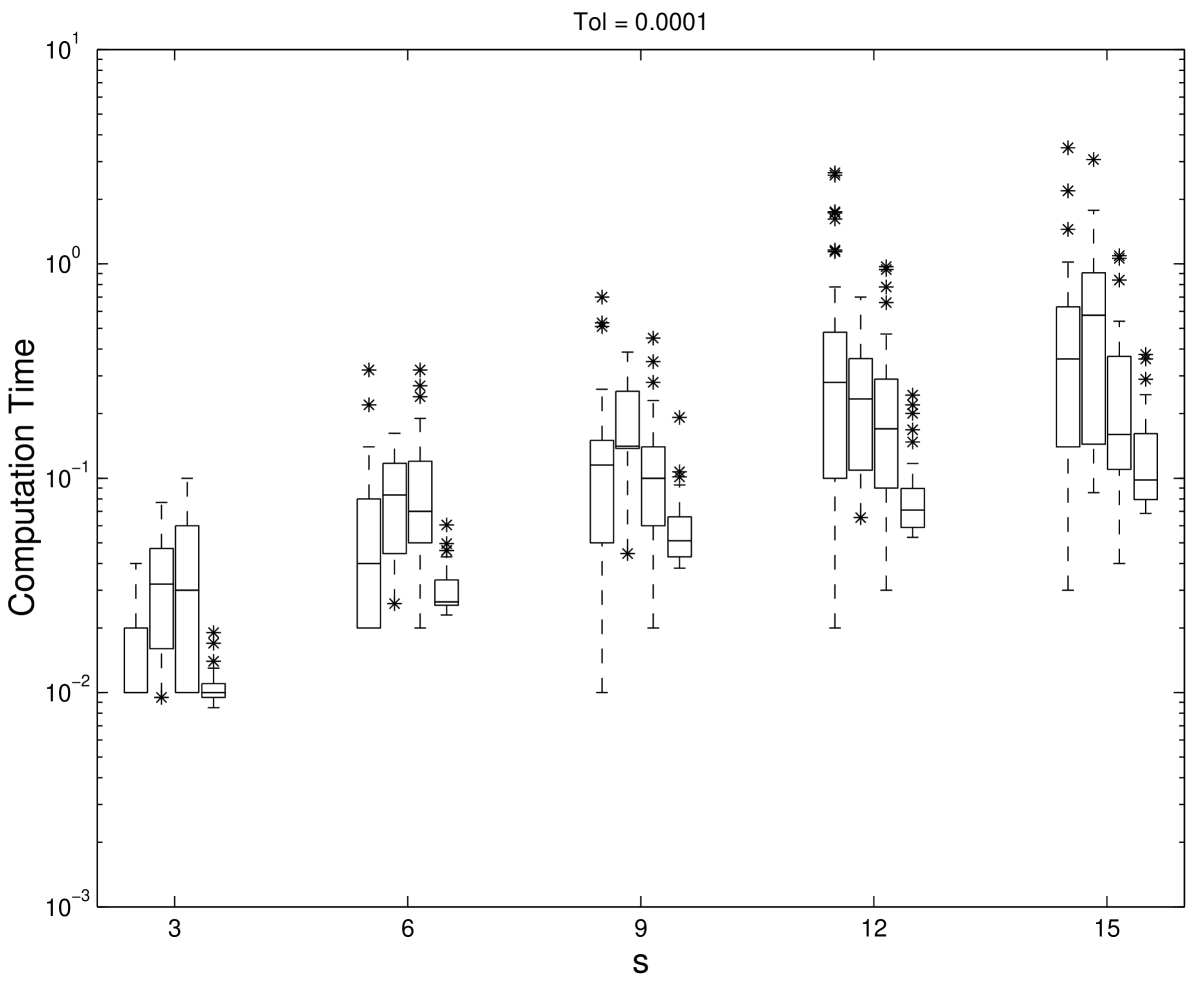
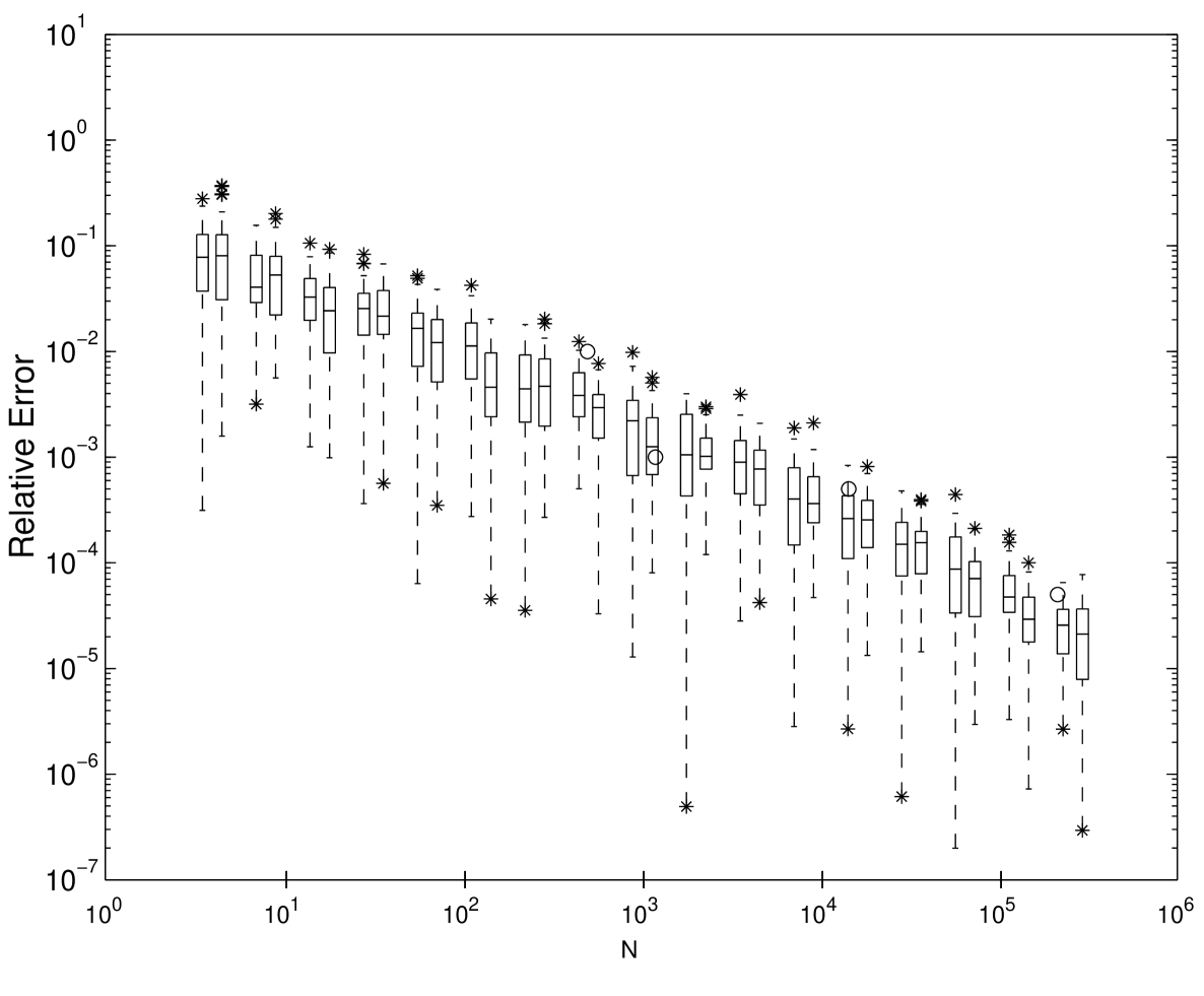
The periodizing transformation , has been applied to the integrand for the second and third algorithms ii. and iii., as it appears to increase the accuracy of these two algorithms. The computations were carried out in Fortran on an Unix workstation in double precision. An absolute error tolerance of was chosen and compared to the absolute error . Error estimation for each algorithm is described in [HHLL01]. Because the true value of the integral is unknown for this test problem, the Korobov algorithm with was used to be “exact” value for computing error. For each , 50 test problems were generated randomly. Figure 5.1, 5.2, and 5.3 show the box and whisker plots of the scaled absolute error , the number of points used, and the computation time in seconds for the four methods with various dimensions. The boxes are divided by the median and contain the middle half of the values. The whiskers show the full range of values and the outliers are plotted as .
The scaled error indicates how conservative the error estimate is. Ideally the scaled error should be close to but not more than one. If the scaled error is greater than one, then the error estimation is not careful enough. However, if the scaled error is much smaller than one, then the algorithm is wasting time by being too conservative. From the Figures 5.1, 5.2 and 5.3 all four methods perform reasonably well in error estimation. The scrambled Sobol’ points, however, use fewer function evaluations and less computation time. Also, their performance is less dependent on the dimension.
5.2 Physics Problem
The following multidimensional integral arising in physics problems is considered by Keister [Kei96]:
| (5.2) |
where denotes the Euclidian norm in , and denotes the standard multivariate Gaussian distribution function. Keister provides an exact formula for the answer and compared the quadrature methods of McNamee and Stenger [MS67] and Genz and Patterson [Gen82, Pat68] for evaluating this integral. Papageorgiou and Traub [PT97] applied the generalized Faure sequence from their FINDER library to this problem. The exact value of the integral is reported in [Kei96, PT97].
Since the methods of McNamee and Stenger and Genz and Patterson performed much worse than FINDER’s generalized Faure sequence, they are ignored here. Instead we compare the scrambled Sobol’ sequences implemented here to the performance of FINDER and the extensible lattice rules described before. To be consistent with the results reported in [PT97] the relative error is computed as a function of . Figure 5.4 shows the results of the numerical experiments for dimension . Box and Whisker plots show how well 50 randomized nets and lattice rules perform. The three algorithms appear to be quite competitive to each other. In some cases randomized Sobol’ performs better than the other two sequences.
5.3 Multidimensional Integration
Consider the following multidimensional integration problem:
| (5.3) |
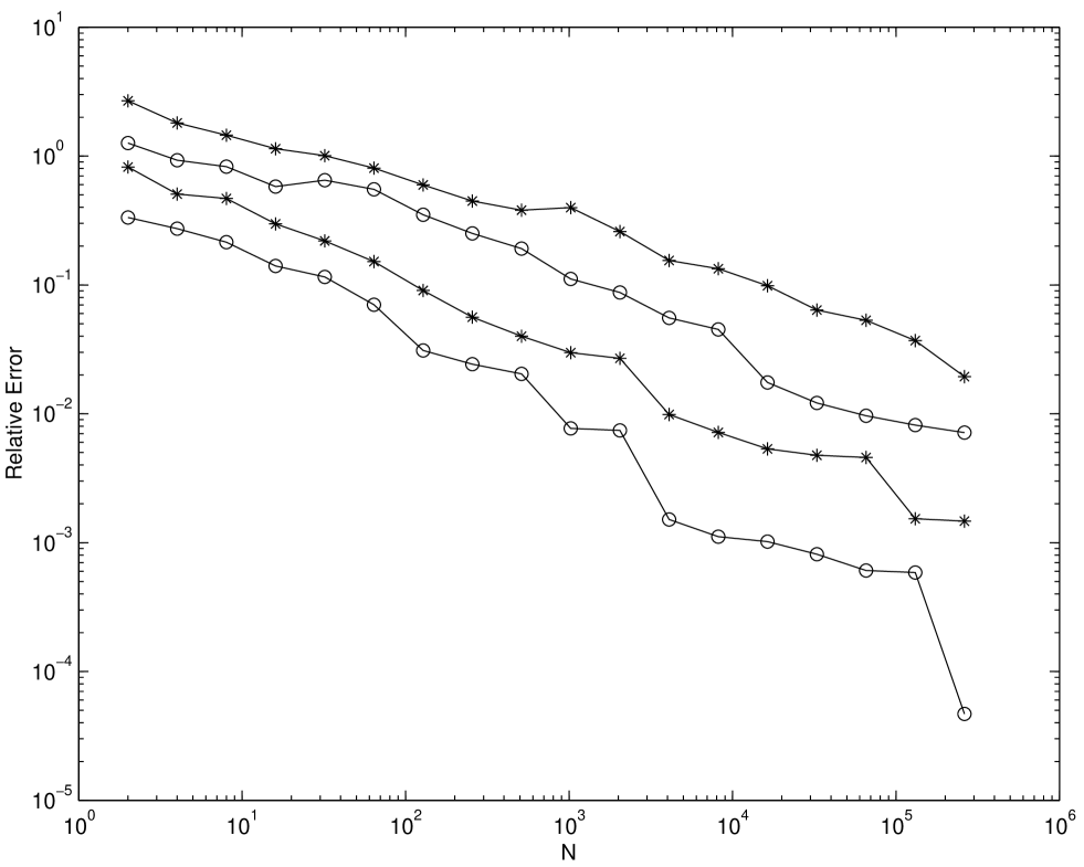
where the exact value of the integration is 1. We numerically compute this problem for the case where with scrambled Sobol’ and EC nets. Figure 5.5 show the root mean square relative error of (5.3) for the scrambled Sobol’ and scrambled EC nets. Figure 5.5 plots the root mean square relative error computed as a function of for and . For scrambling 100 different replications are made. Figure 5.5 shows that the scrambled EC sequence has smaller relative error than the scrambled Sobol’ sequence for all choices of .
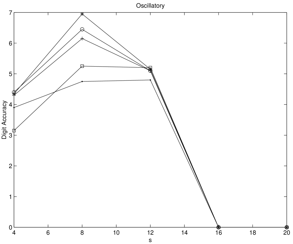
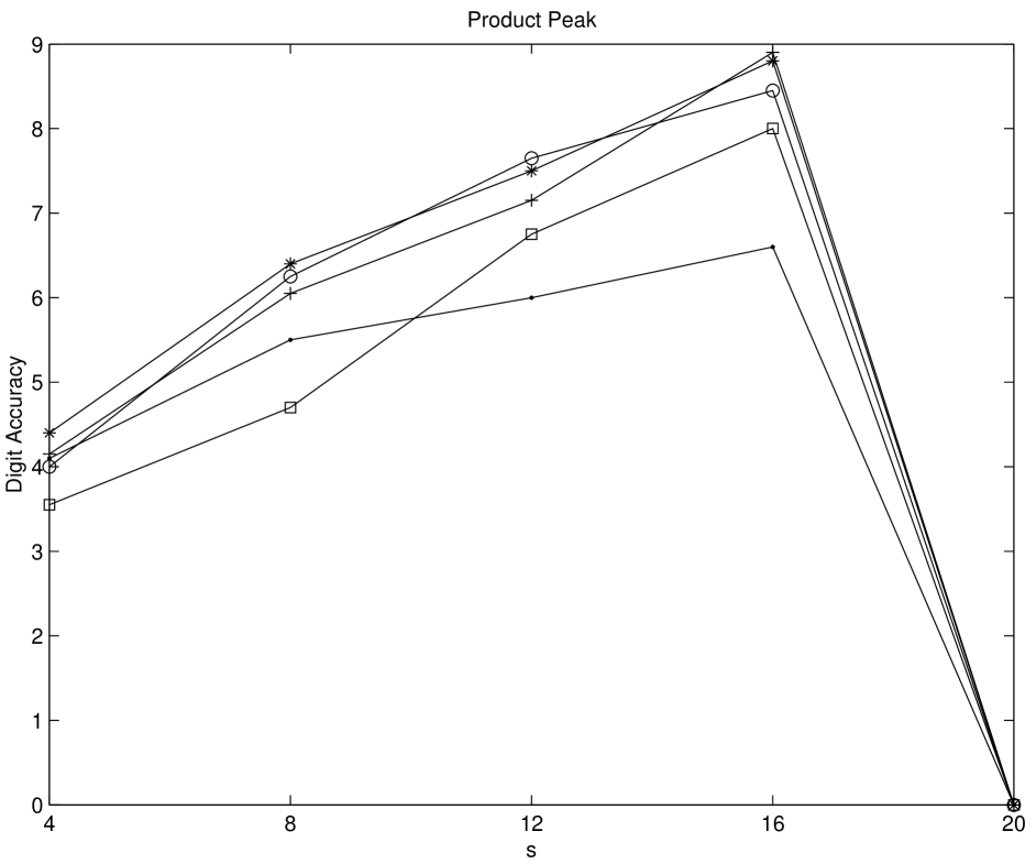
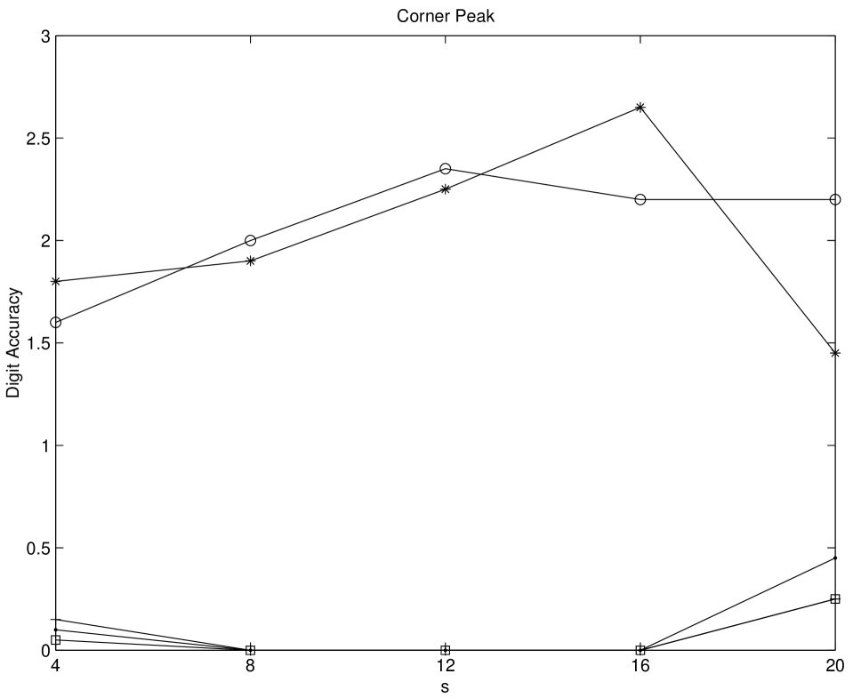
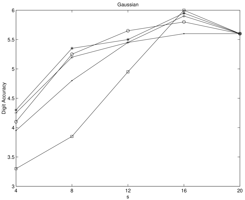
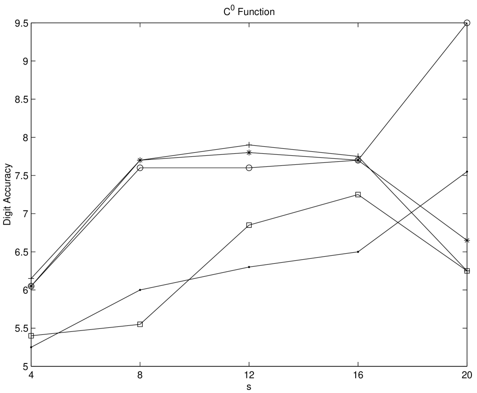
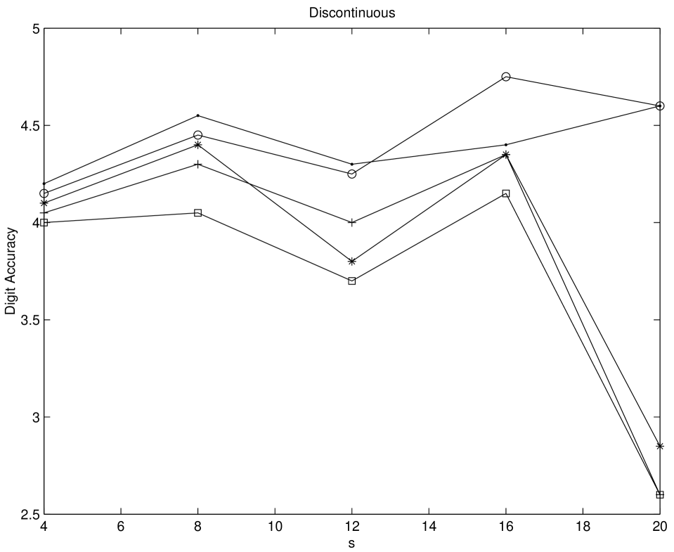
Numerical experiments on multidimensional integrations are performed by using Genz’ test function package [Gen87]. We test his six integral families, namely Oscillatory, Product Peak, Corner Peak, Gaussian, function, and Discontinuous for five different sequences. The compared sequences are Niederreiter-Xing, scrambled Niederreiter-Xing, EC, scrambled EC, and imbedded Niederreiter-Xing sequences. For imbedded Niederreiter-Xing sequence which we choose the generator matrices “nxs20m30”. The choices of parameters are made as in [Gen87]. For scrambled sequences, 20 different replications are performed. The digit accuracy is obtained by computing max(log(relative error),0)). Therefore if the digit accuracy is zero then the relative error is greater than 1. The larger value of the digit accuracy implies the better performance. From Figures 5.6-5.11 it is shown that scrambled nets perform almost always the best. Considering non-scrambled sequences the EC sequence shows the better performance as the dimension of the problem increases. The Niederreiter-Xing sequence tends to perform well in lower dimension, and the imbedded Niederreiter-Xing sequence always performs worse than the Niederreiter-Xing sequence. This is expected because the Niederreiter-Xing sequence are not designed as imbedded sequences. We also test the problems with Sobol’ and scrambled Sobol’ sequences. The performances of Sobol’ and EC sequences are nearly the same.
Chapter 6 Conclusion
In Chapter 2 the randomization of Owen and of Faure and Tezuka have been implemented for the best known digital -sequences. Both types of randomization involve multiplying the original generator matrices by randomly chosen matrices and adding random digital shifts. Base 2 sequences can be generated faster by taking the advantage of the computer’s binary arithmetic system. Using a gray code also speeds up the generation process. The cost of producing a scrambled sequence is about twice the cost of producing a non-scrambled one.
Scrambled sequences often have smaller discrepancies than their non-scrambled counterparts. Moreover, random scrambling facilitates error estimation. On test problems taken from the literature scrambled digital sequences performed as well as or better than other quadrature methods (see Chapter 5).
In Chapter 3 the empirical distribution of the square discrepancy of scrambled digital nets has been fit to a mixture of chi-square random variables as suggested by the central limit theorem by Loh [Loh01]. Apart from some technical difficulties that have been discussed there is a good fit between the empirical and theoretical distributions. Although the digital scrambling schemes used in [Mat98, HH01, YH02] gives the same mean square discrepancy as Owen’s original scheme, the distribution of the mean square discrepancies varies somewhat. It seems that the square discrepancy has a smaller variance for Owen’s scheme. It is shown how one may study the uniformity of lower dimensional projections of sets of points by decomposing the square discrepancy into pieces, . In particular, Sobol’ nets seem to have better uniformity for low dimensional projections than the more recent Niederreiter-Xing nets.
In Chapter 4 new digital -nets are generated by using the evolutionary computation method. The new net shows better equidistribution properties for large and compared to the the Sobol’ sequence. We also compare the exact quality parameters of the new nets with the Niederreiter-Xing nets, where we consider the Niederreiter-Xing nets as an imbedded net. It is shown that the new net has overall smaller values for different dimensional projections. For the and , the new net has better values than the Niederreiter-Xing net in some for . By testing the new nets with multidimensional integration problems, we find that the new nets performs better than Sobol’ and Niederreiter-Xing nets for certain problems. Chapter 5 shows some promising results that it is possible to improve existing nets by the optimization method.
Bibliography
- [AS64] M. Abramowitz and I. A. Stegun, editors. Handbook of Mathematical Functions with Formulas, Graphs and Mathematical Tables. U. S. Government Printing Office, Washington, DC, 1964.
- [BF88] P. Bratley and B. L. Fox. Algorithm 659: Implementing Sobol’s quasirandom sequence generator. ACM Trans. Math. Software, 14:88–100, 1988.
- [BFN92] P. Bratley, B. L. Fox, and H. Niederreiter. Implementation and tests of low-discrepancy sequences. ACM Trans. Model. Comput. Simul., 2:195–213, 1992.
- [CLM+99] A. T. Calyman, K. M. Lawrence, G. L. Mullen, H. Niederreiter, and N. J. A. Sloane. Updated tables of parameters of -nets. J. Comb. Designs, 7:381–393, 1999.
- [CM96] R. E. Caflisch and W. Morokoff. Valuation of mortgage backed securities using the quasi-Monte Carlo method. In International Association of Financial Engineers First Annual Computational Finance Conference, 1996.
- [CP76] R. Cranley and T. N. L. Patterson. Randomization of number theoretic methods for multiple integration. SIAM J. Numer. Anal., 13:904–914, 1976.
- [Fan80] K. T. Fang. Experimental design by uniform distribution. Acta Math. Appl. Sinica, 3:363–372, 1980.
- [Fau82] H. Faure. Discrépance de suites associées à un système de numération (en dimension ). Acta Arith., 41:337–351, 1982.
- [FHN00] K. T. Fang, F. J. Hickernell, and H. Niederreiter, editors. Monte Carlo and Quasi-Monte Carlo Methods 2000. Springer-Verlag, Berlin, 2000.
- [Fog95] D. B. Fogel, editor. Evolutionary Computation:Toward a New Philosophy of Machine Intelligence. IEEE Press, Piscataway, NJ, 1995.
- [Fox99] B. L. Fox. Strategies for Quasi-Monte Carlo. Kluwer Academic Publishers, Boston, 1999.
- [FT00] H. Faure and S. Tezuka. Another random scrambling of digital -sequences. In Fang et al. [FHN00], pages 242–256.
- [Gen82] A. Genz. A Lagrange extrpolation algorithm for sequences of approximations to multiple integrals. SIAM J. Sci. Stat. Comput., 3:160–172, 1982.
- [Gen87] A. Genz. A package for testing multiple integration subroutines. In P. Keast and G. Fairweather, editors, Numerical Integration: Recent Developments, Software and Applications, pages 337–340. D. Reidel Publishing, Dordrecht, 1987.
- [Gen92] A. Genz. Numerical computation of multivariate normal probabilities. J. Comput. Graph. Statist., 1:141–150, 1992.
- [Gen93] A. Genz. Comparison of methods for the computation of multivariate normal probabilities. Computing Science and Statistics, 25:400–405, 1993.
- [Gol89] D. E. Goldberg, editor. Genetic Algorithmsin Search, Optimization and Machine Learning. Addison-Wesley, 1989.
- [Hei00] J. Heitkötter. http://www.cs.bham.ac.uk/mirrors/ftp.de.uu.net/ec/clife/ www/.
- [HH97] F. J. Hickernell and H. S. Hong. Computing multivariate normal probabilities using rank-1 lattice sequences. In G. H. Golub, S. H. Lui, F. T. Luk, and R. J. Plemmons, editors, Proceedings of the Workshop on Scientific Computing, pages 209–215, Hong Kong, 1997. Springer-Verlag, Singapore.
- [HH99] F. J. Hickernell and H. S. Hong. The asymptotic efficiency of randomized nets for quadrature. Math. Comp., 68:767–791, 1999.
- [HH01] H. S. Hong and F. J. Hickernell. Implementing scrambled digital nets. Workshop on the Complexity of Multivariate Problems, October 4–8, 1999, Hong Kong, 2001. submitted to ACM TOMS.
- [HHLL01] F. J. Hickernell, H. S. Hong, P. L’Écuyer, and C. Lemieux. Extensible lattice sequences for quasi-Monte Carlo quadrature. SIAM J. Sci. Comput., 22:1117–1138, 2001.
- [Hic96] F. J. Hickernell. The mean square discrepancy of randomized nets. ACM Trans. Model. Comput. Simul., 6:274–296, 1996.
- [Hic98] F. J. Hickernell. A generalized discrepancy and quadrature error bound. Math. Comp., 67:299–322, 1998.
- [Hic99] F. J. Hickernell. What affects the accuracy of quasi-Monte Carlo quadrature? In Niederreiter and Spanier [NS99], pages 16–55.
- [HL98] P. Hellekalek and G. Larcher, editors. Random and Quasi-Random Point Sets, volume 138 of Lecture Notes in Statistics. Springer-Verlag, New York, 1998.
- [HW01] F. J. Hickernell and H. Woźniakowski. The price of pessimism for multidimensional quadrature. J. Complexity, 17:625–659, 2001.
- [HY01] F. J. Hickernell and R. X. Yue. The mean square discrepancy of scrambled -sequences. SIAM J. Numer. Anal., 38:1089–1112, 2001.
- [Kei96] B. D. Keister. Multidimensional quadrature algorithms. Computers in Physics, 10:119–122, 1996.
- [Kor59] N. M. Korobov. The approximate computation of multiple integrals. Dokl. Akad. Nauk. SSR, 124:1207–1210, 1959. (Russian).
- [Kur92] F. Kursawe, editor. Evolutionary Strategies for Vector Optimization. National Chiao Tung University, Taipei, 1992.
- [Lar98a] G. Larcher. Digital point sets: Analysis and applications. In Hellekalek and Larcher [HL98], pages 167–222.
- [Lar98b] G. Larcher. On the distribution of digital sequences. In H. Niederreiter, P. Hellekalek, G. Larcher, and P. Zinterhof, editors, Monte Carlo and quasi-Monte Carlo methods 1996, volume 127 of Lecture Notes in Statistics, pages 109–123. Springer-Verlag, New York, 1998.
- [Lic98] J. Lichtner. Iterating an -ary gray code. SIAM J. Discrete Math., 11(3):381–386, 1998.
- [Loh01] W. L. Loh. On the asymptotic distribution of scrambled net quadrature, 2001. submitted for publication.
- [Mat98] J. Matousek. On the -discrepancy for anchored boxes. J. Complexity, 14:527–556, 1998.
- [MS67] J. McNamee and F. Stenger. Construction of fully symmetric numerical integration formulas. Numer. Math., 10:327–344, 1967.
- [Nie87] H. Niederreiter. Point sets and sequences with small discrepancy. Monatsh. Math., 104:273–337, 1987.
- [Nie88] H. Niederreiter. Low discrepancy and low dispersion sequences. J. Number Theory, 30:51–70, 1988.
- [Nie92] H. Niederreiter. Random Number Generation and Quasi-Monte Carlo Methods. CBMS-NSF Regional Conference Series in Applied Mathematics. SIAM, Philadelphia, 1992.
- [Nie95] H. Niederreiter. New developments in uniform pseudorandom number and vector generation. In Niederreiter and Shiue [NS95], pages 87–120.
- [Nie99] H. Niederreiter. Constructions of -nets. In Niederreiter and Spanier [NS99], pages 70–85.
- [NS95] H. Niederreiter and P. J.-S. Shiue, editors. Monte Carlo and Quasi-Monte Carlo Methods in Scientific Computing, volume 106 of Lecture Notes in Statistics. Springer-Verlag, New York, 1995.
- [NS99] H. Niederreiter and J. Spanier, editors. Monte Carlo and Quasi-Monte Carlo Methods 1998. Springer-Verlag, Berlin, 1999.
- [NX96] H. Niederreiter and C. Xing. Quasirandom points and global function fields. In S. Cohen and H. Niederreiter, editors, Finite Fields and Applications, number 233 in London Math. Society Lecture Note Series, pages 269–296. Cambridge University Press, 1996.
- [NX98] H. Niederreiter and C. Xing. Nets, -sequences and algebraic geometry. In Hellekalek and Larcher [HL98], pages 267–302.
- [Owe95] A. B. Owen. Randomly permuted -nets and -sequences. In Niederreiter and Shiue [NS95], pages 299–317.
- [Owe97a] A. B. Owen. Monte Carlo variance of scrambled equidistribution quadrature. SIAM J. Numer. Anal., 34:1884–1910, 1997.
- [Owe97b] A. B. Owen. Scrambled net variance for integrals of smooth functions. Ann. Stat., 25:1541–1562, 1997.
- [Owe98] A. B. Owen. Scrambling Sobol’ and Niederreiter-Xing points. J. Complexity, 14:466–489, 1998.
- [Owe99] A. B. Owen. Monte Carlo, quasi-Monte Carlo, and randomized quasi-Monte Carlo. In Niederreiter and Spanier [NS99], pages 86–97.
- [Pat68] T. N. L. Patterson. The optimum addition of points to quadrature formulae. Math. Comp., 22:847–856, 1968.
- [Pir02] G. Pirsic. http://www.dismat.oeaw.ac.at/pirs/niedxing.html, 02.
- [Pir00] G. Pirsic. A software implementation of niederreiter-xing sequences. In Fang et al. [FHN00], pages 434–445.
- [PT96] A. Papageorgiou and J. F. Traub. Beating Monte Carlo. Risk, 9(6):63–65, 1996.
- [PT97] A. Papageorgiou and J. F. Traub. Faster evaluation of multidimensional integrals. Computers in Physics, 11:574–578, 1997.
- [Sch99a] W. Ch. Schmid. The exact quality parameter of nets derived from sobol’ and niederreiter sequences. In eds O. Illiev et al., editor, Recent Advances in Numerical Methods and Applications, pages 287-295. World Scientific, 1999.
- [Sch99b] W. Ch. Schmid. Improvements and extensions of the ”salzburg tables” by using irreducible polymomials. In Niederreiter and Spanier [NS99], pages 476–447.
- [SJ94] I. H. Sloan and S. Joe. Lattice Methods for Multiple Integration. Oxford University Press, Oxford, 1994.
- [Slo85] I. H. Sloan. Lattice methods for multiple integration. J. Comput. Appl. Math., 12 & 13:131–143, 1985.
- [Sob67] I. M. Sobol’. The distribution of points in a cube and the approximate evaluation of integrals. U.S.S.R. Comput. Math. and Math. Phys., 7:86–112, 1967.
- [Tez95] S. Tezuka. Uniform Random Numbers: Theory and Practice. Kluwer Academic Publishers, Boston, 1995.
- [Wah90] G. Wahba. Spline Models for Observational Data. SIAM, Philadelphia, 1990.
- [YH02] R. X. Yue and F. J. Hickernell. The discrepancy and gain coefficients of scrambled digital nets. J. Complexity, 18:135–151, 2002. to appear.
- [YM99] R. X. Yue and S. S. Mao. On the variance of quadrature over scrambled nets and sequences. Statist. Probab. Lett., 44:267–280, 1999.
- [Yue99] R. X. Yue. Variance of quadrature over scrambled unions of nets. Statist. Sinica, 9:451–473, 1999.