Dimension theory of Non-Autonomous iterated function systems
Abstract.
In the paper, we define a class of new fractals named “non-autonomous attractors”, which are the generalization of classic Moran sets and attractors of iterated function systems. Simply to say, we replace the similarity mappings by contractive mappings and remove the separation assumption in Moran structure. We give the dimension estimate for non-autonomous attractors.
Furthermore, we study a class of non-autonomous attractors, named “ non-autonomous affine sets or affine sets”, where the contractions are restricted to affine mappings. To study the dimension theory of such fractals, we define two critical values and , and the upper box-counting dimensions and Hausdorff dimensions of non-autonomous affine sets are bounded above by and , respectively. Unlike self-affine fractals where , we always have that , and the inequality may strictly hold.
Under certain conditions, we obtain that the upper box-counting dimensions and Hausdorff dimensions of non-autonomous affine sets may equal to and , respectively. In particular, we study non-autonomous affine sets with random translations, and the Hausdorff dimensions of such sets equal to almost surely.
1. Introduction
1.1. Self-affine sets
Let be a finite set of affine contractions on with and
| (1.1) |
where is a translation vector, and is a linear transformation on . The set is called a self-affine iterated function system. By the well-known theorem of Hutchinson, see [4, 19], the IFS has a unique attractor, that is a unique non-empty compact such that
| (1.2) |
which is called a self-affine set. If the affine transformations are similarity mappings, we call a self- similar set, see [4] for details.
Formulae giving the Hausdorff and box-counting dimensions of self-similar sets satisfying the open set condition are well-known, see [4]. However, calculation of the dimensions of self-affine sets is more awkward, see [2, 9, 12, 15, 22, 25]. For each , we write for the set of words of length . Let be the singular value function defined by (2.14). Falconer in [5] defined the criticla value which is the unique solution to
and it is often called affine dimension or Falconer dimension. Given for it turns out that
| (1.3) |
for almost all (in the sense of -dimensional Lebesgue measure), we refer the readers to [5, 27] for details. Note that is always the upper bound for the box-counting dimension of self-affine sets, Falconer in [6] proved that the box-counting dimension and affine dimension coincide by applying projection condition with other assumptions. From then on, a considerable amount of literature has been published on the validation of formula (1.3) under various conditions. In particular, in [20], Jordan, Pollicott and Simon studied perturbed self-affine sets where they changed translations into independently identically distributed random variables, and they showed that for , the dimension formula (1.3) holds almost surely. In [10], Falconer and Kempton showed the dimension formula (1.3) holds for all translations in under various assumptions. We refer readers to [1, 6, 7, 8, 11, 13, 14, 16, 18, 24] for various related studies.
1.2. Moran sets
Moran sets were first studied by Moran in [23], and we recall the definition for the readers’ convenience.
Let be a sequence of integers greater than or equal to . For each , we write
| (1.4) |
for the set of words of length , with containing only the empty word , and write
| (1.5) |
for the set of all finite words.
Suppose that is a compact set with (we always write int( for the interior of a set). Let be a sequence of positive real vectors where for each . We say the collection of closed subsets of fulfils the Moran structure if it satisfies the following Moran structure conditions (MSC):
-
(1).
For each , is geometrically similar to , i.e., there exists a similarity such that . We write for the empty word .
-
(2).
For all and , the elements of are the subsets of with disjoint interiors, ie., for . Moreover, for all ,
where denotes the diameter.
The non-empty compact set
is called a Moran set determined by . For each , the element is called a th-level basic set of . For each integer let be the unique real solution of the equation
| (1.6) |
Let and be the real numbers given respectively by
| (1.7) |
It was shown in [17, 28, 29] that if the following dimension formulae hold
The dimension theory of Moran sets has been studied extensively, and we refer the readers to [17, 28, 29] for detail and references therein. Note that, in the definition of Moran sets, the position of in is very flexible, and the contraction ratios may also vary at each level. Therefore the structures of Moran sets are more complex than self-similar sets, and in general, the inequality
holds strictly for Moran fractals. The general lower box dimension formula for Moran sets is still an open question. Except providing various examples, Moran sets are also useful tools for analysing properties of fractal sets in various studies, for example, see [28] and references therein for applications.
Note that similarities and separation assumption are required in the Moran structure, Inspired by the structure of iterated function systems, we generalize the Moran structure to non-autonomous structure where we replace similarities by contractions or affine mappings, and remove the separation assumption. The geometric properties of non-autonomous sets are more complex than Moran sets since mappings may have different contraction ratios in different directions. Therefore, non-autonomous sets provide not only interesting phenomena but also useful tools for fractal analysis. Different to the attractors of iterated function systems, non-autonomous sets do not have dynamical properties any more, and the tools in ergodic theory cannot be invoked. As a result, it is more difficult to explore their dimension formulae and other fractal properties.
In this paper, we investigate the dimension theory of non-autonomous attractors, and particularly, we are interested in a classs of attractors, named “non-autonomous affine sets or affine sets”. In section 2, we first give the definition of non-autonomous attractors and estimate the dimensions of such sets, then we study the non-autonomous affine sets and state the main conclusions in subsection 2.3. The dimension estimates for non-autonomous sets are provided in section 3. Upper and lower box dimensions of non-autonomous affine sets are explored in section 4. We discuss the upper bounds of Hausdorff dimensions of non-autonomous affine sets in section 5, and we give the Hausdorff dimension formula for a spectial class of non-autonomous affine sets with finitely many translations. In section 6, we study the Hausdorff dimension of non-autonomous affine sets with random translations, and we prove that with probability one, the Hausdorff dimensions of such sets equal to a critical value. Finally, in section 7, we compare critical values of non-autonomous affine sets, and we also provide some examples to illustrate our conclusions.
2. Non-autonomous iterated function systems
2.1. Definition of non-autonomous iterated function systems
Let be a sequence of integers such that for all . Let and be given by (1.4) and (1.5), respectively. Suppose that is a compact set with non-empty interior. Let be a sequence of collections of contractive mappings, that is
| (2.8) |
where each satisfies that for some . We say the collection of closed subsets of fulfils the non-autonomous structure with respect to if it satisfies the following conditions:
-
(1).
For all integers and all , the elements of are the subsets of . We write for the empty word .
-
(2).
For each , there exists an transformation such that
where , for some , and , .
-
(3).
The maximum of the diameters of tends to 0 as tends to , that is,
We call a non-autonomous iterated function systems(NIFS) determined by , and the non-empty compact set
| (2.9) |
is called a non-autonomous attractor determined by . For all , the elements are called th-level basic sets of . If the non-autonomous attractor satisfies that for all integers and ,
we say satisfies Moran separation condition (MSC).
Remark (1) Overlap is allowed in the structure, and Moran sets are special non-autonomous attractors satisfying Moran separation condition. Note that Moran sets are always uncountable, but the cardinality of non-autonomous attractors sets may be finite, countable or uncountable even if Moran separation condition is satisfied, see Example 2 and Example 3 in section 7.
(2) In the definition, the transformation may be determined in the following way. For each and , there exists an mapping such that
Suppose that for each and , the affine mapping is defined. For each and , there exists an affine mapping such that
(3) The assumption in the definition is necessary, otherwise the set may have positive finite Lebesgue measure, and we do not consider such case in this paper, see Example 1 in section 7.
(4) Non-autonomous iterated function system is also a generalization of the iterated function system. However, for , the transformations and in and have the same contractive part but with different translations. Therefore the non-autonomous attractor may be different to the attractor of classic iterated function system even if the sequence is identical, that is, and for all .
For general non-autonomous sets, it is difficult to find their fractal dimensions, but we are still able to provide some rough estimates if contraction ratios are known.
Theorem 2.1.
We next obtain a lower bound for Hausdorff and box-counting dimensions in the case where the basic sets of satisfy the following condition. We say the non-autonomous set satisfies gap separation condition(GSC) if there exists a constant such that for all , , we have that
Theorem 2.2.
Note that if the contractions are all similarities in the NIFS , then is frequently used to guarranttee the lower bounds in Theorem 2.2. For general NIFSs, is not sufficient for the theorem, see Example 3 for a counterexample.
To study the dimension properties of non-autonomous sets, the following notations are frequently used in our context. Let and be given by (1.4) and (1.5), respectively. Let be the corresponding set of infinite words, where is the sequence of integers.
For , we write and write for the length of . For each , and , we say is a curtailment of , denote by , if . We call the set the cylinder of , where . If , its cylinder is .
For , let denote the maximal common initial finite word of both and . We topologise using the metric for distinct to make a compact metric space. The cylinders for form a base of open and closed neighbourhoods for . We call a set of finite words a covering set for if .
For , we denote compositions of mappings by . Let be the projection given by
It is clear that the attractor is the image of , i.e. . Note that the projection is surjective. To emphasize the dependence on translations, we sometimes write and instead of and .
Let be a finite Borel regular measure on . We define , the projection of the measure onto , by
| (2.11) |
for , or equivalently by
| (2.12) |
for every continuous . Then is a Borel measure supported by .
2.2. Non-autonomous affine iterated function systems
Let be a sequence of collections of contractive matrices, that is
| (2.13) |
where are matrices with for . The collection of closed subsets of fulfils the non-autonomous structure with respect to the sequence of contractive matrices. We call the non-autonomous affine iterated function system (NAIFS) determined by , and we call the attractor given by (2.9) a non-autonomous affine set(NAS) or affine set determined by .
Note that Moran sets may be regarded as a special case of non-autonomous affine sets satisfying Moran separation condition, where is the multiplication of contraction ratio and a rotation matrix .
Let be a contracting and non-singular linear mapping. The singular values , of are the lengths of the (mutually perpendicular) principle semi-axes of , where is the unit ball in . Equivalently they are the positive square roots of the eigenvalues of , where is the transpose of . Conventionally, we write that .
For , the singular value function of is defined by
| (2.14) |
where is the integer such that . For technical convenience, we set for . It is clear that is continuous and strictly decreasing in . The singular value function is submultiplicative, that is, for all ,
| (2.15) |
for all , see [5] for details.
Let be given by (2.13). We write
| (2.16) | |||||
Immediately, for each , the singular value function of is bounded by
| (2.17) |
Note that for a self-affine set , the sequence is submultiplicative, and this implies that the function
is continuous and strictly decreasing in . This property plays an important role in finding the affine dimensions of self-affine fractals. However, in general, the submultiplicative property does not hold for non-autonomous affine sets. The lack of submultiplicativity causes one of the main difficulties to determine the dimensions of non-autonomous affine sets.
2.3. Main conclusions for non-autonomous affine sets
Given . Let be the NAIFS (2.13) and be the corresponding non-autonomous affine set defined by(2.9). From now on, we always assume that the matrices in for all are nonsingular, and
| (2.18) |
For each and , let be the integer such that and define
The set is a cut-set or stopping in the sense that for every , there is a unique integer such that . For each , by (2.15) and (2.16), we have that
We define
| (2.19) |
The critical value plays a key role in the box dimensions of non-autonomous affine sets. The following theorem shows that is an upper bound for the upper box dimension of .
Theorem 2.3.
Let be the non-autonomous affine set given by (2.9). Then
Suppose that the matrices in for all are scalar matrices, that is is a scalar matrix for each and each . Suppose that satisfies the MSC. Then is a Moran set, and gives the upper box dimension.
Corollary 2.4.
Next we show that under certain strong restrictions, the critical value gives the upper box dimension of . We say the non-autonomous affine set satisfies the open projection condition(OPC) if there exists an open set such that and for each and ,
with the union disjoint, and
for all -dimensional subspaces .
Theorem 2.5.
Let be the non-autonomous affine set given by (2.9) and satisfying OPC. Suppose that there exists such that
for all -dimensional subspaces and all . Then
For self-affine fractals, the box-counting dimensions and Hausdorff dimensions are bounded by the same value . Unfortunately, does not provide much information for the Hausdorff dimensions of non-autonomous affine sets, and we have to find a different candidate for Hausdorff dimensions.
Fix . By applying “Method II” in Rogers [26], we define a Hausdorff type measure on as follows. For each integer , let
We obtain a net measure of Hausdorff type by letting
| (2.20) |
for all . Note that is an outer measure which restricts to a measure on the Borel subsets of .
We define
| (2.21) |
The critical value is important in studying the Hausdorff dimensions for non-autonomous affine sets. The following theorem shows that is an upper bound for the Hausdorff dimension of .
Theorem 2.6.
Let be the non-autonomous affine set given by (2.9). Then
In section 7, we discuss the relations of , and , and we also give some examples to show that and are sharp bounds for Hausdorff dimensions and upper box dimensions of non-autonomous affine sets, respectively, see Example 4 in section 7.
Given the discontinuity of dimensions of in the translations , we can only expect to show that is also a lower bound for Hausdorff dimensions for almost all constructions, in some sense.
First, we consider a special case where the translations of affine mappings in the non-autonomous structure are selected only from a finite set. Let be a finite collection of translations, where are regarded later as variables in . For each , we have that . Suppose that the translation of is an element of , that is,
for . We write as a variable in . To emphasize the dependence on these special translations in , we denote the non-autonomous affine set by . The following conclusion shows that the Hausdorff dimension of equals almost surely.
Theorem 2.7.
Given . Let be the non-autonomous affine set given by (2.9) where the translations of affine mappings are chosen from . Suppose that
Then for -almost all ,
if ,
if .
As you can see the set is special and unnatural, the reason is that there is no obvious candidate which would take the place of the Lebesgue measure in infinite dimensional spaces. Inspired by [8, 20], we study the Hausdorff dimensions of non-autonomous affine sets in probabilistic language.
Let be a bounded region in . For each , let be a random vector distributed according to some Borel probability measure that is absolutely continuous with respect to -dimensional Lebesgue measure. We assume that the are independent identically distributed random vectors. Let denote the product probability measure on the family In this context, for each , we assume that the translation of is an element of , that is,
for . We also assume that the collection of fulfils the non-autonomous structure, and we call the non-autonomous affine set with random translations.
Next theorem states that, in this probabilistic setting, the Hausdorff dimension of equals with probability one.
Theorem 2.8.
Let be the non-autonomous affine set with random translation. Then for -almost all ,
if ,
if .
Finally, we explore the lower box-counting dimension of non-autonomous affine sets. Under open projection condition, we show that is a lower bound for the lower box dimension.
Theorem 2.9.
Let be the non-autonomous affine set given by (2.9) with the open projection condition satisfied. Suppose that there exists such that
for all -dimensional subspaces and all . Then
Corollary 2.10.
Let be the non-autonomous affine set in given by (2.9) with the open projection condition satisfied. Suppose that has a connected component which is not contained in any straight line, and for each . Then
3. Dimension estimates of non-autonomous sets
In this section, we estimate the dimensions of the attractor of an NIFS consisting of contractions which are no similarities.
First, we show that the Hausdorff dimension and upper box-counting dimension are upper bounded by and given by (1.7), respectively, if for all ,
where , for all .
Proof of Theorem 2.1.
For , we write and . Since for all ,
for every , it is clear that .
First, we prove that . For , there exits a sequence such that , and it follows that . For , there exists such that , and the set is a -cover of . Hence
By taking , we have . Since is arbitrarily chosen, it follows that .
Next, suppose that , and we prove that .
For each given , there exists such that for , . It follows that . Recall that for . For sufficiently small , let
Then is a -cover of , and . Let denote the cardinality of a set. Thus , and
Fix sufficiently small . Let
where .
For each , it is clear that for all . If , we have that
otherwise for , we write that , and obtain that
By repeating this process, we have
for some . Hence , and it implies . ∎
Next, we show that and given by (1.7) are the lower bounds of Hausdorff dimension and upper box-counting dimension of non-autonomous set , respectively, if satisfies GSC, and for all ,
where , for all .
Proof of Theorem 2.2.
First, we prove that . For each , there exists such that for , , which implies that .
Let , and be a probability Borel measure on defined by
where . Then is a probability Borel measure on .
For each , there is a unique such that for each . Fix , we write
where is the constant in the definition of gap separation condition. Given , there exists such that . Since satisfies gap separation condition, we have that , and it implies that . Hence
For each such that and , we have that for some , and it implies that . By the Mass distribution principle, see [4, Theorem 4.2], we have that . Since is arbitrarily chosen, it follows that .
Next, we prove that . Fix . There exists a sequence of such that , and it implies that
For each large , it is clear that
Let be cardinality of the set . Then there exists such that
and for all , by the gap separation condition, the gap between and is at least
This implies that for every , the ball intersects only one basic set at th level with . Hence , and immediately, we have that
It follows that for all , and the conclusion holds. ∎
4. Box-counting dimensions of non-autonomous affine sets
Recall that for each and , let be the integer that and
For all real such that , we always have that
| (4.22) |
Since for each , is continuous and strictly decreasing, it is clear that
is continuous and strictly decreasing on .
Let be the smallest number of sets with diameters at most covering the set . First we give the proof for that is the upper bound for the upper box dimension of .
Proof of Theorem 2.3.
Let be a ball such that . Given , there exists an integer such that for all . Let be a covering set of such that for each . Then . Each ellipsoid is contained in a rectangular parallelepiped of side lengths where the are the singular values of .
Fix . Let be the least integer greater than or equal to . We divide such a parallelepiped into at most
cubes of side . Hence, the total number of cubes with side covering is bounded by
Since , it is clear that
| (4.23) |
Since we only know that is continuous and strictly decreasing on , we consider the following two cases:
Case (1): Since , there exists a constant such that for ,
| (4.24) |
where is a constant. By (4.23), it follows that
where .Hence
and it implies that
Therefore, the conclusion holds.
Case (2): Suppose that . Let be the least integer greater than , and let be non-integral with . By the definition of , there exists such that and
Since , we have that . Hence for each ,
It follows that
By the similar argument as above, we have that
and it implies that . Since is chosen arbitrarily, we have that
and the conclusion holds.
∎
To prove that is the lower bound of upper box dimension, we need the following technical lemma which gives a sufficient condition for the upper box dimension of .
Lemma 4.1.
Let be the non-autonomous affine set given by (2.9). Suppose that there exists an increasing sequence convergent to and a sequence such that for each integer ,
for all . Then .
Proof.
Since is increasing and convergent to , we assume that is non-integral such that for some integer . By the definition of and , we have that
Hence there exists a sequence such that , and
| (4.25) |
Since
we have that
It follows that
for all . Since , letting tends to infinite, the conclusion holds. ∎
Proof of Corollary 2.4.
Since are scalar matrices, for , the matrix is still a scalar matrix given by
We write
and it is clear that and
Note that is independent of .
Proof of Theorem 2.5.
By Theorem 2.3, it is clear that . If , it is clear that
and the conclusion holds. Hence we only need to show for .
Let be the open set in the OPC condition. Given , we write
For each given -dimensional subspace , by the continuity of Lebesgue measure, it is clear that monotonically increases to as tends to . Since and are continuous in with respect to the Grassmann topology on the set of -dimensional subspaces, by Dini’s theorem, we have that uniformly converges to in . Since , we may choose such that
for all subspaces . Let , then
For each , if is the -dimensional subspace of perpendicular to the shortest semi-axis of the ellipsoid , where is the unit ball in . Let , then
| (4.26) |
for , then there exists such that . Let , then and . Hence
| (4.27) |
for all . For all such that , it is clear that the distance from to the set is no more that. Combining (4.26) and (4.27) together, we obtain that
Arbitrarily choose . For each , the set is independent of . Note that OPC condition implies that is a union of disjoint open sets. For each ,
Note that the set may be covered by balls of radius if is covered by balls of radius . Therefore,
where is the volume of the d-dimensional unit ball. It follows that
By Lemma 4.1, we obtain that , and the conclusion holds. ∎
Next, we prove that is a lower bound for the lower box-dimension of the non-autonomous affine set .
Proof of Theorem 2.9.
Since
for all -dimensional subspaces , the Hausdorff dimension of is at least . By Theorem 2.6, . If , then
Hence it is sufficient to show for s.
For every , we have that . Hence there exists a constant such that for all sufficiently small ,
By the same argument as in Theorem 2.5, we have that
This implies that
where . Using the Minkowski definition of box-counting dimension, see [4], it follows that
for all . Hence , and the conclusion holds. ∎
5. Hausdorff dimension of non-autonomous affine sets
First, we give the proof that is an upper bound for the Hausdorff dimension of non-autonomous affine sets.
Proof of Proposition 2.6.
Let be a sufficiently large ball such that . Given , there exists an integer such that for all such that . Let be a covering set of such that for each . Then . Each ellipsoid is contained in a rectangular parallelepiped of side lengths where the are the singular values of .
For each , let be the least integer greater than or equal to . We can divide such a parallelepiped into at most
cubes of side .
Taking such a cover of each ellipsoid with , it follows that
Since this holds for every covering set with for , we have that
Letting tend to , it follows that
Hence for all , which implies that . ∎
The following cited theorem gives a necessary and sufficient condition for absolute continuity of measures, which is very useful in our proofs, and we refer readers to [21, Theorem 2.12] for details.
Theorem 5.1.
Let and be Radon measures on . Then if and only if
for -almost all .
To show that is also a lower bound for the Hausdorff dimension of non-autonomous affine sets, we need the following lemmas for the connection between integral estimates and singular value functions.
The first lemma shows that singular value functions provide useful estimates for potential integrals, which was proved by Falconer in [5, Lemma 2.1]. Let be the closed ball in with centre at the origin and radius .
Lemma 5.2.
Let satisfy with non-integral. Then there exists such that, for all non-singular linear transformations ,
The next lemma provides a technical result on net measures.
Lemma 5.3.
Let be the Borel measure defined by (2.20). If then there exists a Borel measure on such that and a constant such that
| (5.28) |
for all .
Proof.
Since , by a similar argument to Theorem 5.4 in [3], there exists a compact such that and
for all , where is a constant independent of . (Alternatively, This may be regarded as a special case of Theorem 54 in [26].)
We write for the measure given by
for all Borel , and the measure has the desired properties. ∎
Recall that is a finite collection of translations, where are regarded as variables in . For each , . Suppose that the translation of is an element of , that is,
for . We write as a variable in . To emphasize the dependence on these special translations in , we denote the non-autonomous affine set by and denote the projection by , that is
It is clear that . We write for the closed ball in with centre the origin and radius .
Lemma 5.4.
Let satisfy with non-integral. Suppose that there exists a constant such that, for all , ,
| (5.29) |
Then
for -almost all .
Proof.
Finally, we prove that gives the Hausdorff dimension of non-autonomous affine sets almost surely.
Proof of Theorem 2.7.
Recall that
where . For , we assume that . Without loss of generality, suppose that , . Then
where is a linear map from to . We may write .
We write
and we have that Let
If , it is straightforward that
Otherwise for , it is clear that and can not equal to and simultaneously. We assume that . Since , it follows that
This implies that the linear transformation is invertible. We define the invertible linear transformation by
| (5.31) |
For , arbitrarily choosing a non-integral , by Lemma 5.2 and (5.31), it follows that
Immediately, Lemma 5.4 implies that
for -almost all . Combining Theorem 2.6, the equality
holds for -almost all .
Next, we prove that for . Arbitrarily choose . Then by the definition of , we have that . By Lemma 5.3, there exists a Borel measure on such that and a constant such that
| (5.32) |
for all Let be the projection measure of , that is . It is clear that
To prove that , we just need to prove . By Theorem 5.1, it is equivalent to show that for -almost all ,
For simplicity, we write for the singular values of . For all distinct and , by (5.31), we have that
where is a constant. Applying Fatou’s Lemma and Fubini’s Theorem, this implies that
Furthermore, by (5.32) and (2.17), we have that for ,
| (5.33) |
By the similar argument as above, we have that
Hence for -almost all , the inequality
holds for -almost all . By Theorem 5.1, this implies that . Since , it implies that for -almost all , and the conclusion holds.
∎
6. Affine Moran set with random translations
Recall that is a bounded region in . For each , the translation is an independent random vector identically distributed according to the probability measure which is absolutely continuous with respect to -dimensional Lebesgue measure. The product probability measure on the family is given by
For each , let , where the translation of is an element of , that is,
for . Assume that the collection fulfils the non-autonomous structure. Since
where , j=1,2,3…, are random vectors. The points are random points whose aggregate form the random set , that is,
and is called non-autonomous affine set with random translations.
Let denote expectation. Given , we write for the sigma-field generated by the random vectors for and write for the expectation of a random variable conditional on ; intuitively this is the expectation of given all .
With respect to the probability setting, we have a similar conclusion to Lemma 5.4 to estimate the potential integral. Since the proof is almost identical, we omit it.
Lemma 6.1.
Let satisfy with non-integral. Suppose that there exists such that
for all , , where for any subset of such that and but , where . Then
for almost all .
Finally, we prove that for almost all , the critical value gives the Hausdorff dimension of the non-autonomous affine set .
Proof of Theorem 2.8.
By Theorem 2.6, the critical value is the upper bound to the Hausdorff dimension of , that is, . We only need to show that is also the lower bound.
Fix . Let . Then
where is a random vector which is independent of . Since the measure is absolutely continuous with respect to with bounded density, we have that
For simplicity, we write for the singular values of . Let be the integer such that . Since is a bounded region in , there exists such that . It is clear that
By moving to , we have that
Combining with these two facts, we have that
where and are constants independent of and .
Therefore, for all with non-integral, we obtain that
for all , . By Lemma 6.1, we have that , and the conclusion holds.
We next prove part (2). Choose such that . By the definition of , we have that . By Lemma 5.3, there exists a Borel measure on such that and a constant such that
| (6.34) |
for all Let be the projection measure of given by (2.11). It is clear that
By similar argument as above, for all distinct and , there exist a constant such that
Furthermore, by (6.34) and (2.17), we have that for ,
Hence for -almost all , we obtain that
for -almost all . Since , by Theorem 5.1, it follows that for -almost all , and the conclusion holds. ∎
7. Comparison of critical values and some examples
In this section, we discuss the relations of the critical values , and the affine dimension . The first conclusion follows straightforward from their definitions.
Note that the inequality may hold strictly, see Example 4. Moreover, generally does not exist in non-autonomous affine IFS.
In the following special cases, the two critical values and may coincide with . Remind that the non-autonomous affine set may not be self-affine fractals even if the sequence is identical, see Remark (4) after the definition of non-autonomous affine sets.
Theorem 7.2.
Suppose that and for all . Then
Proof.
Since , we have that for all . This implies that
Thus is a submultiplicative sequence, so by the standard property of such sequences, exists for each . Since for each and ,
we have that is continuous and strictly decreasing in . Since the limit is greater than 1 for and less than 1 for sufficiently large , there exists a unique , written as , such that
First, we show that . For each ,
Hence
It follows that . Then we have .
Next, we show . Let be the integer that . Arbitrarily choosing , then . Thus there exists a covering set of such that
Let . For , we define further covering sets by
Then by the submultiplicativity of ,
Applying this inductively, we obtain that
If , then , where and . Moreover, for such each , there are at most such . Since ,
Since it holds for all , we have that
Hence , and it implies that . By Proposition 7.1, we obtain that
∎
The Hausdorff dimension of self-affine sets immediately follows from Theorem 2.7 and Theorem 7.2, see[5, 27]
Corollary 7.3.
Let be the self-affine set given by (1.2), where . Suppose that for all . Then for -almost all ,
if ,
if .
The Hausdorff dimension of self-affine sets with random translation immediately follows from Theorem 2.8 and Theorem 7.2, see[20]
Corollary 7.4.
Let be the self-affine set with random translation. Then for -almost all ,
if ,
if .
Finally, we give some examples to illustrate the definition of non-autonomous affine sets and our conclusions.
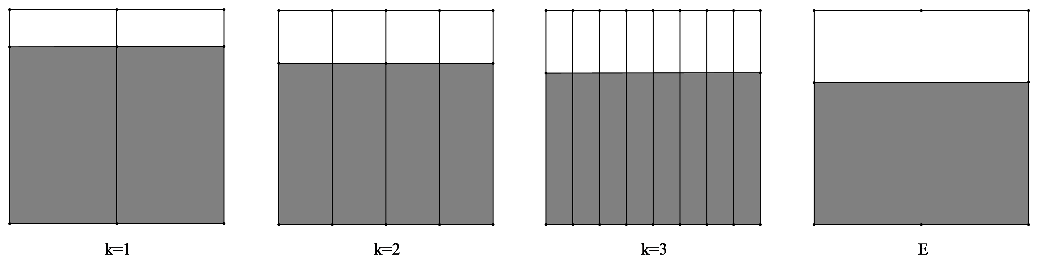
Example 1.
Suppose that and . For all , ,
Then
and has non-empty interior. Hence all dimensions of equals .
Note that Moran sets are always uncountable. In the following examples, we show that non-autonomous affine sets may be finite, countable or uncountable even if the Moran separation condition is satisfied.
Example 2.
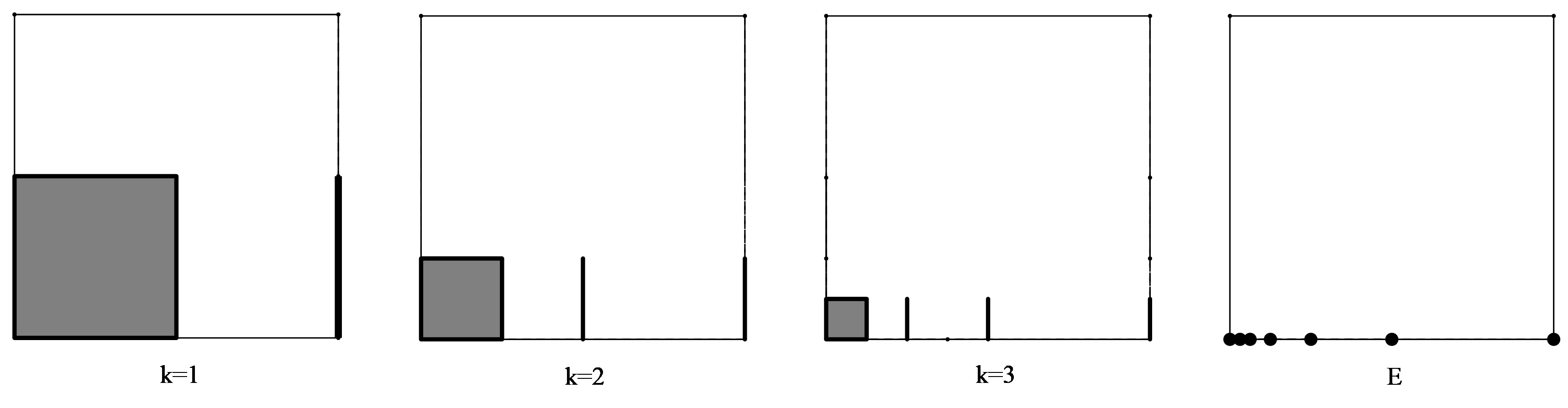
Example 3.
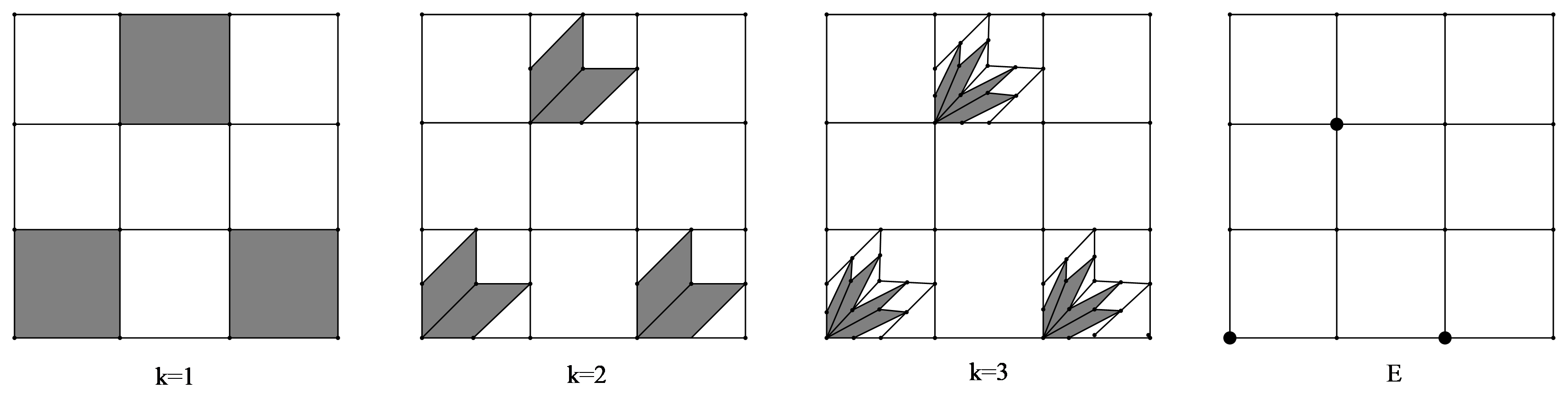
Next, we give an example that and are the sharp bounds for the upper box dimension and the Hausdorff dimension of non-autonomous affine sets.
Example 4.
Suppose that and . For each integer ,
Let and . For , , and
where . Let be the number of such that for some . Suppose that for each , . Then for ,
By simple calculation, we have that
But
and
References
- [1] B. Bárány and M. Hochman and A. Rapaport. Hausdorff dimension of planar self-affine sets and measures. Invent. Math., 216, 601–659, 2019.
- [2] T. Bedford. Crinkly curves, Markov partitions and box dimensions in self-similar sets. PhD thesis, University of Warwick, 1984.
- [3] K. J. Falconer. The Geometry of Fractal Sets. Cambridge University Press, 1985.
- [4] K. J. Falconer. Fractal Geometry-Mathematical Foundations and Applications. John Wiley & Sons Inc., 2nd edt, 2003.
- [5] K. J. Falconer. The Hausdorff dimension of self-affine fractals. Math. Proc. Cambridge Philos. Soc., 103, 339–350, 1988.
- [6] K. J. Falconer. The dimension of self-affine fractals. II. Math. Proc. Cambridge Philos. Soc., 111, 169–179, 1992.
- [7] K. J. Falconer. Generalized dimensions of measures on self-affine sets, Nonlinearity 12, 877–891, 1999.
- [8] K. J. Falconer. Generalized dimensions of measures on almost self-affine sets. Nonlinearity 23, 1047–1069, 2010.
- [9] K. J. Falconer. Dimensions of self-affine sets: a survey. Further developments in fractals and related fields, 115–134, Trends Math., Birkhäuser/Springer, New York, 2013.
- [10] K. J. Falconer and T. Kempton. Planar self-affine sets with equal Hausdorff, box and affinity dimensions. Ergodic Theory Dynam. Systems, 38,1369–1388, 2018.
- [11] D. Feng. Dimension of invariant measures for affine iterated function systems Feng. Duke Math. J. 172, 701–774, 2023.
- [12] D. Feng and H. Hu. Dimension Theory of Iterated Function Systems. Comm. Pure Appl. Math. 62, 1435–1500, 2009.
- [13] J. M. Fraser, T. Jordan and N. Jurga Dimensions of equilibrium measures on a class of planar self-affine sets. J. Fractal Geom. 7, 87–111, 2020.
- [14] M. Hochman and A. Rapaport Hausdorff dimension of planar self-affine sets and measures with overlaps. J. Eur. Math. Soc. 24, 2361–2441, 2022.
- [15] H. Hu Dimensions of Invariant Sets of Expanding Maps. Commun. Math. Phys. 176, 307–320, 1996.
- [16] H. Hu Box Dimensions and Topological Pressure for some Expanding Maps. Commun. Math. Phys. 191, 397–407, 1998.
- [17] S. Hua and W. Li Packing dimension of generalized Moran sets. Progr. Natur. Sci. (English Ed.) 6, 148–152, 1996.
- [18] I. Hueter and S. P. Lalley Falconer’s formula for the Hausdorff dimension of a self-affine set in . Ergodic Theory Dynam. Systems 15, 77–97,1995.
- [19] J. E. Hutchinson. Fractals and self-similarity. Indiana Univ. Math. J., 30, 713–747, 1981.
- [20] T. Jordan, M. Pollicott, and K. Simon. Hausdorff dimension for randomly perturbed self affine attractors. Comm. Math. Phys., 207, 519–544, 2007.
- [21] P. Mattila. Geometry of Sets and Measures in Euclidean Spaces. Cambridge University Press, 1995.
- [22] C. McMullen. The Hausdorff dimension of general Sierpiński carpets. Nagoya Math. J., 96:1–9, 1984.
- [23] P. A. Moran, Additive functions of intervals and Hausdorff measure, Proc. Camb. Phil. Soc., 42, 15–23, 1946.
- [24] I. D. Morris and P. Shmerkin On equality of Hausdorff and affinity dimensions, via self-affine measures on positive subsystems. Trans. Amer. Math. Soc. 371, 1547–1582, 2019.
- [25] Y. Peres and B. Solomyak. Problems on self-similar sets and self-affine sets: an update. In Fractal geometry and stochastics, II (Greifswald/Koserow, 1998), volume 46 of Progr. Probab., 95–106, 2000.
- [26] C. A. Rogers. Hausdorff Measures. Cambridge University Press, 1998.
- [27] B. Solomyak. Measure and dimension for some fractal families. Math. Proc. Cambridge Philos. Soc., 124, 531–546, 1998.
- [28] Z. Wen Mathematical Foundation of Fractal Geometry. Shanghai Scientific and Technological Education Publishing House 2000.
- [29] Z. Wen Moran sets and Moran classes. Chinese Sci. Bull. 46, 1849–1856, 2001.