Diophantine Approximation of Anergodic Birkhoff Sums over Rotations

Paul Verschueren
(paul@verschueren.org.uk) paul@verschueren.org.uk

(Date: Started: 05/2020; Date: This version: 03/2023)

Abstract.

We study Birkhoff sums over rotations (series of the form $\sum_{r=1}^{N}\phi(r\alpha)$ ), in which the summed function $\phi$ may be unbounded at the origin. Estimates of these sums have been of significant interest and application in pure mathematics since the late 1890s, but in recent years they have also appeared in numerous areas of applied mathematics, and have enjoyed significant renewed interest. Functions which have been intensively studied include the reciprocals of number theoretical functions such as $\phi(x)=1/\{x\},1/\{\{x\}\},1/\left\|x\right\|$ and trigonometric functions such as $\phi(x)=\cot\pi x$ or $\left|\csc\pi x\right|$ . Classically the Birkhoff sum of each function has been studied in relative isolation using function specific tools, and the results have frequently been restricted to Bachmann-Landau estimates. We introduce here a more general unified theory which is applicable to all of the above functions. The theory uses only “elementary” tools (no tools of complex analysis), is capable of giving “effective” results (explicit bounds), and generally matches or improves on previously available results.

The author wishes to thank Professor Sebastian van Strien of Imperial College, without whose encouragement and support this paper would never have seen publication, and also the College itself for providing access to the literature.
The author also wishes to thank Ben Mestel of the Open University for introducing him to the subject, for his infectious enthusiasm, and for many wonderful discussions.
This work was partly supported by ERC AdG RGDD No 339523

1. Introduction

We study estimates for series of the form $\sum_{r=1}^{N}\phi(r\alpha)$ where $\phi$ is a real function of period 1, and $\alpha$ is an irrational real number. Such series can be classified as Birkhoff sums over rotations of the circle (with initial condition $0$ ). When $\phi$ is Lebesgue integrable, a first order estimate is easily available via the powerful theorems of Ergodic Theory. In particular Birkhoff’s Ergodic Theorem gives us $\frac{1}{N}\sum_{r=1}^{N}\phi(r\alpha)\rightarrow\int\phi$ . Series which cannot be estimated in this way we call anergodic Birkhoff sums. In this paper we study the case where $\phi$ is not Lebesgue integrable due to being unbounded.

Such series have been of great historical interest in pure mathematics (eg Diophantine Approximation, Discrepancy Theory, q-series) but there has been a recent resurgence of interest as new applications have emerged in a number of areas including KAM theory, Quantum Field Theory, Quantum Chaos, Quantum Computing, and String Theory.

These series seem most naturally situated at the intersection of the disciplines of Diophantine Approximation and Dynamical Systems, although some sophisticated techniques of Complex Analysis were also famously deployed by Hardy and Littlewood in their studies. We will briefly position our objects of study within the two aforementioned disciplines.

One notable difference between the two disciplines is that studies in Diophantine Approximation have almost always focused on the sums $\sum_{r=1}^{N}\phi(r\alpha)$ as the natural objects of study, where $\phi$ is unbounded at the origin. In Dynamical Systems the natural objects of study are the more general sums $\sum_{r=1}^{N}\phi(x_{0}+r\alpha)$ where $x_{0}$ is an ’initial condition’. This broadening of perspective proves important.

Whilst the general approach of this paper is designed to be applicable to quite general sums, space will restrict us to developing detailed estimates only for a single class of functions $\phi$ and for the homogeneous $(x_{0}=0)$ case. This case does however cover the results of a surprisingly high proportion of previous studies. We hope to address inhomogeneous sums and other classes of functions in later papers.

1.1. The context of Diophantine Approximation

Particular examples of series $\sum_{r=1}^{N}\phi(r\alpha)$ have long been studied within the discipline of Diophantine Approximation, particularly exploiting the theory of Continued Fractions. These studies are typically challenging, and individual papers have focused on developing results for a particular given function $\phi$ . Perhaps as a result, techniques have often been dependent upon identities tied to the particular function being studied. The major contribution of this paper is an approach which separates the study of the underlying dynamics (an irrational rotation) from the characteristics of the function $\phi$ . We develop new results about the dynamics, and these are then immediately available for use with any chosen function $\phi$ .

The simplest such series is undoubtedly the “sum of remainders”, namely the series $\sum_{r=1}^{N}\{r\alpha\}$ (ie $\phi(x)=\{x\}$ ) in which $\{x\}$ is the fractional part of $x$ (or remainder modulo 1). This case is ergodic and a simple application of ergodic theory immediately gives $\frac{1}{N}\sum_{r=1}^{N}\{r\alpha\}\rightarrow\frac{1}{2}$ . However the rate of convergence is of great interest, and was closely studied by many illustrious mathematicians in the early 20th century, including Lerch[10], Sierpinsky[13, 14], Ostrowski[12], Hardy & Littlewood[4, 5], Behnke[1], Hecke[7] who all contributed insights and techniques. Even after such intense study, Lang still saw value in developing a new approach as late as the 1960’s (see [8]), and there have been more papers on the topic in more recent years.

Of all the tools and techniques introduced in these papers, we will make the greatest use of Ostrowski’s representation of integers developed in [12] above. The way in which Ostrowski used this technique within his paper is not easily generalisable, and the technique seems to have been forgotten for many years (in fact it was independently rediscovered in 1952 by Lekkerkerker [9] and in 1972 by Zeckendorf[20], but then only for the case of Fibonacci numbers). However in recent years it has been recognised as a powerful technique quite independent of its original “sum of remainders” context.

Although the approach in our paper is applicable to the “sum of remainders” problem, that is not our focus. Rather we are concerned with series in which $\phi$ is not integrable due to unbounded singularities. In such cases the Ergodic Theorems do not apply, and and other techniques are necessary to estimate the sums. A remarkable range of techniques have been applied. Hardy & Littlewood studied $\phi(x)=\csc\pi x$ . using a number of advanced techniques including double zeta functions, functional equations, and Cesaro means. Lang [8]studied $\phi(x)=1/\{x\}$ and $\left|\csc\pi x\right|$ using an elegant and elementary recursive technique he developed for the purpose. Sudler[16] and Wright[19] studied $\phi(x)=\log|\sin\pi x|$ giving perhaps the first explicit bounds for such a sum. This sum occurs in a remarkable range of application areas and guises (see the Bibliographies of [11, 18] for a list of 30 papers on the topic prior to 2016). An open question of Erdos-Szekeres[3] from 1959 was settled positively in 1998 for almost all rotation numbers $\alpha$ by Lubinsky[11] who felt certain it would prove to apply to all $\alpha$ . It was finally settled negatively in 2016 by Verschueren[17], but using techniques rather different from those in this paper. Recently (2020) Beresnevich, Haynes and Velani[2] studied $\phi(x)=1/\left\|x\right\|$ and explored connections between this particular Birkhoff sum and recent advances in the long standing Littlewood conjecture, using both elementary techniques and Minkowski’s Theorem. Sinai & Ulcigrai[15] (2009) studied the case $\phi(x)=\cot\pi x$ arising out of a problem in Quantum Computing, and used the “Cut and Stack” technique developed within the Dynamical Systems discipline.

In this paper we develop instead a single unified approach with which to tackle these problems. We also show how we can apply it with relatively little effort to a particular class ( $\sum_{r=1}^{N}\phi(r\alpha)$ where $\phi$ is has a single unbounded point at the origin), where it gives results equivalent to, or improving upon, those currently existing in the literature.

1.2. The context of Dynamical Systems

In the Dynamical Systems context, our series $\sum_{r=1}^{N}\phi(r\alpha)$ is an example of an additive co-cycle (or equivalently a skew product) and more specifically, a Birkhoff sum. The base phase space is the circle, and the space morphism (or evolution function) is an irrational rotation. Birkhoff sums occur widely in the modelling of physical systems, representing sums of an observable along an orbit of the phase space. Although we are restricting here our study of Birkhoff sums to one of the simplest of Dynamical Systems (the irrational rotation), we recall that many physical systems can be studied via, or even reduced to, rotations of the circle.

Key tools of study in this area are normally Ergodic theorems (eg Birkhoff, von Neumann, Oseledets) which establish that averages of the Birkhoff sums converge (ie the sequence¹¹1or the multiplicative analogue $\left(\prod_{r=1}^{N}\phi(r\alpha)\right)^{1/N}$ $\frac{1}{N}\sum_{r=1}^{N}\phi(r\alpha)$ has a limit) almost everywhere under suitable constraints (primarily that $\phi$ be $L^{1}-$ integrable). We will call the Birkhoff sum anergodic when ergodic theory cannot be applied.

Such cases already occur in Quantum Field Theory and String Theory (where tools of renormalisation theory replace those of ergodic theory) and where the techniques of this paper (seen as a form of renormalisation) may provide the beginnings of a further alternative approach. Sinai & Ulcigrai report the occurrence of the case $\phi(x)=\cot\pi x$ in a problem of quantum computing. They developed their own approach to the problem, but the approach developed in this paper is also applicable to the problem and provides an alternative approach (see the application in 9.7).

More recently, the advent of “Big Data” has refocused attention on Koopman operators and their adjoints, Perron-Frobenius operators, as these seem better suited to data-driven (rather than equation-driven) analysis, and high dimensional systems. The original theory was developed in the context of ergodic theory, and is limited to Banach spaces of observables (usually Hilbert spaces). Birkhoff sums are an important type of Koopman operator, and our study of anergodic sums extends the study of Koopman operators into non-Banach spaces of observables with singularities. It seems entirely possible that Big Data problems will at some point need such extensions. We therefore expend some effort in situating our theory within the context of operator theory (see particularly Section 3).

1.3. Overview of main results

(1)

We develop general upper and lower bounds for the Birkhoff sum $S_{N}\phi=\sum_{r=1}^{N}\phi(r\alpha)$ where $\phi$ is a monotonic period-1 function which may be unbounded at the origin. These bounds are independent of any other characteristics of $\phi$ , and hence widely applicable.
(2)

These bounds are easily extended to the related Birkhoff sums $S_{N}\theta$ in the cases $\theta(x)=\phi(1-x)$ , $\theta(x)=\phi(x)+\phi(1-x)$ , and $\theta(x)=\phi(x)-\phi(1-x)$ .
(3)

We compute specific bounds for the particular family $\phi(x)=x^{-\beta}$ for $\beta\geq 1$ . (The techniques can also be used for $\beta<1$ but this case is $L^{1}$ -integrable and is already covered by existing methods.) We show that that in most cases this leads relatively quickly to results which match or improve upon results in the literature.
(4)

The underlying theory includes a new analysis of the distribution of the sequence of fractional parts $\{r\alpha\}$ across $[0,1)$ using an extension of Ostrowski’s representation of integers which seems of interest in its own right.
(5)

1.4. Overview of this paper

The aim of this paper is to develop a general theory of Birkhoff sums of the form $\sum_{1}^{N}\phi(r\alpha)$ where $\alpha$ is a real irrational and $\phi$ is a period 1 real function which may be unbounded at the origin. As we shall use a number of Dynamical Systems concepts in the paper, we note that the Birkhoff sum is equivalent to an additive co-cycle or skew-product $\sum_{1}^{N}\phi(R_{\alpha}^{r}0)$ where $R_{\alpha}$ is an irrational rotation of the circle, $0$ is the initial condition, and $\phi$ is a observable on the circle which may be unbounded at the initial condition.

In section 2 we introduce a collection of concepts and results which we use in the rest of the paper. The paper is slightly unusual in that we do not require any advanced results from any particular mathematical discipline, but we will however use basic tools and results from a range of disciplines. This gives us two problems. The first is that finding a level of introduction which will suit all readers is an impossible task, and we apologise to every reader in advance for both insulting her intelligence in some sections, and for assuming too much for him in others. The second is that we have encountered numerous notation collisions between different disciplines. Rather than embark on the Sisyphian task of unifying mathematical notation, we have reused the concept of namespaces from Computer Science, albeit with an informal implementation which we feel is more suited to mathematical writing.

In section 3 we begin developing a theory of hom-set magmas which provides the algebraic context for our later sections. This gives us a set of dualities which save us much duplication of effort later, and also provides a structure within which to make sense of later sections, particularly in Section 7.

In section 4 we introduce and develop the idea of separation of concerns, a concept borrowed from the world of software engineering. The sum $\sum_{1}^{n}\phi(r\alpha)$ mixes values of the observable $\phi$ with the dynamics of an irrational rotation. Previous approaches to these sums have developed identities concerning the observable $\phi$ and developed specific techniques for summing these particular identities. In software engineering terms the concerns of summation and dynamics are tightly bound. The result is that each observable with distinct characteristics tends to result in a different approach. In the approach of this paper, we will consciously aim to separate the two concerns. This allows us to study the dynamics once only, independent of any particular observable. The summation process then becomes a separate concern, and its study is simplified by being unbound from the dynamics.

The way we achieve this is to use an approach from Category Theory/Operator Theory to recast the normal Birkhoff sum $\sum_{1}^{n}\phi(r\alpha)$ into the sum $\phi^{*}\sum_{1}^{*n}(R_{\alpha}^{r}0)$ where $\phi^{*},\sum^{*}$ are now operators on the space of orbits under the irrational rotation $R_{\alpha}$ . This achieves the desired separation albeit at the cost of a more abstract approach. We are now left with studying the distribution of the orbit $\sum_{1}^{*n}(R_{\alpha}^{r}0)$ (independently of $\phi$ ), and then studying the problem of applying operators $\phi^{*}$ to such sequences. Like with many things in basic Category Theory, the approach becomes almost trivial once the concepts are understood. The value of Category Theory lies in encouraging thinking which leads to a fruitful recasting.

In section 5 we study our first concern which is the distribution of the orbit $\sum_{1}^{n}(R_{\alpha}^{r}0)$ . The equi-distribution of the points of such an orbit regarded as a set, is well understood and much studied. However our concern is rather to study the distribution as a sequence, ie it is to develop an estimate of the location of the point $r\alpha$ for each $r$ . It turns out we can do this remarkably well using the number theoretic tool of Ostrowski representation, but lifting this tool to the level of an operator acting on “quasiperiod” orbit segments - namely the segments of an orbit which lie between closest returns. The error terms in these positional estimates are well controlled and effectively obey a renormalisation law.

In section 6 we develop some basic theory on unbounded functions and their spaces, as this does not appear to be a well studied area.

In section 7 we move to our second concern of applying the derived operator $\phi^{*}$ to the orbit, and this is now largely the problem of applying $\phi^{*}$ to the quasiperiod segments identified in Section 5. This results in upper and lower bounds for the Birkhoff sum $\sum_{1}^{n}\phi(r\alpha)$ which of course involve $\phi$ , but which are perfectly general, ie they are independent of the particular characteristics of the specific observable $\phi$ . The approach also provides a way of identifying important equivalence classes of observables which share the same higher order growth estimates. This completes our development of the general theory.

In section 8 we make an application of the general theory to the particular family of functions $\phi(x)=x^{-\beta}$ for real $\beta\geq 1$ . The general theory can of course be applied to the family $\beta<1$ , but as $x^{-\beta}$ is $L^{1}-$ integrable on the circle, these Birkhoff sums can be estimated via existing methods and we shall ignore them here. For $\beta\geq 1$ the fact that we now have a general theory enables us to develop estimates using a variety of estimating techniques developed independently in the literature. The theory enables us to develop the estimates relatively rapidly compared with earlier papers, perhaps with greater clarity. In addition, as they are developed within a unifying framework, the the relative merits of the different techniques can be assessed, something which was not easy to do previously.

In section 9, we compare the estimates from the general theory to the results available in the literature. With a few special case exceptions, we show that the results from the general theory are equivalent to, or improve upon those in the literature. (It is possible that the exceptions could be improved on with more careful application of the theory, as we have made no attempt to achieve best possible results at this stage).

2. Preliminaries

This paper requires little in the way of pre-requisites from any one mathematical discipline, but we do draw some basic ideas and results from a range of disciplines. Some of these disciplines have several notations in common use and in addition there are some notation collisions between disciplines. In this section, we standardise our notation, summarise the necessary disciplinary background, and develop from these some simple theory and results for use in the following sections.

2.1. Basic Terminology & Notation

We will adopt the following notation for logical operations: $\&$ (AND), $|$ (OR), $!$ (NOT), $\coloneqq$ (Definition), $\left\llbracket.\right\rrbracket$ (Iverson bracket - see 2).

We will use symbols from the $\mathbb{B}$ lackboard font for our main spaces of interest: we assign $\mathbb{Z},\mathbb{\mathbb{\mathbb{R}}},\mathbb{T}$ their usual meanings as the ring of integers, the topological field of real numbers with Lebesgue measure, and the circle (as a Lie Group/real manifold - see 2.4 below). We assign $\mathbb{N}$ the “semi-standard” meaning as an additive group (and so $0\in\mathbb{N}$ and we define $\mathbb{N}^{+}\coloneqq\mathbb{N}\backslash\{0\}$ ). Finally we define two real semi-open intervals $\mathbb{I}\coloneqq[0,1)$ and $\mathbb{I}^{/}\coloneqq\mathbb{I}-\frac{1}{2}=[-\frac{1}{2},\frac{1}{2})$ which together form the atlas (the covering of coordinate spaces) for our circle manifold.

We define the set $\{x_{r}\}_{r=1}^{N}\coloneqq\{x_{1},x_{2},\ldots,x_{N}\}$ with the analogous notation $(x_{r})_{r=1}^{N}$ for sequences.

2.1.1. Contextual Annotation

Motivation In borrowing from a number of disciplines in this paper, we quickly hit a problem with homonyms - symbols which have different meanings in different disciplines. The problem is one of disambiguation - how do we ensure that the reader understands which meaning is signified by a homonym at any particular occurrence.

In mathematics we have historically aimed to solve this problem by eliminating it, stressing the importance of unambiguous notation. In theory we can simply define sufficient new symbols. However we found two obstacles to this approach in this paper. First, we are using very basic concepts with very familiar notation, and this means that introducing new notation may be unhelpful. For example the notation $\{x\}$ signifies different meanings in set theory and number theory, but it seems undesirable to replace it with new notation in either discipline. Second, although the supply of new symbols is theoretically limitless, modern mathematics is in reality constrained by the supply of defined Unicode symbols. The latter is very finite and can be exhausted surprisingly quickly.

Both of these problems were encountered in the process of writing down the theory presented in this paper. This leads us to considering ambiguous notations, and in practice this proves to be much less of a problem than it sounds.

Firstly, the meaning of any particular homonym is often easily derived from the immediate context, and then the danger of ambiguity is theoretical rather than real. In fact we frequently recognise this in mathematics by saying we are “abusing notation”. The phrase suggests that we know we are doing something wrong or lazy, but perhaps feel we can “get away with it”. However we now argue that, provided that the context does remove ambiguity, we are not “abusing” so much as “reusing” notation, and this is an effective and laudable approach to managing a finite resource. As an example, consider the trivial function $f:\mathbb{N}\rightarrow\mathbb{N}$ defined by $n\mapsto n+1$ . We now extend this to a function $f:\mathbb{C}\rightarrow\mathbb{C}$ defined by $z\mapsto z+1$ . We refer to this as “abuse of notation” since we are using the symbol $f$ to signify two different functions, but it would serve no good cause to use different symbol for the two functions, and indeed doing so would lose sight of the deep connection between the functions.

We will therefore feel free to subject our notation to abusive practices, subject to an additional authorial responsibility to ensure that ambiguity is resolved by the context. The reader must judge how well we succeed.

Secondly, the normal way of resolving ambiguity in formulae or equations is to add explanatory detail to the surrounding text. However this can become clumsy, and the relevant text can seem somewhat dissociated from the symbols themselves. We borrow from Computer Science the idea of “inlining” context by the direct annotation of ambiguous tokens (such as variable names) with context (“namespace”) tokens which determine the correct disambiguation. In Computer Science the goal is to provide a formal disambiguation syntax suitable for processing by machine, and existing implementations we have considered are probably too heavy handed to suit mathematical writing. We have instead adopted a lighter and more mathematical notational approach with the more modest goal of providing sufficient disambiguation to suit an intelligent mathematical reader, rather than an efficient algorithm. Like any new notation there is a learning hurdle, but we feel the benefits for this paper make it worthwhile. A quick-start summary follows here, but see Appendix A for a more formal explanation.

2.1.2. Contextual Annotation Quickstart

Embracing the positive reuse of notation as described above, enables us to write $X\coloneqq(X,+)$ in order to define the group $X$ with underlying set $X$ and operator ${}^{\prime}+^{\prime}$ . We call ${}^{\prime}X^{\prime}$ here a homonym because we have given two different mathematical objects (the set and the group) the same name $X$ . Depending upon the document we are writing, we might judge the intended meaning to be clear from surrounding text. If there is need for disambiguation, we can make the meaning of each occurrence of the homonym $X$ explicit by annotating each symbol with a suitable contextual label. For example we could write $X_{Grp}\coloneqq(X_{Set},+)$ . In a more formal setting we might decide to be even more explicit with something like $X_{\epsilon Grp}\coloneqq(X_{::Set},+_{AssocOp})$ . Whether we needed to define the context labels $Grp,Set,AssocOp$ would again depend on authorial judgment. In these examples, the label represents a category or class of mathematical objects but it is useful not to restrict ourselves to this. Also given subscripted $X_{i}$ we could write $(X_{i})_{Grp}$ . Use $:$ or $\epsilon$ only when appropriate.

Example 1.

Classically in mathematics, the type of a variable is given in accompanying text, visually separated from the reasoning which follows. The annotation approach complements the classical approach and the two can be usefully intermixed. In some situations annotation may be distracting, cluttering an equation or formula, and in this case the classical approach will be best. In other situations it may enhance the flow of information by concisely inlining all necessary context. For example we might write $z_{\mathbb{C}}=x_{\mathbb{R}}+iy_{\mathbb{R}}$ , and this may be either highly useful or highly distracting depending upon the circumstances.

2.1.3. The abuttal operator (Annotation conventions)

Rather than writing $Y^{X}$ we will use $XY$ as a concise notation for the morphisms from the object $X$ to the object $Y$ . In addition to providing more natural directionality, this notation is particularly convenient for use as an annotation. For example, writing $\phi_{XY}(a)=b$ tell us that $\phi$ is a morphism from $X$ to $Y$ , and hence we can also deduce that $a\in X,b\in Y$ : it would be redundant to write $\phi_{XY}(a_{X})=b_{Y}$ , although it is permitted. Note that writing $\phi_{XY}$ means the same as $\phi\in XY$ and $\phi:X\rightarrow Y$ , and sometimes it also makes sense to say simply “ $\phi$ is $XY$ ”. If $X=Y$ it often makes sense to abbreviate $\phi_{XX}$ to simply $\phi_{X}$ but then it needs to be clear from other context that $\phi$ is a function on $X$ , and not an element of $X$ . This is an example of why we regard $X$ here a contextual label rather than the category or class $X$ .

We also borrow from mathematical logic the convention of using abuttal to represent a suitable distinguished operator in a particular context. For example in the context of an algebraic ring we retain the usual convention $xy\coloneqq x\times y$ , ie the abuttal operator represents the multiplication operator. However in the context of the function space $XY$ , we define abuttal as evaluation, ie $\phi_{XY}x\coloneqq\phi(x)$ . Given also $\theta_{YZ}$ we will define abuttal to be functional composition, ie $(\theta\phi)_{XZ}x\coloneqq\theta_{YZ}(\phi_{XY}x)$ .

2.2. Logic and Abstract Algebra

Functions of Propositions

Definition 2.

Let $\mathscr{P}$ be a Boolean algebra of logical propositions, $\mathscr{B}$ the Boolean integers $\{0,1\}$ , and $\mathscr{B}^{\prime}$ the alternate Boolean integers $\{-1,1\}$ . The Iverson bracket $\left\llbracket.\right\rrbracket_{\mathscr{PB}}$ is a function which maps logical propositions to $\{0,1\}$ as follows: for any proposition $P$ we define $\left\llbracket P\right\rrbracket:=1$ if $P$ is true, and $0$ if $P$ is false. The alternate Iverson bracket $\left\llbracket.\right\rrbracket_{\mathscr{PB}^{\prime}}^{\prime}$ is analogous: we define $\left\llbracket P\right\rrbracket:=1$ if $P$ is true, and $-1$ if $P$ is false.

Note the useful identities $\left\llbracket!P\right\rrbracket=1-\left\llbracket P\right\rrbracket$ , and that $\left\llbracket P\right\rrbracket^{\prime}=(-1)^{\left\llbracket!P\right\rrbracket}=\left\llbracket P\right\rrbracket-\left\llbracket!P\right\rrbracket$ . These functions allows us to define discontinuous functions very efficiently: for example $f_{\mathbb{R}\mathbb{R}}(x)\coloneqq\left\llbracket x>0\right\rrbracket x$ gives us the Heaviside function (the real function which takes the value $x$ for $x>0$ , and $0$ otherwise.

We will often need to distinguish odd and even cases, and it useful to define a set of constants for this purpose.

Definition 3.

For $r\in\mathbb{Z}$ we define $E_{r}\coloneqq\left\llbracket r\,\textrm{is\,even}\right\rrbracket,O_{r}\coloneqq\left\llbracket r\,\textrm{is\,odd}\right\rrbracket$

Note the useful identities $E_{r}+O_{r}=1$ (so $x_{r}=E_{r}x_{r}+O_{r}x_{r}$ ), and $E_{r}-O_{r}=(-1)^{r}$ .

Abstract Algebra Basic terminology We recall some basic algebraic concepts and terminology, we fix precisely how we will use them here, and we establish notation.

Set:: We will not be concerned with foundational issues here, so we content ourselves with a naive approach and in particular we allow the definition of sets by use of the naive notation $X\coloneqq\{x:Px\}$ where $P$ is a logical proposition.
Function:: A function $\phi_{XY}$ here always means a single valued relation on the set $X\times Y$ . The annotation $XY$ represents the set of morphisms from $X$ to $Y$ , which in the case of sets is precisely the set of all possible functions from $X$ to $Y$ . The latter is often denoted $Y^{X}$ , but we prefer the more natural direction implied by $XY$ . When it seems more appropriate, we will also use the traditional notation $\phi:X\rightarrow Y$ .
A function is defined explicitly using the notation $\phi_{XY}\coloneqq x_{X}\mapsto y_{Y}$ , which also allows the definition of anonymous functions, eg $x_{X}\mapsto y_{Y}$ .
We will also use placeholder notation to allow for function notation involving decorations (eg $\bar{.}$ ) or braces (eg $\{.\}$ ). Here the character ${}^{\prime}.^{\prime}$ is the placeholder.
We define the $n_{\mathbb{N}}$ -ary extension of $\phi_{XY}$ to be $\phi_{X^{n}Y^{n}}:(x_{i})_{i=1}^{n}\mapsto(\phi x_{i})_{i=1}^{n}$ and the skew extension $\phi_{X^{n}Y^{n}}^{Op}:(x_{i})\mapsto(\phi x_{i})^{Op}$ where $\left(.^{Op}\right)_{X^{n}X^{n}}$ is the function which reverses sequences in $X^{n}$ . (This is of course a specialisation of the concept of the $Op$ functor from Category Theory but we wish to avoid deploying the full generality here. We retain the “skew” terminology as it is more familiar in the contexts we are using).
If $X=Y$ then $\phi$ is a set endomorphism, and any $x_{X}$ satisfying $\phi x=x$ is called a fixed point of $\phi$ .
Algebraic Operation:: A function $\circ_{X^{n}X}$ is called an $n_{\mathbb{N}}$ -ary algebraic operation on a set $X$ , abbreviated to simply an operation on $X$ when $n$ is unimportant.
A unary operation is also a set endomorphism, which will often be denoted by the decoration of a symbol, eg $\overline{.}$ denotes the function $x\mapsto\overline{x}$ .
Binary operations have the formal notation $\circ(x_{1},x_{2})$ and this is occasionally helpful, but we shall of course normally use the more common notation $x_{1}\circ x_{2}$ . Often it is useful to use abuttal (eg $ab$ ) to indicate the presence of a well known binary operation - when needed we will use ^′′ to indicate the abuttal operator, eg ${}^{\prime\prime}\coloneqq(a,b)\mapsto a\times b$ means $ab$ is to be interpreted as $a\times b$ .
$n$ -ary operations on sequences $(x_{i})_{X^{n}}$ are often constructed by extending unary or binary operations, eg by $\overline{(x_{i})}\coloneqq(\overline{x_{i}})$ or $\circ(x_{i})\coloneqq$ $\circ(x_{1},\circ(x_{2},\ldots\circ(x_{n-1},x_{n})\ldots))$ and we will take these these extensions as given unless otherwise specified. If we also omit specification of $n$ then we intend that the extension may be made to any $n\geq 1$ (unary) or $n\geq 2$ (binary case). Examples: the unary operation $-:x\mapsto-x$ gives $-(x_{1},\ldots x_{n})=(-x_{1},\ldots,-x_{n})$ , a commutative binary operation $+$ gives $,+(x_{1},\ldots,x_{n})=\sum_{1}^{n}x_{i}$ whereas the non-commutative binary skew operation $\circ^{Op}:(x_{1},x_{2})\mapsto x_{2}\circ x_{1}$ gives $\circ^{Op}(x_{1},\ldots,x_{n})=\circ(x_{n},\ldots,x_{1})$ . (Borrowed from Universal Algebra).
Algebraic Structures:: An algebraic structure $X_{Struc}$ is a an ordered pair of sets $(X,\{\circ_{\alpha}\}_{\alpha\in A})$ where $X_{Set}$ is called the underlying set, and $\{\circ_{\alpha}\}$ is a set of operations on $X$ indexed by a set $A$ . We will also call $X$ a $\left|A\right|-Struc$ . In the case of a singleton set $A$ (ie $X$ is a $1-Struc$ ), we simplify the notation to $(X,\circ)$ rather than $(X,\{\circ\})$ . For example, a bare set has $A=\emptyset$ (meaning there is no additional structure), a bare monoid or group has $A$ a singleton, a bare ring or field has $|A|=2$ . For $|A|\geq 2$ there will usually be relations defining interaction between operators.
Generated Structures:: Let $(U,\circ)$ be a structure with $\circ$ a binary operation. If $U$ has a unit it is unital. Note that if $U$ is not unital we can always extend it with a unit, and there can be only one unit for $\circ$ . Let $X\subseteq U$ and $X$ is closed under $\circ$ , $X$ is a substructure of $U$ . The smallest substructure containing $X$ (which could be $U$ or $X$ or something in between) is the closure of $X$ , designated $<X,\circ>$ (and also called the structure generated by $X$ ).
If $\circ$ is not associative (following Bourbaki ##paper) the structure is a magma and its elements are represented by binary trees with leaves in $X$ , eg $w_{1}\circ w_{2}$ can be regarded as a tree rooted at $\circ$ with $w_{1},w_{2}$ as left and right sub-trees (which may be simply leaves). When $\circ$ is associative, the need for brackets disappears, the structure becomes a semi-group, and elements such as $u_{1}\circ u_{2}\circ u_{3}$ can be represented as strings $u_{1}u_{2}u_{3}$ or sequences $(u_{1},u_{2},u_{3})$ . If one of these structures lacks a unit, we can always extend it with a unique unit, but this is more important in the case of a semi-group - in this case the structure becomes a monoid, and the unit can be represented as an empty string or sequence, typically designated $\epsilon$ .
The structure is called free if there are no relations between elements, ie if $w_{1}=w_{2}$ means that any representations of $w_{1},w_{2}$ (trees or strings) are identical. Note that even if $(U,\circ)$ is not free, we can always introduce a second operator $\circ_{2}$ , forget $\circ_{1}$ , and consider $U_{Set}$ as a set of generators for a free magma, semi-group or monoid $(U^{*},\circ_{2})$ . In this case elements of $U_{Set}$ are called the base elements.
We shall be particularly interested in using free monoids to represent orbits in a Dynamical System, and in magmas of hom-sets to develop our theory of induced morphisms (see 3).
We can regard a free magma as a naturally graded structure (ie there is a function $U^{*}\rightarrow\mathbb{N}_{0}$ ) in two ways. The first, introduced by Bourbaki is effectively the width of a term binary tree, measured as the width of the base of the tree, ie the number of leaf elements in the tree. This grading also extends to associative free magmas where it reduces to being simply the length of a string). We introduce a second grading for non-associative magmas in 3, which we will call the height of the tree, which is more useful for our purposes. We define base elements to be trees of height $0$ , and inductively a tree of height $n$ is one which has one or both sub-trees of height $n-1$ . Note this means $a\circ b$ has a height of $1$ , $(a\circ b)\circ(c\circ d)$ has a height of $2$ , whereas $(a\circ(b\circ(c\circ d)))$ has a height of 3.
Homomorphisms/Morphisms:: A structure homomorphism $\phi_{XY}$ between two algebraic structures $X_{Sruc}=(X_{Set},\{\circ_{\alpha}\}),Y_{Struc}=(Y_{Set},\{\circ_{\beta}\})$ is a function $\phi_{X_{Set}Y_{Set}}$ which preserves (is compatible with/distributes over) the algebraic structure. This means that for each $n$ -ary ( $n>0$ ) algebraic operation $\circ_{\alpha}$ on $X$ there is a $n$ -ary $\circ_{\beta}$ on $Y$ such that $\phi\left(\circ_{\alpha}(x_{i})_{n-Seq}\right)=\circ_{\beta}\left(\phi x_{i}\right)_{n-Seq}$ for all sequences $(x_{i})_{X^{n}}$ . It is useful to define for each $n$ the Cartesian product function $\phi_{X^{n}Y^{n}}=\prod_{i=1}^{n}\phi_{XY}\coloneqq(x_{i})_{X^{n}}\mapsto(\phi_{XY}x_{i})_{Y^{n}}$ , which gives us $\phi_{XY}\circ\circ_{\alpha}=\circ_{\beta}\circ\phi_{X^{n}Y^{n}}$ . We can also define the involution $Op_{X^{n}}\coloneqq(x_{i})_{i=1}^{n}\mapsto(x_{i})_{i=n}^{1}$ , which pulls up to an involution on $X^{n}Y^{n}$ defined by $Op(\phi_{X^{n}Y^{n}})=\phi_{X^{n}Y^{n}}^{Op}\coloneqq\phi_{X^{n}Y^{n}}\circ Op_{X^{n}}$ . We call $\phi^{Op}$ an anti-structure homomorphism as it reverses sequences. For example, given groups $(X,\circ_{X}),(Y,\circ_{Y})$ , then $\phi_{XY}$ is an anti-group homomorphism iff $\phi(x_{1}\circ_{X}x_{2})=(\phi x_{2})\circ_{Y}(\phi x_{1})$ .
Note the standard additional terminology for specialised homomorphisms: if the function $\phi_{X_{Set}Y_{Set}}$ is a bijection then $\phi$ is an isomorphism, and if $X=Y$ then $\phi_{XX}$ is an endomorphism, and if both conditions hold then $\phi_{XX}$ is an automorphism. If $\phi_{XX}x=x$ , $x$ is a fixed point of the endomorphism $\phi$ .
hom-sets:: Note that $XY$ represents the hom-set (the set of homomorphisms or morphisms) from $X$ to $Y$ . and that the endomorphism hom-set $XX$ of endomorphisms on $X$ is a subset of the hom-set of unary operators on $X$ . We therefore need to be careful $XY$ can often be equipped with algebraic operations defined by the operations of the underlying algebraic structures $X$ and $Y$ . We call these new operations derived/induced and $XY$ is then a (second order) algebraic structure in its own right. We will make significant use of this type of construction - see section (3) below.
The abuttal map $":=(X,Y)\mapsto XY$ is itself a binary operation on sets, and so given a set of sets $X=\{X_{\alpha}\}$ we will write $X^{*}=<X,^{\prime\prime}>$ for the set of sets generated from $X$ by ^′′. Note that since ^′′ is not associative, $(X^{*},^{\prime\prime})$ is a magma rather than a semi-group (its elements are represented by binary trees rather than strings), and we will call it the magma of hom-sets. Also the elements of $X^{*}$ contain typically morphisms between sets of morphisms rather than morphisms between morphisms, so that these are distinct from the “higher order” morphisms encountered in higher order category theory.
second cant use of eg $Y$ group gives $XY$ group, endomorphisms of group form group (or comp of monids XYZ).

Involution:: An involution $\left(\overline{.}\right)_{XX}$ on an algebraic structure $X=(X_{Set},\{\circ\}_{\alpha})$ is a unary operation of order 2 (ie for every $x_{X}$ we have $\overline{\overline{x}}=x$ ), and which is also a skew-automorphism which is a skew-anti-commutes with each $\circ_{\alpha}$ , ie $\overline{x\circ_{\alpha}y}=\overline{y}\circ_{\alpha}\overline{x}$ . The second constraint is automatically satisfied if $\{\circ\}_{\alpha}$ is empty. Given another set $Y$ , an involution on $X$ induces an involution on $(XY)_{Set}$ by $\overline{\phi_{XY}}x=\phi\overline{x}$ . However this is involution does not generally commute with operators on $XY$ such as composition or addition, so it is not generally an involution on $XY$ as an algebraic structure.

We call $\overline{x}$ the involute of $x$ , and self-involute when $x=\overline{x}$ . The set of self-involute points is the set of fixed points of $\overline{.}$ denoted $FP(X,\bar{.}$ ) or just $FP(X)$ when $\bar{.}$ is clear. A subset $W\subseteq X$ is fixed point free under $\bar{.}$ if it is disjoint from $FP(X,\bar{.})$ . Note that this means $W,\bar{W}$ are mutually disjoint, and that $W\neq X$ unless $X=\emptyset$ . A partition of $X$ under $\bar{.}$ is a triple of mutually disjoint subsets $(W,\overline{W},FP(X))$ which cover $X$ .

Lemma 4.

Let $X,Y$ be algebraic structures with involutions $\bar{.}_{X},\bar{.}_{Y}$ , and let $W\subset X$ be fixed point free under $\bar{.}_{X}$ . Suppose further that $A,B$ are real-valued functions on $X\times Y$ with the property that $A(x,y)>B(x,y)$ and $A(\overline{x},y)<B(\overline{x},y)$ for any $y$ and any $x\in W$ . Then $\overline{A}(x,y)<\overline{B}(x,y)$ and $\overline{A}(\overline{x},y)>\overline{B}(\overline{x},y)$ for any $y$ and any $x\in W$ .

Proof.

$\overline{A}(x,y)=A(\overline{x},\overline{y})<B(\overline{x},\overline{y})=\overline{B}(x,y)$ and the second result follows similarly. ∎

Involutions

Definition 5.

An involution $\overline{.}$ on a set $X$ is a self-inverse bijection, ie $\overline{\overline{x}}=x$ . An involution on an algebraic structure $(X,\circ)$ is an involution on $X$ which is also an anti-isomorphism, ie $\overline{x\circ y}=\overline{y}\circ\overline{x}$ . If $\circ$ is commutative, $\overline{.}$ becomes an automorphism.

If $(X,\circ)$ is a group, we call $\overline{x}=x^{-1}$ the inverse involution, noting $\overline{xy}=\overline{y}\,\overline{x}$ . When $X=\mathbb{R}/\mathbb{Z}$ this gives $\overline{x}=-x$ , $\overline{x+y}=(-y)+(-x)$ , and we will use this extensively.

On the free monoid $(X^{*},+),$ reversal is an involution where $\overline{x_{1}x_{2}\ldots x_{N}}=x_{N}x_{N-1}\ldots x_{1}$ and $\overline{w_{1}+w_{2}}=\overline{w_{2}}+\overline{w_{1}}$ . Note that reversal restricted to $X$ is the identity.

We will use some useful abstractions inspired by Category Theory in order to simplify and structure our theory. We start with concrete categories, namely categories whose objects are mathematical spaces each with an underlying set. By abuse of notation we will denote the underlying space of $X_{Obj}$ by $X_{Set}$ . Also in a concrete category, the morphism set $XY$ of morphisms from $X_{Obj}$ to $Y_{Obj}$ is a set of functions $\{\phi_{X_{Set}Y_{Set}}\}$ between the underlying sets. Of course $XY$ will normally be a strict subset of the full set of functions from $X_{Set}$ to $Y_{Set}$ (usually denoted $Y^{X}$ ), and will be chosen to preserve in some way the additional structure of the spaces $X_{Obj},Y_{Obj}$ .

Given a concrete category $C$ we construct the second order category $C^{+}$ whose objects are $Obj(C)\bigcup\{XY:X,Y\in Obj(C)\}$ , ie we extend $C$ by making the morphism sets $XY$ of $C$ into objects of $C^{+}$ . This allows us to construct morphisms between morphism sets of $C$ , and between morphism sets of $C$ and objects of $C$ .

We use this for separating $S_{N},\phi$ and light use of duality to reduce the number of cases we need to consider.

Induced/Constructed/Dependent Morphisms General: $A_{(XY)(VW)}:\phi_{XY}\mapsto\phi_{VW}$ Need to check whether $\phi_{VW}$ is a morphism.

Sequence extension $\prod_{(XY)(X^{n}Y^{n})}^{n}:\phi_{XY}\mapsto\phi_{X^{n}Y^{n}}$ where $\left(\prod^{n}\phi\right)(x_{i})\coloneqq(\phi x_{i})_{Y^{n}}$ and hence to Kleene Star $\phi_{X^{*}Y^{*}}$ which is $\phi_{X^{n}Y^{n}}$ on seq of length $n\geq 0$ . But note image $\prod_{(XY)(X^{n}Y^{n})}^{n}XY$ is usually a strict subset of $X^{n}Y^{n}$ consisting of the diagonal entries: general term of $X^{n}Y^{n}$ is $(\phi_{j})_{X^{n}Y^{n}}:(x_{j})_{X^{n}}\mapsto(\phi_{j}x_{j})_{Y^{n}}$ - diagonal element of $X^{n}Y^{n}$ , $X^{n}$ has $\phi_{j}=\phi$ , $x_{j}=x$ respectively.

$(XY)^{n}=\left\{(\phi_{1},\ldots,\phi_{n})\right\}$ is ambiguous over domain - is it $XY^{n}$ or $X^{n}Y^{n}$ ? - don’t use - use either of the latter which are well defined. But then $\phi_{XY^{n}}\in(XY)_{Set}^{n}$ - but application of $(XY)^{n}$ as a map is undefined, better to say $XY^{n}$ is naturally isomorphic to $X^{n}Y^{n}\mid_{Diag(X^{n})}$

Also $(\phi_{i})_{XY^{n}}:x\mapsto(\phi_{i}x)_{Y^{n}}$ - restriction of domain of $X^{n}Y^{n}$ from $X^{n}$ to diagonal elements of $X^{n}$ , $Diag(X^{n})$

Pullback/Koopman Operator: $C_{\psi}:\phi_{XY}\mapsto\left(\phi\psi_{WX}\right)_{WY}$ $C_{\psi}$ is linear in $\phi$ and has signature $(XY)(WY)$ , $C$ is $\left(WX\right)\left((XY)\left((XY)(WY)\right)\right)$ function to operator (meta operator, 2nd order operator)

Given $(Y,\circ_{Y^{n}Y}),$ $\circ_{(XY^{n})(XY)}:(\phi_{i})_{XY^{n}}\mapsto\left(\circ_{Y^{n}Y}\cdot(\phi_{i})_{XY^{n}}\right)_{XY}$ eg (n=2) $(\phi_{1}\circ_{XY}\phi_{2})x\coloneqq\left(\phi_{1}x\right)\circ_{Y}(\phi_{2}x)$ (pushforward of $\circ$ ) Equivalent to $f(g)=f\circ g$ not $g(f)=f\circ g$ - simple composition for 1-functions, extended to sequences. What about $\circ_{Y^{n}Z}$ ? $(Y,\circ_{Y^{n}Z}),\circ_{(XY^{n})(XZ)}:(\phi_{i})_{XY^{n}}\mapsto\left(\circ_{Y^{n}Z}\cdot(\phi_{i})_{XY^{n}}\right)_{XZ}$ - this normal comp with $Y$ replaced by $Y^{n}.$ Generalisation of distribution when $X=Y=Z$ .

PushForward/Koopman Adjoint: $C_{\phi}:\psi_{WX}\mapsto\left(\phi_{XY}\psi_{WX}\right)_{WY}$ is $(WX)(WY)$ instead of $(XY)(WY)$ . $C$ is linear in $\phi$ , but $C_{\phi}$ is not linear in $\psi$ . So the codomain $X$ of $\phi$ is pushed forward to $Y$ , rather than the domain of $X$ being pulled back to $W$ . In the above we have $(W,X,Y)$ replaced by $(X,Y^{n},Y)$ .

Let $X,Y$ be two objects of some concrete category $C$ , and suppose $Y$ is equipped with a binary operation $+_{Y}$ (not necessarily commutative). Then $+_{Y}$ induces a dependent binary operation $+_{XY}$ on the set of functions $Y^{X}$ as follows: $(\phi_{XY}\,+_{XY}\,\theta_{XY})x\coloneqq\phi x\,+_{Y}\,\theta x$ . Of course the subset $XY$ of $Y^{X}$ may not be closed under $+_{XY}$ . If it is closed, then we say the space $XY\coloneqq(XY,+_{XY})$ is a dependent space of $Y$ .

Now given an endomorphism $T_{XX}$ and a morphism $\phi_{XY}$ , then the composition $\phi_{XY}T_{XX}$ is itself in $XY$ . In other words $T$ acts on $XY$ by $\phi\mapsto\phi T$ . When $XY$ is a dependent space on $Y$ , the action is also linear in the sense that $(\phi_{1}+\phi_{2})(Tx)=\phi_{1}(Tx)+\phi_{2}(Tx)=(\phi_{1}T)(x)+(\phi_{2}T)(x)=(\phi_{1}T+\phi_{2}T)(x)$ .

We now wish to be able to reason further about the map $\phi\mapsto\phi T$ which is an endomorphism of $XY$ and consequently does not exist within $C$ . Informally we will just add it in, but we will also describe how to this formally. We move to the higher order category $C^{+}$ where we can define morphisms between sets of morphisms - in particular a morphism between $XY$ and $AB$ will lie in the morphism set $(XY)(AB)$ . In particular we can now define the dependent morphism $\mathbb{T}_{(XY)(XY)}(\phi_{XY})\coloneqq\phi T_{XX}$ . Now by the result above, $+_{XY}$ in $XY$ induces a dependent binary operation $+_{(XY)(XY)}$ in $XY^{(XY)}$ defined by $(T+U)\phi\coloneqq T\phi+U\phi$ . Again $(XY)(XY)$ is a dependent space of $XY$ if closed under $+$ .

The endomorphisms $T_{XX}$ of $X$ form a monoid under composition, and so also $(XY)(XY)$ and also a semi-group if closed under the operator $+_{XY}$ pulled up from $+_{Y}$ . Also $T^{n}\phi=\phi T^{n}$ for $n\geq 0$ .

$X^{*}=(X^{*},+)$ is the free linear monoid on $X$ , and we extend $T$ to $X^{*}$ by $T(\sum_{r=1}^{N}x_{r})\coloneqq\sum_{r=1}^{N}Tx_{r}$ so the induced $T$ is $X^{*}X^{*}$ and linear. Now the orbit segment of $x_{0}$ with length $N$ in $(X,T)$ is $(Tx_{0},T^{2}x_{0},\ldots,T^{N}x_{0})$ and now regard this as the word $\sum_{r=1}^{N}\left(T^{r}\left(x_{0}\right)_{X^{*}}\right)$ in $X^{*}$ where $\left(x_{0}\right)_{X^{*}}$ is the single letter word in $X^{*}$ corresponding to $(x_{0})_{X}$ . Using the linearity of $T^{r}$ we can rewrite this as $\left(\sum_{r=1}^{N}T^{r}\right)x_{0}$ where the summation is the induced operator $+_{(X^{*}X^{*})}$ . We now define the linear operator $S_{N}=\sum_{r=1}^{N}T^{r}$ and we can write the orbit segment as $S_{N}x_{0}$ . Finally we similarly extend $\phi_{XY}$ to $X^{*}$ by $\phi(\sum_{r=1}^{N}x_{r})=\sum_{r=1}^{N}\phi x_{r}$ where now the second summation uses $+_{Y}$ . Hence we can use the rewriting rules of (4) $\phi(S_{N}x_{0})=\sum_{r=1}^{N}\phi(T^{r}x_{0})=\sum_{r=1}^{N}(T^{r}\phi)x_{0}=\left(\sum_{r=1}^{N}T^{r}\right)\phi x_{0}=\left(S_{N}\phi\right)x_{0}$ where the second homonym $S_{N}$ is now $(X^{*}Y)Y$ and $S_{N}\phi$ is $X^{*}Y$ (ie an observable on $X^{*}$ ) and its restriction to $X$ is now the Birkhoff sum operator

Free Monoids

Definition 6.

Given a set $X$ , the free monoid $(X^{*},+)$ on $X$ is defined as the set of finite words (or strings) $x_{1}x_{2}\ldots x_{N}$ with each letter $x_{i}\in X$ , including the empty word $0$ , and with the operation $+$ being the concatenation of words (which of course is NOT commutative). We write $\sum_{r=1}^{N}w_{r}$ to represent $w_{1}+w_{2}\ldots+w_{N}$ where $w_{r}$ is a word of $X^{*}$ . We write the reverse sum $w_{N}+w_{N-1}\ldots+w_{1}$ as $\sum_{r=1}^{N}w_{N+1-r}$ .

Duality A duality between two spaces allows us to obtain dual results automatically in one space from results in the other. We will exploit duality in a number of places to reduce the number of cases we need to consider. However the dualities are quite simple, and the theory development required to make them formal and explicit does not repay the effort. Hence we will simply identify the dualities informally and use them to structure the cases to be considered.

We will exploit 2 types of duality: domain dualities which arise through the existence of useful involutions on underlying sets and groups, and a parity duality (a duality between odd and even results) which arises in connection with the study of Continued Fractions.

2.3. Dynamical Systems

Although we noted above that Birkhoff sums were studied pre-Birkhoff, they are normally today associated with Ergodic Theory and Dynamical Systems, and we will introduce appropriate terminology and notation here.

A Dynamical System $(X,T_{X})$ is simply a space $X$ (a set $X$ equipped with some suitable algebraic and analytical structure) with an endomorphism $T:X\rightarrow X$ . Given $x_{0}\in X$ (called an initial condition), the point $x_{N}=T^{N}x_{0}$ is the $N-$ th iterate of $x_{0}$ , and the sequence $(x_{1},x_{2},\ldots)$ is the (forward) orbit of $x_{0}$ (NB it is very convenient NOT to regard $x_{0}$ itself as the first point of the orbit). For $n,m\geq 0$ , the subsequence of the orbit $(x_{r})_{r=m+1}^{m+n}$ is called a segment of length $n$ , and an initial segment if $m=0$ .

We will focus in this paper on the Dynamical system $(\mathbb{T},R_{\alpha})$ where $\mathbb{T}=[0,1)$ is the circle (a compact 1 dimensional real manifold) and $R_{\alpha}$ is a rotation through $\alpha_{\mathbb{R}}$ revolutions. Note that $R_{\alpha}=R_{\{\alpha\}}$

When $X$ has a distance function $d$ we say $x_{N}$ is a point of closest return to $x_{0}$ if $x_{N}=T^{N}x_{0}$ satisfies $d(x_{0},x_{N})<d(x_{0},x_{r})$ for $r<N$ , ie $x_{N}$ is the first point of minimum distance from $x_{0}$ in the initial orbit segment of length $N$ . We call $N$ a quasiperiod with quasiperiod error $d(x_{0},x_{N})$ . Note that $1$ is trivially a quasiperiod.

Note also that if $x_{N}=x_{0}$ then: the orbit is periodic, and $N$ is a multiple of the period $p=\min\{r>0:R^{r}x=x\}$ , and the period is itself a quasiperiod with quasiperiod error $0$ .

We now introduce the concept of an observable of the Dynamical System as a function $\phi_{XY}$ with values in a semi-group $(Y,\circ_{Y})$ . By 2.2 this induces a natural binary function $\circ_{XY}$ on $XY$ . In general $\circ_{Y},\circ_{XY}$ need not be commutative (as in the theory of co-cycles. where $(Y,\circ)$ is a space of matrices with matrix multiplication). In this paper we restrict ourselves to the simple case $(Y,\circ)=(\mathbb{\mathbb{R}},+)$ , and so in the sequel an observable on $X$ will be a real function on $X$ , and the set of observables $X\mathbb{R}$ is a commutative group, namely $(X\mathbb{R},+_{X\mathbb{R}})$ .

Definition 7 (Birkhoff Sum).

The $N$ th Birkhoff sum over the Dynamical System $(X,T)$ of the observable $\phi_{X\mathbb{R}}$ with initial condition $x$ is $S_{N}^{T}(\phi,x)\coloneqq\sum_{r=1}^{N}\phi(T^{r}x)$ .

We shall find it convenient to define a number of homonymous forms derived from $S_{N}$ . We allow the omission of $T$ or $\phi$ when these are understood, obtaining the forms $S_{N}(\phi,x)\coloneqq S_{N}^{T}(\phi,x)$ , $S_{N}x\coloneqq S_{N}(\phi,x)$ . When $T$ is $R_{\alpha}$ , namely a rotation of the circle through $\alpha_{\mathbb{R}}$ revolutions, we will also write $S_{N}^{\alpha}\coloneqq S_{N}^{R_{\alpha}}$ . Finally we define the homogeneous form $S_{N}\phi\coloneqq S_{N}(\phi,0)$ ,

Separation of concerns Let $(X,T)$ be a Dynamical system with a Value system $(Y,+)$ and Observables system $(XY,+)$ .

In (2.2) we noted that given $T:X\rightarrow X$ and $\text{$\phi$}\in(XY,+)$ , that $T$ has a homomorphic action on $T:XY\rightarrow XY$ defined by

(T\phi)x=(\phi\circ T)x=\phi(Tx)

For the purposes of this paper, the right hand side is more tractable since it means we can study a given Dynamical System $(X,T)$ independent of $\phi$ . However our goal is to study Birkhoff sums which have the form $(S_{N}\phi)x_{0}$ . Noting that this has the same form as the left hand side of (2.2), it would be nice to rewrite $(S_{N}\phi)x_{0}$ as $\phi(S_{N}x_{0})$ . Unfortunately $S_{N}x_{0}$ is undefined, but we can easily remedy this by extending our study from $X$ to $X^{*}$ , the free monoid on $X$ (see 2.2), which provides a richer context in which to work.

Note that we can write any word $w=x_{1}\ldots x_{N}\in X^{*}$ as a concatenation $\sum_{r=1}^{N}x_{i}$ . We can also identify the initial orbit segment $(T^{r}x_{0})_{r=1}^{N}$ of $(X,T)$ with the concatenation $\sum_{r=1}^{N}T^{r}x_{0}$ .

We now extend the function $\phi:X\rightarrow Y$ to a monoid homomorphism $\phi:X^{*}\rightarrow Y$ by $\phi(\sum_{r=1}^{N}x_{r})=\sum_{r=1}^{N}\phi x_{r}$ . Similarly we extend each function $T^{r}:X\rightarrow X$ to a monoid homomorphism $T^{r}:X^{*}\rightarrow X^{*}$ by $T^{r}(\sum_{r=1}^{N}x_{r})=\sum_{r=1}^{N}T^{r}x_{r}$ , noting by (2.2) that $+$ on $X^{*}$ induces $+$ on $X^{*}X^{*}$ so that $M=\left((X^{*}X^{*}),+\right)$ is a monoid of monoid endomorphisms. In particular we can now write $S_{N}=\sum_{r=1}^{N}T^{r}\in M$ with $S_{N}w=\sum_{r=1}^{N}T^{r}w$ for each word $w\in X^{*}$ . We can now use (2.2) with $U:X^{*}\rightarrow X^{*}\in M$ and $\phi\in(X^{*}Y,+)=M_{2}$ that $U$ has a homomorphic action $U:M_{2}\rightarrow M_{2}$ by $(U\phi)w=\phi(Uw)$ . In particular taking $U=S_{N},w=x_{0}$ gives us (as desired) $(S_{N}\phi)x_{0}=\phi(S_{N}x_{0})$ , and indeed much more.

Noting that we can now identify $S_{N}x_{0}$ with the initial orbit segment $(T^{r}x_{0})_{r=1}^{N}$ in the Dynamical System $(X,T)$ , we use the identity above to separate the study of Birkhoff sums $S_{N}\phi x_{0}$ into the study of initial orbit segments, and subsequently the action of $\phi$ on these segments. We do this in Sections (5,6) respectively.

2.4. Geometry of the circle

As usual we will adopt the topological quotient group $\mathbb{T}=\mathbb{\mathbb{\mathbb{R}}}/\mathbb{Z}$ as our model of the circle, together with its quotient topology and (pushed forward from $\mathbb{I}$ ) Lebesgue measure. Recall that the elements of $\mathbb{R}/\mathbb{Z}$ are the cosets $x_{\mathbb{\mathbb{R}}}+\mathbb{Z}$ . We write $x_{\mathbb{T}}\coloneqq x_{\mathbb{\mathbb{R}}}+\mathbb{Z}$ and designate the quotient homomorphism $\pi_{\mathbb{\mathbb{\mathbb{R}}}\mathbb{T}}$ so that $\pi(x_{\mathbb{\mathbb{\mathbb{R}}}})=x_{\mathbb{\mathbb{R}}}+\mathbb{Z}=x_{\mathbb{T}}$ . Given $x,x_{0}\in\mathbb{\mathbb{\mathbb{R}}}$ , we also regard $\mathbb{T}$ as a compact manifold with the atlas of charts²²2Strictly a chart is a be a homeomorphism between open sets, but we can easily extend these charts to the full manifold. extension to the full manifold/interval we must first define $\chi_{x_{0}}:\mathbb{T}\backslash\{x_{0}+\mathbb{Z}\}_{Set}\rightarrow\mathbb{I}\backslash\{x_{0}\}_{Set}$ and then extend it to include $x_{0}+\mathbb{Z}\mapsto\{x_{0}\}.$ Similarly for $\chi_{x_{0}}^{/}$ $\chi_{x_{0}}^{\mathbb{T}\mathbb{I}}:x_{\mathbb{T}}=x+\mathbb{Z}\mapsto\{x-x_{0}\}$ . Note that $\chi_{x_{0}}^{\mathbb{T}\mathbb{I}}\chi^{\mathbb{\mathbb{\mathbb{R}}}\mathbb{T}}=\chi_{x_{0}}^{\mathbb{\mathbb{\mathbb{R}}}\mathbb{I}}:x\mapsto\{x-x_{0}\}$ . We also have a similar set of charts $\chi_{x_{0}}^{\mathbb{T}\mathbb{I}^{/}}:x_{\mathbb{T}}\mapsto\{\{x-x_{0}\}\}$ with $\chi_{x_{0}}^{\mathbb{T}\mathbb{I}^{/}}\chi^{\mathbb{\mathbb{\mathbb{R}}}\mathbb{T}}=\chi_{x_{0}}^{\mathbb{\mathbb{\mathbb{R}}}\mathbb{I}^{/}}:x\mapsto\{x-x_{0}\}$ . When $x_{0}=0$ we will drop the subscript from each of the maps $\chi$ and regard these as canonical maps. In particular we take $\chi^{\mathbb{T}\mathbb{I}},\chi^{\mathbb{T}\mathbb{I}^{/}}$ as a canonical atlas, and call $x_{\mathbb{I}}=\chi^{\mathbb{T}\mathbb{I}}(x_{\mathbb{T}}),x_{\mathbb{I}^{/}}=\chi^{\mathbb{T}\mathbb{I}^{/}}(x_{\mathbb{T}})$ the natural coordinate, and signed coordinate of $x_{\mathbb{T}}$ respectively.

Note the transition map or change of coordinates $\chi_{x_{1}}^{\mathbb{T}\mathbb{I}}\left(\chi_{x_{0}}^{\mathbb{T}\mathbb{I}^{/}}\right)^{-1}x=\{x-(x_{1}-x_{0})\}$ , and so for the canonical coordinates the morphism $\chi_{x_{1}}^{\mathbb{T}\mathbb{I}}\left(\chi_{x_{0}}^{\mathbb{T}\mathbb{I}^{/}}\right)^{-1}$ lies in the hom-set $\mathbb{I}^{/}\mathbb{I}$ and its inverse lies in $\mathbb{I}\mathbb{I}^{/}$ .

The natural order on $\mathbb{\mathbb{\mathbb{R}}}$ and $\mathbb{I}$ is ambiguous on $\mathbb{T}$ . Whilst it is normal to define circle order as a ternary relation (without reference to coordinates), it will suit us better to use the order induced from the natural coordinate, so that we define $x_{\mathbb{T}}\leq y_{\mathbb{T}}\,\Leftrightarrow\,0\leq x_{\mathbb{I}}\leq y_{\mathbb{I}}<1$ . We will then say that a sequence $\left(x_{i}\right)_{i=1}^{n}$ for $n\geq 3$ is in cyclic order if there is a rotation $R_{\alpha}$ under which the full sequence is placed in natural order, ie $\{x_{i}+\alpha\}_{\mathbb{I}}\leq\{x_{i+1}+\alpha\}_{\mathbb{I}}$ for $i=1..n-1$ . We say $\left(x_{i}\right)_{i=1}^{n}$ for $n\geq 3$ is in anti-cyclic order if the reverse sequence $\left(x_{i}\right)_{i=n}^{1}$ is in cyclic order. A sequence which is in cyclic or anti-cyclic order is simply ordered. A sequence of length $0\leq n\leq 2$ is always both in cyclic and anti-cyclic order.

The ambiguity of order means that a pair of distinct circle points $a_{\mathbb{T}}<b_{\mathbb{T}}$ identifies 2 circle intervals defined by the direction of travel from $a$ to $b$ . We will find it useful to have 2 ways of resolving this ambiguity. First we use the coordinate order: the cyclic interval $\mathbb{I}$ contains interior points $x$ such that $(a,x,b)$ are in cyclic order; and the anti-cyclic interval contains $x$ such that $(a,x,b)$ are in anti-cyclic order. We call these directed intervals, and if we do not specify a direction, we will take cyclic by default. Secondly we define undirected intervals: the minor interval is the one of smaller measure, the major interval is the one of larger measure. If the measure of both is precisely $1/2$ , we take the minor interval to be the cyclic directed interval, although we will not make use of such intervals in this paper. Note that for directed intervals $(a,b)\neq(b,a)$ whereas for undirected intervals (of measure not $\frac{1}{2}$ ) we have $(a,b)=(b,a)$ for both minor and major intervals.

In addition to open and closed intervals, we are equally concerned with semi-open intervals. We will use the usual notation of open $()$ and closed $[]$ brackets to indicate whether endpoints are included or not. We will also use $|$ to avoid specifying which is the case, so that $|a,b|$ represents a particular but unspecified one of the 4 possible interval configurations of endpoints.

We will also use $1$ as a synonym for $0$ where this aids readability, so $[\frac{3}{4},1]$ represents the subset $[\frac{3}{4},1)\cup\{0\}$ in $\mathbb{I}$ , and the cyclic directed interval $[\frac{3}{4},0]$ in $\mathbb{T}$ .

Any circle interval $J$ is also a topological subspace of $\mathbb{T}$ equipped with the subspace topology. One subtlety to note is that a subspace may have boundary points in the parent topology, but these are not boundary points in the subspace topology: for example if $J=[a,b)$ then the interval $[a,c_{J})$ is open (not semi-open) in the subspace topology of $J$ . With this in mind, it becomes simple to extend the well known characterisation about open sets of $\mathbb{R}$ to arbitrary real or circle intervals. We include a proof for completeness:

Proposition 8.

In the subspace topology of an interval $J$ of either $\mathbb{R}$ or $\mathbb{T}$ , an open set is an at most countable union of disjoint open intervals

Proof.

Let $X$ be an open set in the topology of $J$ . For each $x_{X}$ let $I_{x}$ be the maximal interval in $X$ containing $x$ . If $I_{x},I_{y}$ are not disjoint, their union is an interval, so their maximality requires $I_{x}=I_{x}\cup I_{y}=I_{y}$ . Hence $X$ is a union of disjoint intervals. However $X$ is also open and so contains no boundary points. Hence each $I_{x}$ is an open interval. Finally each interval with interior contains a rational, so any family of disjoint intervals with interior is at most countable. ∎

A partition of the circle of length $n\geq 1$ is a an ordered sequence $\left(x_{i}\right)_{i=1}^{n}$ . A partition of a circle interval $J$ is a partition of the circle, all of whose points lie in $J$ . (Note that this is a slight generalisation of the usual definition: we do not require $J$ to be closed, nor do we require the endpoints of $J$ to be included in the partition).

We introduce the natural involution on $\mathbb{T}$ define by $\overline{x_{\mathbb{T}}}=-x_{\mathbb{T}}$ which induces coordinate involutions $\overline{\{\chi x_{\mathbb{T}}\}}=\{\chi\overline{x_{\mathbb{T}}}\}=\{-x_{I}\}=\{1-x\}$ and $\overline{\{\{\chi^{/}x_{\mathbb{T}}\}\}}=\{\{\chi^{/}\overline{x_{\mathbb{T}}}\}\}=\{\{-x_{\mathbb{I}^{/}}\}\}=-\{\{x_{\mathbb{I}^{/}}\}\}$ . Note that for $x_{\mathbb{I}}\neq 0$ we have $\{1-x\}=1-x$ , whereas $\{1-0\}=0$ . The duality which results from application of this involution we call Circle Duality.

We now introduce the real translation $R_{\alpha}^{\mathbb{\mathbb{\mathbb{RR}}}}:x\mapsto x+\alpha$ . This induces the translations (which we will here call rotations) $R_{\alpha_{\mathbb{T}}}^{\mathbb{TT}}:x_{\mathbb{T}}\mapsto x_{\mathbb{T}}+\alpha_{\mathbb{T}}$ and $R_{\alpha_{\mathbb{I}}}^{\mathbb{I}\mathbb{I}}:x_{\mathbb{I}}\mapsto\{x_{\mathbb{I}}+\alpha_{\mathbb{I}}\},R_{\alpha_{\mathbb{I}^{/}}}^{\mathbb{I}^{/}}:x_{\mathbb{I}^{/}}\mapsto\{\{x_{\mathbb{I}}+\alpha_{\mathbb{I}}\}\}$ . Since each of these has identical structure, we will abuse notation and regard all of them as $R_{\alpha}$ .

Note that $\overline{R_{\alpha}}=R_{\overline{\alpha}}=R_{1-\alpha}$ (and $R_{\alpha}=R_{\{\alpha\}}=R_{\alpha+n_{\mathbb{\mathbb{Z}}}}$ )

Note that in these systems we have $R_{\alpha}^{N}x=\{x+N\alpha\}$ and $S_{N}(\phi,x,R_{\alpha})=\sum_{r=1}^{N}\phi(\{x+r\alpha\})$ . Note we can always lift $\phi:\mathbb{T}\rightarrow\mathbb{\mathbb{\mathbb{\mathbb{R}}}}$ to $\phi^{\uparrow}:\mathbb{\mathbb{\mathbb{\mathbb{\mathbb{R}}}\rightarrow}\mathbb{\mathbb{\mathbb{R}}}}$ by defining $\phi^{\uparrow}(x)=\phi(\{x\})$ , and by abuse of notation we will simply write $\phi$ for $\phi^{\uparrow}$ so for example we can simply write $S_{N}(\phi,x,R_{\alpha})=\sum_{r=1}^{N}\phi(x+r\alpha)$ . We call $S_{N}(\phi,x,R_{\alpha})$ a homogeneous sum for $\{x\}=0$ , and an inhomogeneous sum for $\{x\}\neq 0$ .

Duality results:. $S_{N}^{\overline{T}}\overline{\phi}\overline{x}=S_{N}^{T}\phi x$ $S_{N}(-\phi)x=-S_{N}\phi x$ $S_{N}^{\overline{T}}(-\overline{\phi})\overline{x}=-S_{N}^{T}\phi x$

A partition of the circle of length $q\geq 1$ is a sequence of $q$ circle points with coordinates satisfying $0\leq x_{1}<x_{2}\ldots<x_{q}<1$ . Note that any sequence of distinct points can be reordered to give a partition. The intervals of the partition are the images under $\chi_{\mathbb{T}\mathbb{I}}^{-1}$ of the $q-1$ intervals $(x_{i},x_{i+1})$ for $r<q$ , and the interval $(x_{q},1)\bigcup(0,x_{1})$ .

The partition is regular if $x_{r+1}-x_{r}=\frac{1}{q}$ for $1\leq r<q$ , and also (if $q>1)$ $\{x_{1}-x_{q}\}=\frac{1}{q}$ . We will only deal with regular partitions, so we will drop the word regular. Note that a partition of length 1 is always regular.

2.5. Number Theory

Algebraic Context Given some set $A\subseteq\mathbb{\mathbb{\mathbb{R}}}$ we define $x_{\mathbb{R}}A=\{xa:a\in A\}$ . If $A$ is an additive group then so is $xA$ and there is a quotient group $\mathbb{R}/xA$ which is also an additive group with elements $y_{(\mathbb{R}/xA)}=y+xA\coloneqq\{y+xa:a\in A\}$ . Further $xA$ is also closed under multiplication iff $z\in\mathbb{Z}$ . When $z\in\mathbb{Z}$ , $z\mathbb{Z}$ is a commutative ring (without unit for $|z|>1$ ), and the quotient $\mathbb{Z}/z\mathbb{Z}$ is a commutative ring with unit (a field if $z$ is a prime, but with zero divisors if $z$ is composite).

In this paper we will work primarily in the projective closure of the positive reals, ie the interval $\mathbb{P}=[0,\infty]$ equipped with the involution $R:x\mapsto\frac{1}{x}$ , where we define $\infty\coloneqq R0$ (and hence $R\infty=0$ , and $R[0,1]=[1,\infty]$ ). We also define $\infty$ to be an integer, together with the usual operator extensions $\infty+x_{\mathbb{P}}\coloneqq\infty,\,\infty.x_{\mathbb{P}}\coloneqq\infty,\,x_{\mathbb{P}}\leq\infty$ . Number Functions The most important group of functions for our purposes are the remainder (residue) and floor functions. Recall $\mathbb{I}\coloneqq[0,1)$ and for $x_{\mathbb{R}}\neq 0$ $x\mathbb{I}=[0,x)$ .

For each $z_{\mathbb{R}}\neq 0$ we define the $z-$ remainder function $\{.\}_{z}:\mathbb{R}\rightarrow\left|z\right|\mathbb{I}$ by $\{x\}_{z}\coloneqq\min\{x-k_{\mathbb{Z}}z:kz\leq x\}$ , ie $\{x\}_{z}$ is the positive remainder after integer division by $z$ . Note as $z\rightarrow 0$ , $\{x\}_{z}\rightarrow 0$ and so we extend to $\{x\}_{0}=0$ . Note $\{x+nz\}_{z}=\{x\}_{z}$ so there is a natural bijection $x+z\mathbb{Z}\longleftrightarrow\{x\}_{z}$ , ie $\mathbb{\mathbb{\mathbb{R}}}/z\mathbb{Z}\leftrightarrow|z|\mathbb{I}$ . This means we can give $|z|\mathbb{I}$ group structure via $x+_{z\mathbb{I}}\,y\coloneqq\{x+y\}_{z}$ . Similarly $\mathbb{Z}/q\mathbb{Z}\longleftrightarrow|q|\mathbb{I}\bigcap\mathbb{Z}$ and we can add distributive multiplication via $r\cdot_{|q|\mathbb{I}}s=\{rs\}_{q}$ .

The signed remainder is $\{\{x\}\}_{z}=\{x\}_{z}-\left\llbracket\{x\}_{z}\geq\frac{\left|z\right|}{2}\right\rrbracket\left|z\right|\in\left|z\right|\mathbb{I}^{/}$ . The remainder and signed remainder are inverse bijections $|z|\mathbb{I}^{/}\longleftrightarrow|z|\mathbb{I}$ . Together they provide an involution on $|z|\left(\mathbb{I}\bigcup\mathbb{I}^{/}\right)$ which fixes $|z|[0,\frac{1}{2})$ and transposes $[-\frac{1}{2},0)$ with $[\frac{1}{2},1)$ .

We also define the floor function $\left\lfloor x\right\rfloor_{z}\coloneqq x-\{x\}_{z}$ and the smallest distance from $x$ to $z\mathbb{Z}$ given by $\left\|x\right\|_{z}=\left|\{\{x\}\}_{z}\right|\in\frac{|z|}{2}\mathbb{I}$ . Note that the latter is a metric on $\mathbb{I}$ though not a norm (it fails the requirement of scalar multiplication). It is useful to extend these functions by defining $\{\infty\}=0$ from which we also get $\{\{\infty\}\}=0,\left\lfloor\infty\right\rfloor=\infty,\left\|\infty\right\|=0$ .

When $z=1$ we will omit it from the notation. The functions $\{x\},\{\{x\}\}$ are then also called fractional parts of $x$ .

We can use $\{x\}_{z}$ to derive other common functions:

The highest common factor is the binary operation $(x_{\mathbb{R}},y_{\mathbb{R}})\coloneqq\max\{z_{\mathbb{R}}:\{x\}_{z}=0\&\{y\}_{z}=0\}$ . Note $(x,x)=(x,0)=\left|x\right|$ .

The reflexive & transitive relation ’divides’ is given by $z|x\coloneqq\;\{x\}_{z}=0$ (so we allow $0|x$ ), and the equivalence relation ’congruent’ by $x\equiv y\bmod z\;\coloneqq\;\{x\}_{z}=\{y\}_{z}$ . Now $\{x\}_{z}=\{y\}_{z}\Longleftrightarrow x+z\mathbb{Z}=y+z\mathbb{Z}$ so that there is a natural bijection between $[0,z)$ and $\mathbb{\mathbb{\mathbb{R}}}/z\mathbb{Z}$ giving $[0,z)$ a group structure by $x_{[0,z)}\leftrightarrow[x]$ , and a ring structure on $\{r\}_{r=0}^{q-1}$ induced from $\mathbb{Z}/q\mathbb{Z}$ .

The signum function $\operatorname{sgn}$ maps $\alpha_{\mathbb{R}}$ to its sign: $\operatorname{sgn}(x_{\mathbb{R}})=\left\llbracket x>0\right\rrbracket-\left\llbracket x<0\right\rrbracket$ . (Note $\operatorname{sgn}(0)=0$ ). Residues When $z,x$ are natural numbers we call $\{x\}_{z}$ a residue of $z$ , noting that there are just $z$ possible residues, namely the set $\{i_{\mathbb{N}}:0\leq i<z\}$ . We will also tend to use We have basic results, if $(p_{\mathbb{N}},q_{\mathbb{N}})=1$ then $\left\{\,\{r_{\mathbb{N}}p\}_{q}\,\right\}_{r=1}^{q-1}=\{r\}_{r=1}^{q-1}$ , ie the postfix operator $\times p$ induces a permutation on non-zero residues of $q$ - in particular for $q>1$ there is a unique $1\leq r_{p}\leq q-1$ with $\{r_{p}p\}_{q}=1$ which we designate $\{p\}_{q}^{-1}$ .

$\{.\}_{q}$ induces $+_{q\mathbb{I}}$ by: $\{x\}_{q}+_{q\mathbb{I}}\{y\}_{q}=\{x+y\}_{q}$ - need to show indt of choice of $x,y$ .

$\{x+y\}_{q}=\left\{\{x\}_{q}+\{y\}_{q}\right\}_{q}=\{x\}_{q}+\{y\}_{q}-\left\llbracket\{x\}_{q}+\{y\}_{q}\geq|z|\right\rrbracket|z|$ . $\{rs\}_{q}=\left\{\{r\}_{q}\{s\}_{q}\right\}_{q}$

Diophantine Approximation Given $a_{\mathbb{R}}$ , the theory of Continued Fractions provides a sequence $\left(\frac{p_{r}}{q_{r}}\right)_{r=0}^{\infty}$ (convergents) of exponentially improving rational approximations of $a$ . These have long provided a primary tool in our area of study, and there are many good introductions, eg Hardy & Wright[6]. We will give a very brief summary from the slightly novel viewpoint of our needs in this paper.

Recall that we can split any $x_{\mathbb{R}}$ into its integer and fractional parts, ie $x=\left\lfloor x\right\rfloor+\left\{x\right\}$ . In the sequel it will be useful to adopt the convention that symbols with $.^{/}$ indicate real numbers, and symbols without indicate integer numbers. In addition we will regard $\infty$ as a positive integer reciprocal with $0$ , so that $\frac{1}{0}\coloneqq\infty=\left\lfloor\infty\right\rfloor+\frac{1}{\infty}$ . An integer, real therefore means an element of $\widehat{\mathbb{Z}}=\mathbb{Z}\bigcup\{\infty\}$ , $\widehat{\mathbb{R}}=\mathbb{R}\bigcup\{\infty\}$ respectively.

We start with a modernisation of the method of anthyphairesis (alternating subtraction) developed by the early Greeks, probably by the School of Pythagoras, and later a central component of what we now call Euclid’s algorithm.

Definition 9.

The anthyphairetic relation is the recurrence relation $a_{n}^{/}=a_{n}+\frac{1}{a_{n+1}^{/}}$ where $a_{n}=\left\lfloor a_{n}^{/}\right\rfloor$ . Given an initial real number $a^{/}$ and setting $a_{0}^{/}=a^{/}$ the relation defines (for $n\geq 0$ ) 2 infinite sequences $(a_{n}^{/}),(a_{n})$ of real numbers and their integer parts respectively. ³³3Technical note: Classically, expositions distinguish between finite sequences (for $a_{0}^{/}$ rational) and infinite sequences (for $a_{0}^{/}$ irrational). For our purposes it is simpler to regard all sequences as infinite, extending finite sequences with the integer $\infty$ . In practice this makes little difference to the discussion. For historical reasons, we call $(a_{n}^{/})$ the sequence of complete quotients of $a^{/}$ , and $(a_{n})$ the sequence of partial quotients. The integer sequence $(a_{n})$ is also called the anthyphairesis of the real number $a^{/}.$

Note for $n\geq 0$ that $\frac{1}{a_{n+1}^{/}}$ is the fractional part of $a_{n}^{/}$ , and so $1<a_{n+1}^{/}\leq\infty$ which also means $a_{n+1}\geq 1$ . Also by definition $a_{n}\leq a_{n}^{/}<a_{n}+1$ unless $a_{n}^{/}=a_{n}=\infty$ .

In modern terms, the relation defines the anthyphairetic map $\mathscr{A}:a^{/}\mapsto(a_{n})$ of real numbers to sequences of integers. It is easy to see that this map is injective, and so it provides an invertible encoding of reals by integers. The map is not surjective: if $a_{n}=\infty$ then also $a_{n+1}=\infty$ and $a_{n-1}\neq 1$ (with the single exception of $A(1)=(1,\infty,\infty,\ldots)$ ). The image of $\mathscr{A}$ is therefore set of anthyphaireses, a subset of all integer sequences.

The natural question arises as to whether we can construct the inverse map $A^{-1}$ from the set of anthyphaireses to $[1,\infty]$ . Note first that using the anthyphairetic relation recursively gives us $a_{0}^{/}=a_{0}+\frac{1}{a_{1}^{/}}=a_{0}+\frac{1}{a_{1}+\frac{1}{a_{2}^{/}}}=...$ . These expressions are called Continued Fractions, although a better modern term might be recursive fractions, namely fractions $\frac{a}{b}$ in which $a,b$ may themselves be recursive fractions. Let us write the $n-$ th Continued Fraction as $CF_{n}^{/}(a_{0},\ldots,a_{n-1},a_{n}^{/})$ , noting that if we simplify the continued fraction back to a normal fraction we will end up with $a_{0}^{/}=CF_{n}^{/}(a_{0},\ldots,a_{n}^{/})=\frac{P_{n}(a_{0},\ldots,a_{n}^{/})}{Q_{n}(a_{0},\ldots,a_{n}^{/})}$ , a rational polynomial in $a_{0},\ldots,a_{n}^{/}$ . If $a_{0}^{/}$ is irrational, so is $a_{n}^{/}$ and we have simply shifted the problem of constructing the inverse from $a_{0}^{/}$ to $a_{n}^{/}.$ ⁴⁴4There is an important exception: if the anthyphairesis is eventually periodic, Euler/Lagrange showed that $a_{0}^{/}$ is a root of a quadratic equation which can be recovered from the sequence.).

However if $a_{n}^{/}$ is itself an integer, $a_{0}^{/}$ is rational and easy to calculate, and so we the effects of replacing $a_{n}^{/}$ with its integer part $a_{n}$ . This gives us a derived sequence of Continued Fractions $CF_{n}=CF_{n}^{/}(a_{0}...a_{n})$ , each of which now simplifies to some normal fraction $\frac{p_{n}}{q_{n}}$ . For example $CF_{0}=\frac{p_{0}}{q_{0}}=a_{0}$ , $CF_{1}=\frac{p_{1}}{q_{1}}=a_{0}+\frac{1}{a_{1}}=\frac{a_{0}a_{1}+1}{a_{1}}$ , $CF_{2}=\frac{p_{2}}{q_{2}}=a_{0}+\frac{1}{a_{1}+\frac{1}{a_{2}}}=\frac{a_{0}a_{1}a_{2}+a_{0}+a_{2}}{a_{1}a_{2}+1}$ etc.

The remarkable results of Continued Fraction theory are now that

(2.1)

a_{0}^{/}-\frac{p_{n}}{q_{n}}=\frac{(-1)^{n}}{q_{n}\left(a_{n+1}^{/}q_{n}+q_{n-1}\right)}

This means that $\left(\frac{p_{n}}{q_{n}}\right)$ is a sequence whose limit is $a_{0}^{/}$ , ie $A^{-1}(a_{r})=\lim_{n\rightarrow\infty}\frac{p_{n}}{q_{n}}$ , and we call $\frac{p_{n}}{q_{n}}$ a convergent of $a_{0}^{/}$ . Further, these are the best possible rational approximations given the size of denominator, meaning that $\left|a_{0}^{/}-\frac{p}{q}\right|<\left|a_{0}^{/}-\frac{p_{n}}{q_{n}}\right|$ requires $q>q_{n}$ . Indeed each approximation is actually stronger: the (stricter) inequality $\left|qa_{0}^{/}-p\right|<\left|q_{n}a_{0}^{/}-p_{n}\right|$ in fact requires $q\geq q_{n+1}$ .

We will need two other basic results of Continued Fraction theory. We assume each $\frac{p_{n}}{q_{n}}$ is in lowest terms. Then first there is an invariant of the sequence given by the identity:

(2.2)

p_{n+1}q_{n}-p_{n}q_{n+1}=(-1)^{n}

Second, $(p_{n}),(q_{n})$ both satisfy the continuant recurrence relation $r_{n}=a_{n}r_{n-1}+r_{n-2},$ which means:

	$\displaystyle p_{n}$	$\displaystyle=a_{n}p_{n-1}+p_{n-2}$
	$\displaystyle q_{n}$	$\displaystyle=a_{n}q_{n-1}+q_{n-2}$

Note that from $\frac{p_{0}}{q_{0}}=a_{0}$ we get $p_{0}=a_{0},q_{0}=1$ and from $\frac{p_{1}}{q_{1}}=a_{0}+\frac{1}{a_{1}}=\frac{a_{0}a_{1}+1}{a_{1}}$ we get $p_{1}=a_{0}a_{1}+1$ , $q_{1}=a_{1}$ . Noting the recurrence relation can also be written in descending form as $r_{n-2}=r_{n}-a_{n}r_{n-1}$ , we can then deduce the simpler initial conditions:

	$\displaystyle p_{-1}$	$\displaystyle=1,p_{-2}=0$
	$\displaystyle q_{-1}$	$\displaystyle=0,q_{-2}=1$

Continued Fraction theory began from the Greeks’ algebraic interest in the relations between natural numbers, rationals and reals, and this algebraic focus continued into exploring their connection with the solution of Diophantine equations (ie solutions in integers or rationals). Our interest by contrast is in using the results of the theory to study Dynamical Systems consisting of rotations of the circle. This changes our view of the first class citizens of the theory. So whereas the first class citizens in classical theory are rational convergents and approximation errors, ours are periods of closest return, and the periods of the associated return errors. Let us unpack this.

Given a Dynamical System $(X,T)$ with $(X,d)$ a metric space, recall that a period of closest return (or quasiperiod) to $x_{0}$ is an integer $n>0$ such that $d(T^{m}x_{0},x_{0})<d(T^{n}x_{0},x_{0})$ requires $m>n$ . In the system $(\mathbb{T},R_{a_{0}^{/}})$ (being rotations of the circle through $a_{0}^{/}$ revolutions), then the “best possible” result of classical Continued Fraction theory are equivalent to the result that each $q_{n}$ is a quasiperiod. The approximation error $q_{n}a_{0}^{/}-p_{n}=\frac{(-1)^{n}}{a_{n+1}^{/}q_{n}+q_{n-1}}$ is equivalent to saying that $q_{n}$ rotations through $a_{0}^{/}$ returns to a (directed) distance of $\frac{(-1)^{n}}{a_{n+1}^{/}q_{n}+q_{n-1}}$ revolutions from the starting point, ie it is the return error, which has an error period of $a_{n+1}^{/}q_{n}+q_{n-1}$ . Since this will be of primary interest we will give it its own notation: motivated by the continuant relation for quasiperiods, namely $q_{n+1}=a_{n+1}q_{n}+q_{n-1}$ , we will denote the $n-$ th error period $q_{n+1}^{/}\coloneqq a_{n+1}^{/}q_{n}+q_{n-1}$ .⁵⁵5Historical note: the notation $q_{n+1}^{/}$ was in fact used by Hardy & Wright[6], but purely as a convenient local shorthand for the expression $a_{n+1}^{/}q_{n}+q_{n-1}$ in the proof of the inequality $\left|\alpha-\frac{p_{n}}{q_{n}}\right|<\frac{1}{q_{n}q_{n+1}}$ . It does not seem to have been named, or used in further theory development. In fact Lang[8] does not use any shorthand at all, always writing $a_{n+1}^{/}q_{n}+q_{n-1}$ in full. We are not aware of distinct names being introduced for $(q_{n}),(q_{n}^{/})$ previously.

In summary, the sequences $a_{n},a_{n}^{/}$ are first class citizens of both classical theory and of the theory in this paper. However classical theory then focuses on the convergents $\frac{p_{n}}{q_{n}}$ and their numerators/denominators, whereas our focus is on the periods $q_{n},q_{n}^{/}$ . For convenience we give a formal definition:

Definition 10.

Given a real number $a_{0}^{/}$ with full quotient sequence $(a_{n}^{/})$ and partial quotient sequence $(a_{n})$ , we also define for $n\geq 0$ the quasiperiod sequence of $a_{0}^{/}$ as $(q_{n}=a_{n}q_{n-1}+q_{n-1})$ and the error-period sequence of $a_{0}^{/}$ as $(q_{n}^{/}=a_{n}^{/}q_{n-1}+q_{n-1})$ where $q_{-1}=0,q_{-2}=1$ . Although of less interest, we also define $p_{n},p_{n}^{/}$ analogously.

Finally we remark that a rotation through $a_{0}^{/}\geq 1$ is equivalent to a rotation through $\alpha=\{a_{0}^{/}\}<1$ . In this paper we focus on the dynamics of irrational rotations, and so we will adopt the convention that the symbol $\alpha$ is used to represent a real number (usually irrational) with $0\leq\alpha\coloneqq\{a_{0}^{/}\}<1$ , noting that $A(\alpha)=CF(0,a_{1},a_{2}\ldots)$ , ie $a_{0}=0$ and hence also $\alpha=a_{0}^{/}(\alpha)=\frac{1}{a_{1}^{/}}$ . It also gives $p_{0}=0,p_{1}=1$ .

Definition 11 (Diophantine type functions).

In estimating we find that it is useful to establish bounds on the growth of the sequences $(q_{n}),(q_{n}^{/})$ . Since $q_{n}=a_{n}q_{n-1}+q_{n-2}$ we have for $n\geq 1$ $a_{n}q_{n-1}\leq q_{n}<(a_{n}+1)q_{n-1}$ so that $\prod_{r=1}^{n}a_{r}\leq q_{n}<\prod_{r=1}^{n}(a_{r}+1)$ with equality only for $n=1$ . Define $a_{n}^{\max}=\max_{r\leq n}a_{r}$ then $q_{n}<(a_{n}^{\max}+1)^{n}$ . Note $a_{n}^{\max}$ is an increasing positive sequence. Define $a_{n}^{\max},a_{n}^{/\max}$ and $A_{n}=\max_{r\leq n}\left(\frac{q_{r}}{q_{r-1}}\right)$ and $A_{n}^{/}=\max_{r\leq n}\left(\frac{q_{r}^{/}}{q_{r-1}}\right)$ . Note $a_{n}^{\max}<a_{n}^{/\max}<a_{n}^{\max}+1$ and $A_{n}<A_{n}^{/}<A_{n}+1$ $a_{n}^{\max}<A_{n}<a_{n}^{\max}+1$ $a_{n}^{/\max}<A_{n}^{/}<a_{n}^{/\max}+1$ . All are $O(a_{n}^{\max})$ and $A_{n}^{/}<a_{n}^{\max}+2$ .

Estimates relating $n,q_{n}$ Since $q_{n}=a_{n}q_{n-1}+q_{n-2}$ we get $q_{n}=\left(a_{n}a_{n-1}+1\right)q_{n-2}+q_{n-3}\geq 2q_{n-2}$ for $n\geq 2$ (equality only for $n=2)$ . Hence for $n$ even $q_{n}\geq 2^{n/2}$ for $n\geq 2$ and for $n$ odd $q_{n}\geq 2^{(n-1)/2}q_{1}$ for $n\geq 1$ . Hence $n\leq\frac{2}{\log 2}\log q_{n}$ and $n\leq 1+\frac{2}{\log 2}(\log q_{n}-\log q_{1})$ for $n$ odd.

Writing $\phi\coloneqq\frac{1}{2}\left(\sqrt{5}+1\right)$ for the golden ration, we can get a slightly better estimate by observing that $q_{n}$ increases with increasing $a_{n}$ and so the lowest quasiperiods are those of the golden rotation, amely $\phi-1=\frac{1}{2}\left(\sqrt{5}-1\right)$ with $a_{i}=1$ . Hence $q_{n}\geq F_{n+1}=\frac{1}{\sqrt{5}}\left(\phi^{n+1}-(-\phi)^{-(n+1)}\right)$ giving $n\leq\frac{1}{\log\phi}\left(\log q_{n}+\log\sqrt{5}-\log\left(1-\phi^{-2(n+1)}\right)\right)-1$ . Since $\phi^{-2(n+1)}$ is a reducing function with $n$ we have for $n\geq 1$ , $n\leq\frac{1}{\log\phi}\left(\log q_{n}+\log\sqrt{5}-\log\left(1-\phi^{-4}\right)\right)-1$ . Now $1-\phi^{-4}=\phi^{-2}(\phi^{2}+\phi^{-2})=\phi^{-2}F_{2}\sqrt{5}$ and $F_{2}=1$ so that $\log\sqrt{5}-\log\left(1-\phi^{-4}\right)=2\log\phi$ . So we have $n\leq\frac{\log q_{n}}{\log\phi}+1$ for $n\geq 1$ with equality only for $n=1$ and $q_{1}=1$ (and in fact the strict inequality still holds for $n=0$ ).

Also $q_{n}=\prod_{r=1}^{n}\frac{q_{r}}{q_{r-1}}\leq\prod_{r=1}^{n}A_{r}\leq\left(A_{n}\right)^{n}$ . Hence

(2.3)

\frac{\log q_{n}}{\log A_{n}}\leq n\leq\frac{\log q_{n}}{\log\phi}+1

where the left inequality holds for $q_{n}>1$ (and hence also $A_{n}>1)$ , and the right inequality holds for $n\geq 0$ .⁶⁶6In this context it is tempting to index the $a_{r}$ from 0 so $\alpha=[0;a_{0},a_{1},\ldots]$ as this gives the nicely corresponding sequences $(a_{r})_{r=0}^{\infty},(b_{r})_{r=0}^{\infty},(q_{r})_{r=0}^{\infty}$ with $b_{r}\leq a_{r}$ . However this would be a significant departure from a strong historic convention which works well in a wider context. We will therefore adhere to the established convention so that $\alpha=[0;a_{1},a_{2},\ldots]$ and $q_{r+1}=a_{r+1}q_{r}+q_{r-1}$ $a_{r},q_{r}$ , as elsewhere in the literature.

Continued Fractions Preliminary Results We will need some additional simple results in following sections. Given the maturity of CF theory, it is likely that these results are not new, however we have not been able to find them (perhaps they are hidden by notational differences), and so we will give a proof here.

Lemma 12.

$p_{n}\equiv(-1)^{n+1}q_{n-1}^{-1}\bmod q_{n}$ where $r^{-1}$ signifies the inverse of $r\bmod q$ , ie $0\leq r^{-1}<q$ with $rr^{-1}\equiv 1\bmod q$ . For $\alpha=a_{0}^{/}<1$ this is equivalent to $p_{n}=q_{n-1}^{-1}$ ( $n$ odd) and $p_{n}=q_{n}-q_{n-1}^{-1}$ ( $n$ even).

Proof.

The first part follows directly from expressing (2.2) $\bmod q_{n}$ . For the second part, note for $\alpha<1$ we have $p_{n}<q_{n}$ , and the result follows. ∎

Lemma 13.

We have the equalities $q_{n}^{/}=\prod_{1}^{n}a_{r}^{/}$ and $\frac{p_{n}^{/}}{q_{n}^{/}}=a_{0}^{/}$

Proof.

Using the recurrence relations we have $q_{n+1}^{/}=a_{n+1}^{/}q_{n}+q_{n-1}=a_{n+1}^{/}\left(a_{n}q_{n-1}+q_{n-2}\right)+q_{n-1}$ . The anthyphairetic relation gives $a_{n+1}^{/}a_{n}+1=a_{n+1}^{/}a_{n}^{/}$ and hence $q_{n+1}^{/}=a_{n+1}^{/}\left(a_{n}^{/}q_{n-1}+q_{n-2}\right)=a_{n+1}^{/}q_{n}^{/}$ . This gives us $q_{n}^{/}=\left(\prod_{1}^{n}a_{r}^{/}\right)q_{0}^{/}$ . Now $q_{0}^{/}=a_{0}^{/}q_{-1}+q_{-2}=1$ , and the first result follows. A similar argument gives $p_{n}^{/}=\left(\prod_{1}^{n}a_{r}^{/}\right)p_{0}^{/}$ and $p_{0}^{/}=a_{0}^{/}p_{-1}+p_{-2}=a_{0}^{/}$ , and the second result follows. ∎

Definition 14.

We define the upper Gauss map $\Gamma:[0,\infty]\rightarrow[1,\infty]$ by $x\mapsto\frac{1}{x-\left\lfloor x\right\rfloor}$ , noting this defines the left shift on the sequence of full quotients, ie $\Gamma(a_{n}^{/})=a_{n+1}^{/}$ .⁷⁷7It is also the conjugate of the lower Gauss map $\gamma:[0,1]\rightarrow[0,1]$ by $\Gamma=R\gamma R$ where $R$ is the involution $x\rightarrow\frac{1}{x}$ on $[0,\infty]$

Recall we define the dual rotation $\overline{\alpha}\coloneqq 1-\alpha$ . For any sequence of observables $x_{r}\coloneqq x_{r}(\alpha)$ we define the dual observable values $\overline{x}_{r}\coloneqq x_{r}(\overline{\alpha})$

$a_{0}^{/}=\alpha,a_{n}=\left\lfloor a_{n}^{/}\right\rfloor,a_{n+1}^{/}=\frac{1}{a_{n}^{/}-a_{n}}$ so for $\alpha<\frac{1}{2}$ $a_{1}=\left\lfloor\frac{1}{\alpha}\right\rfloor\geq 2,a_{0}^{/}=\alpha,a_{1}^{/}=\frac{1}{\alpha},\overline{a}_{0}^{/}=1-\alpha,\overline{a}_{1}^{/}=\frac{1}{1-\alpha}$ and hence $\overline{a}_{2}^{/}=\frac{1}{\overline{a}_{1}^{/}-\overline{a}_{1}}=\frac{1}{\frac{1}{1-\alpha}-1}=\frac{1-\alpha}{\alpha}=\frac{1}{\alpha}-1=a_{1}^{/}-1$ . Hence $\overline{a}_{2}=a_{1}-1$

Lemma 15.

For $0<\alpha<\frac{1}{2}$ , the quotients $\overline{a}_{r}^{/},\overline{a}_{r}$ of $\overline{\alpha}$ satisfy the identity $\overline{x}_{r+1}=x_{r}$ for $r\geq 2$ , and further $\overline{q}_{r}^{/}$ satisfies it for $r\geq 1$ , and $\overline{q}_{r}$ for $r\geq 0$ . In addition the early sequence values are $\overline{a}_{0}^{/}=1-\alpha,\overline{a}_{1}^{/}=\frac{1}{1-\alpha},\overline{a}_{2}^{/}=\frac{\alpha}{1-\alpha}$ , $\overline{a}_{0}=0,\overline{a}_{1}=1,\overline{a}_{2}=a_{1}-1$ , $\overline{q}_{0}^{/}=1,\overline{q}_{1}^{/}=\frac{1}{1-\alpha}$ and $\overline{q}_{0}=1$ .

Proof.

Standard results from earlier in this section immediately give us $\overline{a}_{0}^{/}=1-\alpha,\overline{q}_{0}=1,\overline{q}_{0}^{/}=1$ , and also since $1-\alpha<1$ , $\overline{a}_{0}=0,\overline{q}_{1}^{/}=\overline{a}_{1}^{/}=\frac{1}{1-\alpha}$ (note that $\overline{q}_{1}^{/}\neq q_{0}^{/}$ , $\overline{a}_{1}^{/}\neq a_{0}^{/}$ ).

Now we use $0<\alpha<\frac{1}{2}$ so that $\frac{1}{2}<\overline{\alpha}<1$ and hence $\overline{a}_{1}^{/}=\frac{1}{1-\alpha}<2$ , giving $\overline{q}_{1}=\overline{a}_{1}=1=q_{0}$ . We can now calculate $\overline{a}_{2}^{/}=\frac{1}{\overline{a}_{1}^{/}-\overline{a}_{1}}=\frac{1}{\frac{1}{1-\alpha}-1}=\frac{1-\alpha}{\alpha}=\frac{1}{\alpha}-1=a_{1}^{/}-1$ and hence $\overline{a}_{2}=a_{1}-1$ . These results then give $\overline{q}_{2}=(a_{1}-1).1+1=a_{1}=q_{1}$ and similarly $\overline{q}_{2}^{/}=(a_{1}^{/}-1).1+1=a_{1}^{/}=q_{1}^{/}$ . Finally $\overline{a}_{3}^{/}=\frac{1}{\overline{a}_{2}^{/}-\overline{a}_{2}}=\frac{1}{\left(a_{1}^{/}-1\right)-\left(a_{1}-1\right)}=a_{2}^{/}$ and hence also $\overline{a}_{3}=a_{2}$ . This then gives $\overline{q}_{3}^{/}=\overline{a}_{3}^{/}\overline{q}_{2}^{/}=a_{2}^{/}q_{1}^{/}=q_{2}^{/}$ , and we have established the early sequence values.

Now for $n\geq 2$ , we can write $\overline{a}_{n+1}^{/}=\Gamma^{n-2}\overline{a}_{3}^{/}=\Gamma^{n-2}a_{2}^{/}=a_{n}^{/}$ and hence also $\overline{a}_{n+1}=a_{n}$ . The recurrence relations for $\overline{q}_{n+1}^{/},\overline{q}_{n+1}$ quickly give the results for these sequences for $n\geq 2$ , and the early sequence results extend them to the claimed starting values. ∎

We now develop some useful identities

Lemma 16.

Identities:

(1)

For $n\geq 0$ and $a_{0}^{/}$ irrational we have $1\leq a_{n+1}<a_{n+1}^{/}=a_{n+1}+\frac{1}{a_{n+2}^{/}}<a_{n+1}+1$
(2)
(3)

For $n>0$ , $q_{n}<q_{n}^{/}<q_{n}+q_{n-1}<\min\left(\left(1+\frac{1}{a_{n}}\right)q_{n},q_{n+1}\right)\leq 2q_{n}$ Hence $\prod_{r=1}^{n}a_{r}<q_{n}<q_{n}^{/}=\prod_{r=1}^{n}a_{r}^{/}=\prod_{r=1}^{n}(a_{r}+\frac{1}{a_{r+1}^{/}})<\prod_{r=1}^{n}(a_{r}+1)$
(4)

$a_{n+1}^{/}(a_{n}^{/}-a_{n})=1$ (equivalent to $a_{n+1}^{/}a_{n}^{/}=a_{n+1}^{/}a_{n}+1$ hence $a_{n+1}^{/}a_{n}^{/}>2$ and $q_{n+1}^{/}>2q_{n-1}^{/}$ ) and hence $q_{n}^{/}=q_{n}+\frac{q_{n-1}}{a_{n+1}^{/}}<q_{n}\left(1+\frac{1}{a_{n}a_{n+1}^{/}}\right)$ . This is $<\frac{3}{2}q_{n}$ unless $a_{n+1}=a_{n}=1$
(5)

$\frac{1}{q_{r+2}^{/}}+\frac{a_{r+1}}{q_{r+1}^{/}}=\frac{1}{q_{r}^{./}}\leq\frac{1}{q_{r}^{.}}$ (equality only for $r=0$ )
(6)

$\frac{1}{q_{r}}-\frac{1}{q_{r}^{/}}=\frac{q_{r-1}}{q_{r}q_{r+1}^{/}}\leq\min\{\frac{1}{q_{r+1}^{/}},\frac{1}{2q_{r}}\}\leq\frac{1}{2q_{r}}$ with equality only possible for $r=1,q_{1}=1$

Proof.

$\frac{1}{q_{r+2}^{/}}+\frac{a_{r+1}}{q_{r+1}^{/}}=\frac{q_{r+1}^{/}+a_{r+1}q_{r+2}^{/}}{q_{r+2}^{/}q_{r+1}^{/}}=\frac{\left(1+a_{r+1}a_{r_{+2}}^{/}\right)q_{r+1}^{/}}{q_{r+2}^{/}q_{r+1}^{/}}=\frac{\left(a_{r+1}^{/}a_{r_{+2}}^{/}\right)}{q_{r+2}^{/}}=\frac{1}{q_{r}^{/}}$ and $q_{r}^{/}\geq q_{r}$ with equality only for $r=0$

$\frac{1}{q_{r}}-\frac{1}{q_{r}^{/}}=\frac{q_{r}^{/}-q_{r}}{q_{r}q_{r}^{/}}=\frac{\left(a_{r}^{/}-a_{r}\right)q_{r-1}}{q_{r}q_{r}^{/}}=\frac{\frac{1}{a_{{}_{r+1}}^{/}}q_{r-1}}{q_{r}q_{r}^{/}}=\frac{q_{r-1}}{q_{r}q_{r+1}^{/}}$ . The inequalities follow from $q_{r-1}\leq q_{r}$ (equality only possible for $r=1,\alpha>\frac{1}{2}$ ), and $q_{r+1}^{/}>q_{r+1}>2q_{r-1}$ ∎

Ostrowski Representation Ostrowski introduced this representation in his paper (##paper) studying the sum of remainders (the Birkhoff sum $\sum_{r=1}^{N}\left\{r\alpha\right\}$ ). The precise application of the tool in that paper does not seem to have a natural generalisation, but the tool itself it has found many other applications since, and it will be a primary tool in our study.

We first recall the idea of a non-standard number system for representing integers. In a standard number system we use a radix $q>1$ to represent an integer $N$ by taking the sequence of weights $1=q^{0}<q^{1}<q^{2}...<q^{n}$ defined by $q^{n}\leq N<q^{n+1}$ and finding integer coefficients $b_{r}\geq 0$ such that $N=\sum_{r=0}^{n}b_{r}q^{r}$ . In general $N$ has many such representations, but if we impose the condition that we maximise $b_{n}$ , then $b_{n-1}$ and so on down to $b_{0}$ , then the $b_{r}$ are determined and we have a canonical representation. In a non-standard number system we take an arbitrary unbounded sequence of weights $1=q_{0}\leq q_{1}\leq q_{2}...$ and apply precisely the same procedure to arrive at a canonical representation $N=\sum_{r=0}^{n}b_{r}q_{r}$ . (We can allow $q_{r}=q_{r+1}$ because maximising $b_{r+1}$ before $b_{r}$ will result in $b_{r}=0$ ).

Definition 17.

For $N\in\mathbb{N}$ the Ostrowski representation $O_{\alpha}(N)$ is the canonical representation $N=\sum_{r=0}^{n}b_{r}q_{r}$ in the non-standard number system defined by the quasiperiods $q_{r}$ of $\alpha$ .

Preliminary results In this section we will build a number of simple results from the foregoing which will be useful in our main development.

We note the following characteristics of the Ostrowski representation:

Lemma 18.

Let $\alpha$ have partial quotient sequence $(a_{n})$ and quasiperiod sequence $(q_{n}),$ and suppose $N$ has Ostrowski Representation $\sum_{r=0}^{n}b_{r}q_{r}$ , then:

(1)

$b_{r}\leq a_{r+1}$
(2)

$b_{0}<a_{1}$
(3)

$b_{r}=a_{r+1}\,\Longrightarrow\,b_{r-1}=0$
(4)
(5)

$q_{1}=1\,\Longrightarrow b_{0}=0$

Proof.

The crucial insight is that if $b_{r}q_{r}\geq q_{r+1}$ then $b_{r+1}$ is not the maximal coefficient of $q_{r+1}$ . So in the canonical representation we must have $b_{r}q_{r}<q_{r+1}$ . Since $q_{r+1}=a_{r+1}q_{r}+q_{r-1}$ and $q_{r}>0$ for $r\geq 0$ , this gives $b_{r}<a_{r+1}+\frac{q_{r-1}}{q_{r}}$ for $r\geq 0$ . Recall $q_{-1}=0,q_{0}=1,q_{1}\geq 1,q_{2}>1$ and so for $r=0,$ $b_{0}<a_{1}$ and for $r\geq 1$ , $b_{r}\leq a_{r+1}$ . Also if $q_{1}=1$ then $a_{1}=1$ and then $b_{0}<a_{1}$ gives $b_{0}=0$ . Finally, refining the initial insight, we note that if $b_{r}=a_{r+1}$ then $b_{r}q_{r}+b_{r-1}q_{r-1}=q_{r+1}+(b_{r-1}-1)q_{r-1}$ which again means that $b_{r+1}$ cannot be maximal if $b_{r-1}-1\geq 0$ . ∎

3. Theory of Hom-set Magmas

3.1. Introduction

Given the Birkhoff sum $S_{N}(\phi,x_{0})=\sum_{r=1}^{N}\phi(x_{0}+r\alpha)$ , we can rewrite this in curried form as $S_{N}^{x_{0}}\phi$ , ie as the action of an operator $S_{N}^{x_{0}}$ with signature $(\mathbb{TR})\mathbb{R}$ (see**) mapping the function space of observables $\{\phi_{\mathbb{TR}}\}$ to $\mathbb{R}$ . More specifically therefore, $S_{N}^{x_{0}}$ is a functional. In later sections we will decompose $S_{N}^{x_{0}}$ into a sum of many functionals of the same signature. This leads to much repetitive work which can be saved by a structured understanding of a number of related underlying dualities.

In this section we will develop the algebraic theory which contains these dualities, which seems of interest in itself. Amongst other things, it delivers a set of 8 dual relations between functionals of signature $(ST)T$ built from a Source structure $(S,\sigma_{S},R_{S})$ and a Target structure $(T,\tau_{T},R_{T})$ equipped with endomorphisms $\sigma,\tau$ and endorelations $R_{S},R_{T}$ . If any one of the dual relations hold, we can immediately deduce the other 7.

We will later (Section 7.2) apply this theory to the environment of $(\mathbb{T},\overline{.},\leq_{\mathbb{T}}),(\mathbb{R},-_{\mathbb{R}},\leq_{\mathbb{R}})$ . Although this is an extremely simple environment in which to apply the theory, we have still found this approach has saved duplicated effort, and perhaps more importantly, confusion, by providing a rigorous and systematic approach to manipulating these relations. The General Hom-set Magma For a brief summary of free magmas and the height function $h$ , and also of hom-sets, see the sections on generated structure and on hom-sets in subsection 3.

Let $X=\{X_{\alpha}\}$ be a set of sets indexed by another set $A$ . We will call each $X_{\alpha}$ a base set, or height 0 set, and set $M_{0}(X)\coloneqq X$ . Recall that we write $AB$ for the set of functions from $A$ to $B$ . For $n\geq 1$ define $M_{n}(X)=\left\{AB:A\in M_{n-1}(X)|B\in M_{n-1}(X)\right\}$ (ie at least one of $A,B$ is in $M_{n-1}(X)$ ). Each $m\in M_{n}(X)$ is a hom-set and we say that it has height $n$ (written $h(m)=n$ ) and is of type $(h(A),h(B))$ . Note that $h(AB)=\max(h(A),h(B))+1$ . Finally we define $M(X)=\bigcup_{n=0}^{\infty}M_{n}(X)$ called the Magma of hom-sets on $X$ . In the sequel we will find it more convenient to refer to the height of $AB$ as its Level.

Note that if $A,B$ are sets then $AB$ is an element of $P^{2}\left(A\times B\right)$ where $P$ is the power set operator on sets, and hence together with $M(X)$ itself satisfies the requirements of a set in $ZF$ so that there are no foundational issues.

There is however another technical issue: we cannot easily guarantee that the generating set $X$ is free. Hence $M(X)$ may not be a free magma, and a given element $m$ may appear at different levels, with different tree representations. We avoid this issue by regarding $M(X)$ as a family of sets indexed by the free magma on the symbols ${}^{\prime}X_{\alpha}^{\prime}$ . Then when we talk about $AB\in M(X)$ we must specify which representation tree in the free magma we have in mind, and then the height, width and type of $AB$ are well defined.

Further notes on notation and annotation We will adopt the conventions of operator theory in the sequel, and call functions of Level 2 and above operators. Further, we will call operators of type $(n,0)$ (which map functions to a base set) functionals. We will use greek letters for functions of level 1 (which are necessarily of type $(0,0)$ ), eg $\phi_{X_{\alpha}X_{\beta}},$ and capital letters for functionals, eg $A_{(X_{\alpha}X_{\beta})X_{\beta}}$ (so that we can correctly write $\left(A_{(X_{\alpha}X_{\beta})X_{\beta}}\phi_{X_{\alpha}X_{\beta}}\right)_{X_{\beta}}$ ). We also need to refer to relations and will use the symbol ${}^{\prime}R^{\prime}$ to indicate these. In particular $R_{XX}$ refers to an endorelation on $X$ .

For convenience we will also introduce a condensed endo annotation by writing the annotation $T^{\circ}$ for the annotation $TT$ , and $T^{\circ\circ}=(TT)^{\circ}=(TT)(TT)$ etc. This applies to both endomorphisms and endorelations. For example the level 2 endomorphism $\alpha_{(XY)(XY)}$ on $XY$ can be written $\alpha_{\left(XY\right)^{\circ}}$ , and the level 3 endomorphism $\sigma_{\left((ST)(ST)\right)\left((ST)(ST)\right)}$ on $(ST)^{\circ}$ can be written $\sigma_{(ST)^{\circ\circ}}$ . Note that the presence of $.\text{\textdegree}$ always indicates that the annotated morphism is an endomorphism. Later when we hope the reader has become comfortable with which symbols represent endomorphism or endorelations, we will drop the $.^{\circ}$ annotation altogether, so that the (Level 2) annotated endomorphism $\sigma_{(ST)^{\circ}}$ will be annotated even more succinctly as $\alpha_{ST}$ . This of course has the risk of confusing it with the (Level 1) function $\alpha_{ST}$ . The quack rule applies: if it looks like an endomorphism, and behaves like an endomorphism, it probably is a higher level endomorphism rather than a lower level function.

We will also adopt the convention of using annotation only when there are changes in the referents, reading left to right. For example in the formula $\sigma_{(ST)^{\circ}}\phi_{ST}=\phi\circ\sigma_{S^{\circ}}$ , the symbol ${}^{\prime}\sigma^{\prime}$ changes referents (from Level $2$ of type $(1,1)$ to Level $1$ of type $(0,0)$ ) whereas the symbol ${}^{\prime}\phi^{\prime}$ has the same referent in both places.

Finally we use the symbol ${}^{\prime}\circ^{\prime}$ conventionally as the binary operator which composes morphisms, so that the function composition $(f_{TZ}\circ g_{ST})_{SZ}$ represents the function $s_{S}\mapsto f(g(s))$ , with the appropriate corresponding definition for relations.

Source-Target Magma In this section we will be working with Levels $0$ to $3$ of the hom-set magma $M(X)$ on a pair of Level $0$ sets $X=\{S,T\}$ . We will be focusing on morphisms from $S$ to $T$ , and call $S$ the source, and $T$ the target structure. We will here point out the hom-sets of particular interest.

Level 1 hom-sets contain functions of type $(0,0)$ , ie between ordered pairs of the Level 0 sets $S,T$ . In particular the hom-sets $SS,TT$ (or $S^{\circ},T^{\circ}$ ) are the endomorphisms of $S$ and $T$ respectively, and $ST$ is the the hom-set of function from the source to the target. The other Level $1$ hom-set is $TS$ , but we shall not focus on this here.

Level 2 hom-sets contain Level 2 operators (ie involving Level 1) objects, and we shall focus on:

(1)

$(ST)(ST)$ or $(ST)^{\circ}$ , the hom-set of type (1,1) endomorphisms mapping functions in $ST$ to functions in $ST$ ,
(2)

$(ST)T$ the hom-set of type $(1,0)$ operators (functionals) which map functions in $ST$ to “values”, ie to elements of the base set $T$ .

Level 3 hom-sets contain Level 3 operators (ie involving Level 2 objects), and we shall focus on $\left((ST)T\right)\left((ST)T\right)$ or $\left((ST)T\right)^{\circ}$ , the hom-set of endomorphisms of type $(2,1)$ mapping functionals to functionals in $(ST)T$ .

We will also develop the concept of a Pull Up. As the name suggests, Pull Ups map objects of one level to a higher level, unlike functionals which map objects down to the base level. Technically therefore pull ups are operators, but there is less value in surfacing them explicitly, and we will simply explore their results. In particular we will introduce pull ups of Level 1 objects to Levels 2 and 3, and of Level 2 objects to Level 3. Objects may be functions or relations. Pull Ups are specialisations of the well known pull back and push forward constructions.

3.2. Pull Ups of EndoMorphisms

Level 2 Pull Ups of Endomorphisms on $S,T$

Definition 19 (Pull Up Endomorphisms).

Let $\sigma_{SS},\tau_{TT}$ be Level 1 endomorphisms of $S,T$ respectively.

We now “pull back” $\sigma_{SS}$ to $ST$ to induce a level 2 endomorphism $\sigma_{(ST)(ST)}$ which is of type $(1,1)$ on $ST$ . Using the condensed endomorphism annotation, we have:

(3.1)

\sigma_{(ST)^{\circ}}\coloneqq\phi_{ST}\mapsto(\phi\circ\sigma_{S^{\circ}})_{ST}

We call $\sigma_{(ST)^{\circ}}$ the (source) pull up of $\sigma_{S^{\circ}}$ from $S$ to $ST$ . Similarly we can “push forward” $\tau_{T^{\circ}}$ to induce the (target) pull up of $\tau_{T^{\circ}}$ from $T$ to $ST$ , which is again a level 2 endomorphism of type $(1,1)$ :

(3.2)

\tau_{(ST)^{\circ}}\coloneqq\phi_{ST}\mapsto\left(\tau_{T^{\circ}}\circ\phi\right)_{ST}

Note the reversal of the order of composition between the pull ups of source and target endomorphisms.

Lemma 20.

The pull up of an involution is also an involution.

Proof.

Let $\sigma_{\left(ST\right)^{\circ}}$ be the source pull up of $\sigma_{S^{\circ}}$ . Then

(3.3)

\sigma_{(ST)^{\circ}}^{2}\phi=\sigma(\sigma\phi)=\sigma(\phi\circ\sigma_{S^{\circ}})=(\phi\circ\sigma_{S^{\circ}})\circ\sigma_{S^{\circ}}=\phi\circ\sigma_{S^{\circ}}^{2}

so that if $\sigma_{S^{\circ}}$ is an involution (ie $\sigma^{2}=Id$ ) then $\sigma_{(ST)^{\circ}}$ is also an involution. A similar argument works for target pull ups. ∎

Lemma 21.

Two source (or target) pull ups commute if their underlying endomorphisms commute. Source and target pull ups always commute.

Proof.

Let $\sigma_{S^{\circ}},\varsigma_{S^{\circ}}$ be two commuting endomorphisms. Using the associativity of composition we get

(3.4)

\left(\sigma_{(ST)^{\circ}}\circ\varsigma_{(ST)^{\circ}}\right)\phi_{ST}=\sigma(\varsigma(\phi))=(\phi\circ\varsigma_{S^{\circ}})\circ\sigma_{S^{\circ}}=\phi\circ(\varsigma\circ\sigma)=\phi\circ(\sigma\circ\varsigma)=(\varsigma_{(ST)^{\circ}}\circ\sigma_{(ST)^{\circ}})\phi

A similar argument establishes the result for two target endomorphisms. By another similar argument:

(3.5)

\left(\sigma_{(ST)^{\circ}}\circ\tau_{(ST)^{\circ}}\right)\phi_{ST}=\sigma(\tau(\phi))=(\tau_{TT}\circ\phi)\circ\sigma_{SS}=\tau\circ(\phi\circ\sigma)=\tau_{(ST)^{\circ}}(\sigma_{(ST)^{\circ}}(\phi))=(\tau\circ\sigma)\phi

and so $\sigma_{(ST)^{\circ}},\tau_{(ST)^{\circ}}$ always commute. ∎

Remark 22.

If two involutions $\sigma,\tau$ commute then $\left(\sigma\tau\right)^{2}=\sigma^{2}\tau^{2}=Id$ so that $\sigma\tau$ is also an involution.

Level 3 Pull Ups of endomorphisms on $S,T$ We can now use the above results about $ST$ to deduce similar results about $(ST)T$ by replacing $S$ with $ST$ and keeping $T$ unchanged. Note that $(ST)T$ is a level 2 set of morphisms of type $(1,0)$ and so $\left((ST)T\right)^{\circ}$ is a level 3 set of type $(2,2)$ morphisms.

Proceeding as in the previous subsection, the pullback of $\sigma_{\left(ST\right)^{\circ}}$ gives us the source pull up:

(3.6)

\displaystyle\sigma_{\left((ST)T\right)^{\circ}}

\displaystyle\coloneqq A_{(ST)T}\mapsto A\circ\sigma_{\left(ST\right)^{\circ}}

and the pushforward of $\tau_{T^{\circ}}$ gives us the target pull up:

(3.7)

\tau_{\left((ST)T\right)^{\circ}}\coloneqq A_{(ST)T}\mapsto\tau_{T^{\circ}}\circ A

However this time we have an additional endomorphism on the source $ST$ , namely $\tau_{\left(ST\right)^{\circ}}$ which we can again pull back. The natural labelling of this new pull up would be $\tau_{\left((ST)T\right)^{\circ}}$ but have just used that symbol and annotation for the pull up of $\tau_{T^{\circ}}$ ! Instead, since the new pull up is a source pull up, we will label it $\sigma_{\left((ST)T\right)^{\circ}}^{/}$ to get:

(3.8)

\displaystyle\sigma_{\left((ST)T\right)^{\circ}}^{/}

\displaystyle\coloneqq A_{(ST)T}\mapsto A\circ\tau_{\left(ST\right)^{\circ}}

By the second part of Lemma 21 we have immediately that $\sigma_{\left((ST)T\right)^{\circ}},\tau_{\left((ST)T\right)^{\circ}}$ commute and that $\sigma_{\left((ST)T\right)^{\circ}}^{/},\tau_{\left((ST)T\right)^{\circ}}$ commute. The same part of the lemma also gives us that $\sigma_{\left(ST\right)^{\circ}},\tau_{\left(ST\right)^{\circ}}$ commute, and then we can apply the first part to find that $\sigma_{\left((ST)T\right)^{\circ}},\sigma_{\left((ST)T\right)^{\circ}}^{/}$ commute.

It follows by repeated application of Lemma 20 that if $\sigma_{S^{\circ}}$ is an involution, so is $\sigma_{\left((ST)T\right)^{\circ}}$ , and if $\tau_{T^{\circ}}$ is an involution, so are $\tau_{\left((ST)T\right)^{\circ}}$ and $\sigma_{\left((ST)T\right)^{\circ}}^{/}$ . If both $\sigma_{S^{\circ}},\tau_{T^{\circ}}$ are involutions, so are all the 8 compositions of the three Level 3 . Hence we have shown:

Theorem 23.

If $S,T$ are equipped with involutions $\sigma_{S^{\circ}},\tau_{T^{\circ}}$ respectively, then the space of functionals $(ST)T$ is equipped with a $\left(C_{2}\right)^{3}$ group of involutions, generated by the 3 involutions $\sigma,\sigma^{/},\tau$ of $\left((ST),T\right)^{\circ}$ which are themselves induced by $\sigma_{S^{\circ}},\tau_{T^{\circ}}$ .

3.3. Pull Ups of EndoRelations

The theory we have developed so far could be given purely within the context of Category Theory (ie in terms of objects and morphisms without defining what we mean by them). However at this stage our progress is easiest if we introduce the standard set theoretic notion of Relations as elements of sets.

Definition 24.

We define a relation $R_{ST}$ between $S,T$ as a subset of $S\times T$ , ie an element of the power set of the Cartesian product of $S,T$ . We write $s_{S}\,R_{ST}\,t_{T}$ to mean $(s,t)\in R_{ST}$ and we also define the dual or opposite relation $R_{TS}^{Op}=\left\{(t,s):(s,t)\in R_{ST}\right\}$ . If $S=T$ , then $R$ and $R^{Op}$ are called endorelations on $S$ .

Note that $Op$ is an involution on relations, ie $(R^{Op})^{Op}=R$ , and that $sRt\Leftrightarrow tR^{Op}s$ .

We now suppose that $S,T$ are equipped with endorelations $R_{S^{\circ}}\subseteq S\times S,R_{T^{\circ}}\subseteq T\times T$ in addition to the endomorphisms $\sigma_{S^{\circ}},\tau_{T^{\circ}}$ . As usual if we have $(s_{1},s_{2})\in R_{S^{\circ}}$ we will write this as $s_{1}\,R_{S^{\circ}}\,s_{2}$ , and we define the opposite relation $R_{S^{\circ}}^{Op}$ by $s_{1}\,R_{S^{\circ}}\,s_{2}\Leftrightarrow s_{2}\,R_{S^{\circ}}^{Op}\,s_{1}$ , and then $R_{T^{\circ}}^{Op}$ similarly.

Definition 25.

A relation homomorphism from $R_{S^{\circ}}$ to $R_{T^{\circ}}$ is a morphism $\phi_{ST}$ such that $\phi\times\phi$ is an element of $R_{S^{\circ}}R_{T^{\circ}}$ , ie $s_{1}R_{S^{\circ}}s_{2}\Leftrightarrow(s_{1},s_{2})\in R_{S^{\circ}}\Rightarrow(\phi s_{1},\phi s_{2})\in R_{S^{\circ}}\Leftrightarrow\phi s_{1}R_{T^{\circ}}\phi s_{2}$ . A relation anti homomorphism from $R_{S^{\circ}}$ to $R_{T^{\circ}}$ is a relation homomorphism from $R_{S^{\circ}}$ to $R_{T^{\circ}}^{Op}$ , and has the opposite result, ie $s_{1}R_{S}s_{2}\Rightarrow\phi s_{1}R_{T}^{Op}\phi s_{2}\Leftrightarrow\phi s_{2}R_{T}\phi s_{1}$ . . If $R_{S^{\circ}},R_{T^{\circ}}$ are both functions we call $\phi_{ST}$ a function homomorphism.

Remark 26.

Note that a relation anti-morphism of $R_{S^{\circ}}R_{T^{\circ}}$ transposes its images under $R_{T^{\circ}}$ , so that a composition of a relation morphism and anti-morphism is a relation anti-morphism, whilst a composition of two relation morphisms or two relation anti-morphisms is a relation morphism. Further if $\phi$ is an $R_{S^{\circ}}R_{T^{\circ}}$ morphism, then we have $s_{2}R_{S^{\circ}}^{Op}s_{1}\Leftrightarrow s_{1}R_{S^{\circ}}s_{2}\Rightarrow\phi s_{1}R_{T^{\circ}}\phi s_{2}\Leftrightarrow\phi s_{2}R_{T^{\circ}}^{Op}\phi s_{1}$ so that $\phi$ is also an $R_{S^{\circ}}R_{T^{\circ}}^{Op}$ , $R_{S^{\circ}}^{Op}R_{T^{\circ}}$ anti morphism, and an $R_{S^{\circ}}^{Op}R_{T^{\circ}}^{Op}$ morphism.

Now suppose that $\sigma_{S^{\circ}}$ is an $R_{S^{\circ}}R_{S^{\circ}}$ anti-morphism, and that similarly $\tau_{T^{\circ}}$ is an $R_{T^{\circ}}R_{T^{\circ}}$ anti-morphism. Then if $\phi$ is also a relation anti-morphism of $R_{S^{\circ}}R_{T^{\circ}}$ , then $\sigma_{ST}(\phi)=\phi\circ\sigma_{S^{\circ}},\tau_{ST}(\phi)=\tau_{T}\circ\phi$ are both relation morphisms of $R_{S^{\circ}}R_{T^{\circ}}$ and $(\sigma\circ\tau)\circ\phi$ is a relation anti-morphism of $R_{S^{\circ}}R_{T^{\circ}}$ .

—

Remark 27.

When $R$ is a function we write $xRy$ as $y=R(x)$ , so a function homomorphism has $s_{2}=R_{s}(s_{1})\Rightarrow\phi s_{2}=R_{T}(\phi s_{1})$ hence $\phi(R_{S}s_{1})=R_{T}(\phi s_{1})$ and so $\phi\circ R_{S}=R_{T}\circ\phi$ .

Level 2 Pull Ups of endorelations from $T$ We define in this section a pull up of an endorelation on $T$ . This pull up is not the same operation as the pull up of a function: there are many possible pull ups, and we will only define the operation in one direction, as a pull back from the target. Nevertheless the term pull up still seems appropriate.

Definition 28.

For any subset $Z\subseteq S$ , the pull up of the endorelation $R_{T}$ to be the endorelation $\left(R_{Z}\right)_{(ST)^{\circ}}$ on $ST$ defined by $\phi_{1}\,R_{Z}\,\phi_{2}\Leftrightarrow(\phi_{1}s\,R_{T^{\circ}}\,\phi_{2}s$ for all $s_{Z})$ . If $Z=\emptyset$ , $R_{Z}$ is the full relation.

Remark 29.

Recall that that we may allow ourselves at any point to change annotation at the risk of confusion. This seems to be a point where improvement in legibility outweighs the risk.

We will use $\sigma$ (without annotation) to signify $\sigma_{T^{\circ}}$ , $\sigma_{ST}$ to signify $\sigma_{(ST)^{\circ}}$ , and analogously for the symbol $\tau$ . We will also call a morphism of $R_{Z}R_{Z}$ an endomorphism of $R_{Z}$ .

Remark 30.

Note that if $Z^{/}\subseteq Z$ then $\phi_{1}\,R_{Z}\,\phi_{2}\Rightarrow\phi_{1}\,R_{Z^{/}}\,\phi_{2}$ , ie $R_{Z}\subseteq R_{Z^{/}}$ .

Given $\phi_{1},\phi_{2}$ such that $\phi_{1}R_{Z}\phi_{2}$ we can now deduce a number of dual results, ie given a result involving $R_{Z}$ we can deduce a corresponding result involving $R_{Z}^{Op}$ . However using we will find it possible, and in fact more convenient, to translate these results back into the alternative form of results in terms of $R_{Z}$ .

Proposition 31.

If $\tau$ is an anti-endomorphism of $R_{T^{\circ}}$ then $\tau_{ST}$ is an anti-endomorphism of $R_{Z}$ , ie $\phi_{1}\,R_{Z}\,\phi_{2}\Rightarrow\left(\tau_{ST}\phi_{2}\right)\,R_{Z}\,\left(\tau_{ST}\phi_{1}\right)$ . A similar result holds for endomorphisms.

Proof.

If $\tau$ is an anti morphism then for any $s_{S}$ , $\phi_{1}s\,R_{T^{\circ}}\,\phi_{2}s\Rightarrow\tau(\phi_{2}s)\,R_{T^{\circ}}\,\tau(\phi_{1}s)\Leftrightarrow(\tau_{ST}\phi_{2})s\,R_{T^{\circ}}\,(\tau_{ST}\phi_{1})s$ . Since this holds trivially for all $s_{Z}$ , the result for anti-morphisms follows. The morphism case is similar. ∎

Recall that $\sigma Z\coloneqq\{\sigma z:z\in Z\}$ .

Proposition 32.

If $\sigma$ is an involution on $S$ , then $\sigma_{ST}$ is an endomorphism of $R_{\sigma Z}$ , ie $\phi_{1}R_{Z}\phi_{2}\Rightarrow\left(\sigma_{ST}\phi_{1}\right)\,R_{\sigma Z}\,\left(\sigma_{ST}\phi_{2}\right)$

Proof.

Since $\sigma$ is an involution, $\phi s=\phi(\sigma^{2}s)=(\phi\circ\sigma)(\sigma s)=(\sigma_{ST}\phi)(\sigma s)$ , so $\phi_{1}s\,R_{T^{\circ}}\,\phi_{2}s\Rightarrow(\sigma_{ST}\phi_{1})(\sigma s)\,R_{T^{\circ}}\,(\sigma_{ST}\phi_{2})(\sigma s)$ which establishes the result. ∎

Proposition 33.

If $\sigma$ is an involution on $S$ , and $\tau_{T}$ is an (anti) morphism on $R_{T}$ , then $\sigma_{ST}\circ\tau_{ST}$ is an (anti) morphism of $R_{\sigma Z}$ .

Proof.

This follows immediately by applying 31 followed by 32, eg in the anti morphism case, $\phi_{1}R_{Z}\phi_{2}\Rightarrow(\sigma_{ST}\circ\tau_{ST})\phi_{2}\,R_{\sigma Z}\,(\sigma_{ST}\circ\tau_{ST})\phi_{1}$ ∎

Note that we established $\sigma_{ST}\circ\tau_{ST}=\tau_{ST}\circ\sigma_{ST}$ in (3.5), and so the order of application of results above is immaterial.

Level 3 Pull Ups of endorelations from $T$ Recall (23) that if $\sigma,\tau$ are involutions on $S,T$ then $\sigma,\sigma^{/},\tau$ on $(ST)T$ are also commuting involutions and generate an (Abelian) $(C_{2})^{3}$ group of 8 involutions. We wish to investigate how these behave with respect to induced relations on $(ST)T$ . We first look at results we can take from the previous section by replacing $S$ by $ST$ , $Z\subseteq S$ by $\Psi\subseteq ST$ , and $\phi_{ST}$ with $A_{(ST)T}$ . Recall that $\sigma_{\left((ST)T\right)^{\circ}}^{/}(A)=A\circ\tau_{\left(ST\right)^{\circ}}$ .

Note we can apply proposition 31 to $\tau_{(ST)T}$ , and proposition 32 to $\sigma_{(ST)T},\sigma_{(ST)T}^{/}$ . 31 requires $\tau_{T}$ to be an anti-morphism on $R_{T}$ , and 32 requires $\sigma_{ST},\sigma_{ST}^{/}$ to be involutions on $ST$ . Now $\sigma_{ST}$ is an involution if $\sigma_{S}$ is, and $\sigma_{ST}^{/}$ is an involution if $\tau_{T}$ is. If these hold then 33 will also hold for the pairs $\sigma,\tau$ and $\sigma^{/},\tau$ . Hence 31-33 give dual results relating to $Id,\sigma,\sigma^{/},\tau,\sigma\circ\tau,\sigma^{/}\circ\tau$ but we are missing results for $\sigma\circ\sigma^{/},\sigma\circ\sigma^{/}\circ\tau$ which we will now develop.

Proposition 34.

If $\sigma_{ST},\sigma_{ST}^{/}$ are involutions on $ST$ , then $\sigma_{(ST)T}\circ\sigma_{(ST)T}^{/}$ is itself an involution and also an endomorphism of $R_{\sigma\sigma^{/}\Psi}$ , ie $A_{1}R_{\Psi}A_{2}\Leftrightarrow(\sigma\sigma^{/})A_{1}\,R_{(\sigma\sigma^{/}\Psi)}\,(\sigma\sigma^{/})A_{2}$

Proof.

By Theorem 23 $\sigma\circ\sigma^{/}$ is itself an involution on $ST$ , and the result follows by applying Proposition 32 ∎

Proposition 35.

If $\sigma_{ST},\sigma_{ST}^{/}$ are involutions on $ST$ , and $\tau_{T}$ is an (anti)morphism of $R_{T}$ , then $\sigma_{(ST)T}\circ\sigma_{(ST)T}^{/}\circ\tau_{(ST)T}$ is an (anti)morphism of $R_{\sigma\sigma^{/}\Psi}$ , ie $A_{1}R_{\Psi}A_{2}\Leftrightarrow(\sigma\sigma^{/}\tau)A_{2}\,R_{(\sigma\sigma^{/}\Psi)}\,(\sigma\sigma^{/}\tau)A_{1}$

Proof.

By the previous proposition $\sigma_{(ST)T}\circ\sigma_{(ST)T}^{/}$ is an involution, and the result follows by applying proposition 33 ∎

We have now established the following:

Theorem 36.

If $\sigma_{S},\tau_{T}$ are involutions on $(S,\sigma_{S},R_{S}),(T,\tau_{T},R_{T})$ respectively, and $\tau_{T}$ is also an anti-morphism on $R_{T}$ , then we have 8 dual equivalences involving the induced endorelations $R_{\Psi},R_{\sigma\Psi},R_{\tau\Psi},R_{\sigma\tau\Psi},$ on $(ST)T$ and the induced involutions $\sigma_{(ST)T},\sigma_{(ST)T}^{/},\tau_{(ST)T}$ , namely

\displaystyle A_{1}R_{\Psi}A_{2}

\displaystyle\Leftrightarrow\sigma A_{1}R_{\sigma\Psi}\sigma A_{2}\Leftrightarrow\sigma^{/}A_{1}R_{\tau\Psi}\sigma^{/}A_{2}\Leftrightarrow\sigma\sigma^{/}A_{1}R_{\sigma\tau\Psi}\sigma\sigma^{/}A_{2}

\Leftrightarrow\tau A_{1}R_{\Psi}^{Op}\tau A_{2}\Leftrightarrow\sigma\tau A_{1}R_{\sigma\Psi}^{Op}\sigma\tau A_{2}\Leftrightarrow\sigma^{/}\tau A_{1}R_{\tau\Psi}^{Op}\sigma^{/}\tau A_{2}\Leftrightarrow\sigma\sigma^{/}\tau A_{1}R_{\sigma\tau\Psi}^{Op}\sigma\sigma^{/}\tau A_{2}

3.4. Special Cases and Application

We now consider 2 special cases of Theorem 36: the case of self dual $\Psi$ , and the case of function homomorphisms from $\tau_{ST}$ to $\tau_{T}$ in $\Psi$ . When $\Psi$ is self-conjugate under the involution $\sigma\tau$ Given any $\Phi\subseteq ST$ , let $\Psi(\Phi)=\Phi\bigcup\sigma\tau\Phi$ . Note then that $\sigma\tau\Psi=\Psi$ (ie $\Psi$ is self-conjugate under the involution $\sigma\tau=\sigma\circ\tau$ ), which immediately gives $\tau\Psi=\sigma\Psi$ since $\sigma,\tau$ are commuting involutions. Hence both $\Psi(\Phi)$ and $\Psi(\sigma\Phi)$ are self-conjugate under $\sigma\tau$ and we can interchange $R_{\Psi}$ with $R_{\sigma\tau\Psi}$ , and $R_{\sigma\Psi}$ with $R_{\tau\Psi}$ in each of the above dual forms of Theorem 36.

(3.9)

\displaystyle A_{1}R_{\Psi}A_{2}

\displaystyle\Leftrightarrow\sigma A_{1}R_{\sigma\Psi}\sigma A_{2}\Leftrightarrow\sigma^{/}A_{1}R_{\sigma\Psi}\sigma^{/}A_{2}\Leftrightarrow\sigma\sigma^{/}A_{1}R_{\Psi}\sigma\sigma^{/}A_{2}

\Leftrightarrow\tau A_{1}R_{\Psi}^{Op}\tau A_{2}\Leftrightarrow\sigma\tau A_{1}R_{\sigma\Psi}^{Op}\sigma\tau A_{2}\Leftrightarrow\sigma^{/}\tau A_{1}R_{\sigma\Psi}^{Op}\sigma^{/}\tau A_{2}\Leftrightarrow\sigma\sigma^{/}\tau A_{1}R_{\Psi}^{Op}\sigma\sigma^{/}\tau A_{2}

Now suppose $\sigma_{S}$ is a relation anti-homomorphism on $R_{S}$ in addition to being an involution. If $\Phi$ is a set of relation (anti) homomorphisms then $\sigma\tau\Phi$ is also a set of relation (anti) homomorphisms by Remark (26), and so the full set $\Psi(\Phi)$ is also a set of relation (anti) homomorphisms. Similarly $\sigma\Phi,\tau\Phi,\Psi(\sigma\Phi)$ are sets of relation anti-homomorphisms (homomorphisms). Finally note that $\Phi,\sigma\tau\Phi\subseteq\Psi(\Phi)$ , and $\sigma\Phi,\tau\Phi\subseteq\sigma\Psi(\Phi)$ $\sigma\tau$ and by remark 30, if any of these relations hold, we can then substitute any of the subsets for the full set, eg from $A_{1}R_{\Psi}A_{2}$ we can deduce $\sigma\sigma^{/}A_{1}R_{\Phi}\sigma\sigma^{/}A_{2}$ .

When $A_{1},A_{2}$ are function homomorphisms of $\tau_{ST}\tau_{T}$ There is in general no necessary relationship between $\sigma_{(ST)T}^{/}A_{(ST)T}=A\circ\tau_{ST}$ and $\tau_{(ST)T}A_{(ST)T}=\tau_{T}\circ A$ . However this changes when $A$ is a function homomorphism from $\tau_{ST}$ to $\tau_{T}$ , ie a homomorphism from the algebraic structure $(ST,\tau_{ST})$ to $(T,\tau_{T})$ , ie $A\left(\tau_{ST}\phi\right)=\tau_{T}\left(A\phi\right)$

Lemma 37.

$\sigma_{(ST)T}^{/}=\tau_{(ST)T}$ on function homomorphisms from $\tau_{ST}$ to $\tau_{T}$

Proof.

By remark 27 $A_{(ST)T}$ is a function homomorphism means $A\circ\tau_{ST}=\tau_{T}\circ A$ . Then

\sigma_{(ST)T}^{/}(A)=A\circ\tau_{ST}=\tau_{T}\circ A=\tau_{(ST)T}(A)

∎

This simplifies the dual forms of Theorem 36 when $A_{1},A_{2}$ are function homomorphisms to:

(3.10)

\displaystyle A_{1}R_{\Psi}A_{2}

\displaystyle\Leftrightarrow\sigma A_{1}R_{\sigma\Psi}\sigma A_{2}\Leftrightarrow\tau A_{1}R_{\tau\Psi}\tau A_{2}\Leftrightarrow\sigma\tau A_{1}R_{\sigma\tau\Psi}\sigma\tau A_{2}

\Leftrightarrow\tau A_{1}R_{\Psi}^{Op}\tau A_{2}\Leftrightarrow\sigma\tau A_{1}R_{\sigma\Psi}^{Op}\sigma\tau A_{2}\Leftrightarrow A_{1}R_{\tau\Psi}^{Op}A_{2}\Leftrightarrow\sigma A_{1}R_{\sigma\tau\Psi}^{Op}\sigma A_{2}

The combined case Finally let us consider both special cases. Then we have the simplified equivalences of $\eqref{eq:DualHom}$ but with the addition of $\sigma\tau\Psi=\Psi$ and $\sigma\Psi=\tau\Psi$ gives:

(3.11)

\displaystyle A_{1}R_{\Psi}A_{2}\Leftrightarrow\sigma A_{1}R_{\tau\Psi}\sigma A_{2}\Leftrightarrow\tau A_{1}R_{\tau\Psi}\tau A_{2}\Leftrightarrow\sigma\tau A_{1}R_{\Psi}\sigma\tau A_{2}

\Leftrightarrow\tau A_{1}R_{\Psi}^{Op}\tau A_{2}\Leftrightarrow\sigma\tau A_{1}R_{\tau\Psi}^{Op}\sigma\tau A_{2}\Leftrightarrow A_{1}R_{\tau\Psi}^{Op}A_{2}\Leftrightarrow\sigma A_{1}R_{\Psi}^{Op}\sigma A_{2}

Example The theory we have developed is of quite wide application, but we will give one simple example which will become useful to us in Section 7.

We let $S,T$ be 2 real intervals having relations $R_{S},R_{T}$ both as appropriate subsets of the ${}^{\prime}\leq_{\mathbb{R}}^{\prime}$ order relation. Let $\sigma_{S}$ be any involution on $S$ which is an anti-morphism of $\leq$ , ie for $s_{1}\leq s_{2}$ in $S$ , $\sigma s_{2}\leq\sigma s_{1}$ , and let $\tau_{T}$ be the same on $T$ . Suppose $\Psi\subset ST$ is self-conjugate under $\sigma\tau$ .

Suppose further that $A_{1},A_{2}$ are functionals in $(ST)T$ and that under the pull up of $R_{T}$ to $R_{\Psi}$ that we have $A_{1}R_{\Psi}A_{2}$ , ie for all $\phi_{\Psi}$ we have $A_{1}\phi\leq_{T}A_{2}\phi$ . It makes sense then to write $R_{\Psi}=R_{\sigma\tau\Psi}=\leq_{\Psi}$ and similarly $R_{\sigma\Psi}=R_{\tau\Psi}=\leq_{\sigma\Psi}$ . This means we write $A_{1}\leq_{\Psi}A_{2}$ to mean $A_{1}\leq A_{2}$ on $\Psi$ , and similarly $A_{1}\leq_{\sigma\Psi}A_{2}$ to mean $A_{1}\leq A_{2}$ on $\sigma\Psi$ . Then by (3.9) when $A_{1}\leq_{\Psi}A_{2}$ we also have the dual results (recalling $A_{1}R^{Op}A_{2}\Leftrightarrow A_{2}RA_{1}$ ):

(3.12)

\sigma A_{1}\leq_{\sigma\Psi}\sigma A_{2},\;\sigma^{/}A_{1}\leq_{\sigma\Psi}\sigma^{/}A_{2},\;\sigma\sigma^{/}A_{1}\leq_{\Psi}\sigma\sigma^{/}A_{2}

\tau A_{2}\leq_{\Psi}\tau A_{1},\;\sigma\tau A_{2}\leq_{\sigma\Psi}\sigma\tau A_{1},\;\sigma^{/}\tau\leq_{\sigma\Psi}\sigma^{/}\tau A_{1},\;\sigma\sigma^{/}\tau A_{2}\leq_{\Psi}\sigma\sigma^{/}\tau A_{1}

4. Separation of Concerns in Birkhoff Sums

4.1. Introduction

Recall that given a Dynamical System $(X,T_{XX})$ with a value space $V_{Monoid}=(V,+_{V})$ we define the $N$ th Birkhoff sum of an observable $\phi_{XV}$ as $S_{N}(\phi,x)\coloneqq\sum_{r=1}^{N}\phi(T^{r}x)$ (where the summation takes place in $V$ ). As we have noted, previous studies with the Birkhoff sum in this form have proceeded with properties of $\phi$ being tightly bound with the entire reasoning process. Our strategy is to separate the role of $\phi$ from the underlying dynamics of the system $(X,T)$ . The key result which enables us to do this is:

(4.1)

S_{N}(\phi,x)=(S_{N}\phi)x=\phi(S_{N}x)

The right side of this identity allows us to separate the study of the composite Birkhoff sum $S_{N}(\phi,x)$ into two parts. First we study the effects of the homonymic operator $S_{N}$ on $x$ . Unlike the original $S_{N}$ this newly constructed operator is independent of $\phi$ and is purely dynamical. In Section 5 we use it to develop a theory of the sequential distribution of orbits on the circle. This needs to done only once, and then the results are available for use with any observable $\phi$ .

In section 6 we will study the general classification of unbounded observables, and develop some initial estimates for the general Birkhoff sum. In section 5 we will develop the estimates for the case of irrational rotations of the circle. Finally in section 8 we apply the developed theory to obtain more specialised estimates for the Birkhoff sum in the case of some some important specific classes of observables.

The result (4.1) is probably best positioned as a result in Abstract Algebra. In essence it captures a general insight into a structural decomposition which, as with many such results, is “obvious” once seen, and can then be more quickly introduced by way of an ansatz. However as it is fundamental to our approach we will provide two proofs - a relatively formal derivation and a quick proof by ansatz. The first proof is much longer but provides a deeper understanding of the mechanisms at work. The ansatz simply delivers the result as quickly as possible, and will suit those to whom the result is intuitive and are anxious to proceed to the content of subsequent sections. However the significant difference between the 2 approaches also helps to show that, although the result may appear “intuitive” to some, this intuition is built upon a fair amount of internalised mathematical machinery. Also like much “abstract nonsense”, the proof itself is relatively simple - the challenge lies in developing the right set of definitions and cocepts within which the result becomes natural.

4.2. Formal development

In the sequel we will fix $N\geq 0$ and to simplify notation we will write merely $\sum x_{r}$ to denote the formal sum $x_{1}+x_{2}\ldots+x_{N}$ (where $+$ is an associative binary operator, not necessarily commutative).

Recall three universal constructions

Given sets $X,Y,Z$ then $XY$ is the set of functions $\phi_{XY}\coloneqq x_{X}\mapsto(\phi x)_{Y}$ from $X$ to $Y$ , and $(X\times Y)Z$ is the set of bifunctions (functions of two arguments) $f\coloneqq(x,y)\mapsto\left(f(x,y)\right)_{Z}$ .

C1:: From a set $X$ we can construct the Kleene star (or free monoid) $X^{*}$ by $X^{*}=(X^{*},+_{X^{*}})$ where $X^{*}$ is the set of formal sums $x_{1}+x_{2}\ldots+x_{k}$ for $k\geq 0$ , and $+$ is the concatenation of formal sums (with the empty sum as unit). We regard $X$ as a subset of $X^{*}$ by regarding $x_{X}$ as a formal sum of length 1. Note that “free” here means free of relations, ie $\sum_{r=1}^{m}x_{r}=\sum_{r=1}^{n}x_{r}^{/}$ means $m=n$ and $x_{r}=x_{r}^{/}$ . We will write $\sum^{*}x_{r}$ to denote the formal sum $\sum_{r=1}^{N}x_{i}$ (recall $N$ is fixed).
C2:: From an element $x_{X},$ we can construct the pull back function (or functional) $x_{(XY)Y}$ of $x_{X}$ by $x\phi\coloneqq\phi x$ for each $\phi_{XY}$ .
C3:: From a bifunction $f_{(X\times Y)Z}$ we can construct the two curried functions $f_{X(YZ)}^{c1}\coloneqq x\mapsto(y\mapsto f(x,y))$ so that $\left(fx\right)(y)=f(x,y)$ , and $f_{Y(XZ)}^{c2}\coloneqq y\mapsto(x\mapsto f(x,y))$ so that $\left(fy\right)(x)=f(x,y)$ .

Let us equip $Y$ with a binary operator $+_{Y}$ , ie an element of the set of bifunctions $(Y\times Y)Y$ , so that $Y=(Y,+_{Y})$ is a semi-group. Recall we can always add a unit if necessary to make a semi-group into a monoid, so we assume $Y$ is a monoid.

C4:: From $+_{Y}$ we construct the pull back (binary) operator $\left(+_{Y}\right)_{XY}$ on $XY$ by $(\phi_{1}+_{Y}\phi_{2})x\coloneqq\phi_{1}x+_{Y}\phi_{2}x$ . We call $(XY,+_{Y})$ the pull back monoid. We write $\sum^{Y}\phi_{r}$ to denote a sum in $XY$ using the pull back $+_{Y}$ .

Note that we now have two monoids constructed on $XY$ , namely the free monoid $\left((XY)^{*},+_{(XY)^{*}}\right)$ and the pull back monoid $(XY,+_{XY})$ . The general element of $(XY)^{*}$ has the form $\left(\sum^{*}\phi_{r}\right)_{(XY)^{*}}$ and $\left(\sum^{Y}\phi_{r}\right)_{XY}$ respectively.

C5:: Given the two monoid constructions $(XY)^{*}$ and $XY$ on the underlying set $XY$ , we construct the natural homomorphism $\theta_{(XY)^{*}(XY)}$ by $\theta\left(\sum^{*}\phi_{r}\right)\coloneqq\sum^{Y}\phi_{r}$ which is surjective but not generally injective. This also allows us to define $\left(\sum^{*}\phi_{r}\right)x\coloneqq\left(\sum^{Y}\phi_{r}\right)x=\sum\left(\phi_{r}x\right)$ . Important case is when $Y=W^{*}$ , ie $Y$ is already a free monoid. Then the natural homomorphism is $\left(\sum^{*}\phi_{r}\right)_{(XY)^{*}}\mapsto\sum^{*}\phi_{r}$ which is now an isomorphism, ie $(XW^{*})^{*}\cong XW^{*}$
C6:: Finally, given a set function $\phi_{XY}$ we construct the monoid homomorphism $\phi_{X^{*}Y}\coloneqq\left(\sum^{*}x_{i}\right)\mapsto\sum(\phi x_{i})$ . Note that this is well defined since $X^{*}$ is free. If this were not the case $\phi_{X^{*}Y}$ may be multi-valued (ie no longer strictly a function).

Theorem 38.

Let $X,Y$ be sets and $Z=(Z,+_{Z})$ a monoid, then for any set of bifunctions $f_{r}$ in $(X\times Y)Z$ we have $\left(\sum^{*}f_{r}\right)(x,y)=\left((\sum^{*}f_{r}^{c1})(x)\right)y=x\left((\sum^{*}f_{r}^{c2})(y)\right)$

Proof.

$\left(\sum^{*}f_{r}\right)(x,y)=_{C5}\left(\sum^{Z}f_{r}\right)(x,y)=_{C4}\sum f_{r}(x,y)=_{C3}\sum\left((f_{r}^{c2}y)(x)\right)=_{C2}\sum\left(x(f_{r}^{c2}y))\right)=_{C5}x\left(\sum^{*}(f_{r}^{c2}y)\right)=_{C5}x\left((\sum^{*}f_{r}^{c2})y\right)$ ∎

Corollary 39.

Given a Dynamical System $(X,T_{XX})$ with a Value System $(V,+_{V})$ , we have $S_{N}(\phi,x)=(S_{N}\phi)x=\phi(S_{N}x)$

Proof.

From $T$ we construct $T_{(\Phi\times X)V}(\phi,x)\coloneqq\phi(Tx)$ . From the theorem we get $\left(\sum^{*}T_{r}\right)(\phi,x)=_{Thm}\phi\left((\sum^{*}T_{r}^{c2})(x)\right)=_{C6}\sum\phi\left(T_{r}^{c_{2}}x\right)$ . Now $\phi\left(T_{r}^{c_{2}}x\right)=_{C2}\left(T_{r}^{c_{2}}x\right)\phi=_{C3}T_{r}(\phi,x)=_{\textrm{def}}\phi(Tx)$ and so $\sum\phi\left(T_{r}^{c_{2}}x\right)=\sum\phi(T_{r}x)=_{C6}\phi\left(\sum^{*}(T_{r}x)\right)=_{C5}\phi\left((\sum^{*}T_{r})x)\right)$ .

Now put $T_{r}=T^{r}$ and $S_{N}=\sum^{*}T_{XX}^{r}$ , $S_{N}=\sum^{*}(T^{r})_{(\Phi\times X)V}.$

Alternate form gives $S_{N}(\phi,x)=(S_{N}\phi)x$ where $S_{N}$ is $\Phi\Phi^{*}$ but under $\sim$ this becomes $\Phi\Phi$ , ie $S_{N}\phi$ can be regarded simply as another observable. ∎

4.3. Proof by Ansatz

Define $S_{N}x\coloneqq\sum_{r=1}^{N}T^{r}x$ as a formal sum, and $\phi(\sum_{r=1}^{N}x_{r})\coloneqq\sum_{r=1}^{N}\phi(x_{r})$ then $\phi(S_{N}x)=\sum_{r=1}^{N}\phi(T^{r}x)=S_{N}(\phi,x)$

5. Distribution of orbit segments on the circle

Given a Dynamical System $(X,T)$ we now develop the theory of orbit segments $S_{N}x\coloneqq\sum_{r=1}^{N}T^{r}x$ which we introduced in the previous section, but specifically for the case where $T$ is a rotation $R_{\alpha}$ of the circle through $\alpha_{\mathbb{R}}$ revolutions. In this case for a circle point $x_{\mathbb{T}}$ we have $S_{N}x=\sum_{r=1}^{N}T^{r}x=\left(T^{r}x\right)_{r=1}^{N}=\left(x+_{\mathbb{T}}r\alpha\right)_{r=1}^{N}$ (where $+_{\mathbb{T}}$ is addition on the circle). Note that we will find it useful to be able to switch between the formal sum notation $\sum_{r=1}^{N}T^{r}x$ and the sequence notation $\left(T^{r}x\right)_{r=1}^{N}=\left(x+_{\mathbb{T}}r\alpha\right)_{r=1}^{N}$ .

The distribution of the orbit $(r\alpha)_{r=1}^{N}=(\alpha,2\alpha,3\alpha\ldots,N\alpha)$ is well understood classically when considered simply as a set, and is a primary example of equidistribution. In this section we instead study the distribution of the orbit as a sequence. This introduces some additional and quite elegant structure. In later sections we shall exploit this structure in deriving estimates for our anergodic Birkhoff sums. However the results of this section seem of interest in their own right.

5.1. QuasiPeriod Decomposition

Introduction/Motivation Intuitively if $\alpha$ and $\beta$ lie “close” to each other, then the orbits of a circle point $x$ under the rotations $R_{\alpha}$ and $R_{\beta}$ will continue to lie close to one another over suitably short initial orbit segments. We make this notion precise. If $\frac{p_{r}}{q_{r}}$ is a convergent of $\alpha$ , then we know (see 2.1) that $\alpha-\frac{p_{r}}{q_{r}}=\frac{(-1)^{r}}{q_{r}q_{r+1}^{/}}$ , and so the $t-$ th points of the orbits of $x$ under $R_{\alpha},R_{\frac{p_{r}}{q_{r}}}$ are separated from each other by a distance of $\left\|t\alpha-t\frac{p_{r}}{q_{r}}\right\|=\left\|\frac{t}{q_{r}q_{r+1}^{/}}\right\|$ . Further for $1\leq t\leq q_{r}$ we have $0<(-1)^{r}(t\alpha-\frac{tp_{r}}{q_{r}})=\frac{t}{q_{r}q_{r+1}^{/}}\leq\frac{1}{q_{r+1}^{/}}<\frac{1}{q_{r}}$ . But since the sequence $(tp_{r})_{t=1}^{q_{r}}$ is just a permutation $\bmod q_{r}$ of $(u)_{u=1}^{q_{r}}$ , this tells us that the orbital points $\{t\alpha\}_{t=1}^{q_{r}}$ are ’pigeon-holed’ by the circle partition defined by the points $(\frac{u}{q_{r}})_{u=1}^{q_{r}}$ : in other words, for each $1\leq u\leq q_{r}$ the partition interval $(\frac{u-1}{q_{r}},\frac{u}{q_{r}})$ contains precisely one orbital point $t\alpha$ . Recall that each $q_{r}$ we call a quasiperiod of $\alpha$ . The preceding discussion now motivates decomposing the initial orbit segment of length $N$ into sub-segments of quasiperiod length. A sub-segment of length $q_{r}$ we will then relate (using the observations above) to rational (periodic) orbits of $q_{r}$ . The Ostrowski representation (see 2.5) will be used to give us precisely this decomposition.

What we have said so far is a classical strategy developed by Koksma(##paper) and further developed by Herman(##paper). However we now introduce two new elements:

(1)

Previously the approach was used directly in the decomposition of the Birkhoff sum under study. However our strategy is to decouple the Birkhoff sum itself from the underlying dynamics of the irrational rotation. This is an important conceptual distinction which bears fruit later. It comes at the expense of slightly more theory and notation, in order to describe the decomposition of orbits rather than scalar sums.
(2)

Previously the approach required the sum-function in the Birkhoff sum to be of bounded variation. This is because the periodic orbits could be allowed to float to begin at the start of a quasiperiod segment. In order to study unbounded functions, we are forced instead to use periodic orbits anchored to the same fixed initial point. This requires more analysis, but also results in a deeper understanding of the distribution of the points of an initial orbit segment.

Ostrowski Decomposition of Orbit Segments Given $\alpha$ , the Ostrowski Representation (see 2.5) $OR_{\alpha}(N)$ gives us a canonical way of representing an integer $N\geq 0$ as a sum of quasiperiods of $\alpha$ , which we write $N=\sum_{r=0}^{n}b_{r}q_{r}$ . With a little care over notation we can use this to induce a corresponding canonical decomposition of an orbit segment of length $N$ into segments of quasiperiod length.

We first introduce a way of representing other integers $M$ in terms of the Ostrowski representation of $N$ :

Definition 40 (Ostrowski Triples).

Let $\alpha,N$ be fixed, and $N$ has Ostrowski Representation $OR_{\alpha}(N)=\sum_{r=0}^{n}b_{r}q_{r}$ wrt $\alpha$ . We say $(r,s,t)_{\mathbb{Z}^{3}}$ is an Ostrowski triple representing the integer $M_{\mathbb{Z}}$ (with respect to $\alpha,N$ ) if $M=\sum_{u=r+1}^{n}b_{u}q_{u}+sq_{r}+t$ . For convenience we will use the homonymous formal notation $rst$ to represent both the triple $(r,s,t)$ and the represented integer $M$ so that we can write $M=rst=\sum_{u=r+1}^{n}b_{u}q_{u}+sq_{r}+t$ .

Note from the definition that $rst=rs0+t=r00+sq_{r}+t=\sum_{u=r+1}^{n}b_{u}q_{u}+sq_{r}+t$ . In particular $n00=0$ , $n01=1$ , $(-1)00=N$ , and $000=\sum_{u=1}^{n}b_{u}q_{u}=N-b_{0}q_{0}=N-b_{0}$ . For $0\leq r\leq n-1$ , $r00=b_{n}q_{n}+b_{n-1}q_{n-1}\ldots+b_{r+1}q_{r+1}$ so that that $rst$ increases as $r$ decreases from $n$ to $-1$ . Note also that $M$ may in general be represented by many Ostrowski triples with respect to $N,\alpha$ but we can define a distinguished representation as follows.

Definition 41.

For $1\leq M\leq N$ we define the Ostrowski triple of $M$ (wrt $N,\alpha)$ to be the unique Ostrowski triple representing $M$ defined by $r=\min\{k:k00<M\}$ , $s=\left\lfloor\frac{M-1-r00}{q_{r}}\right\rfloor$ , $t=M-rs0$ . For $M=1..N$ we call the Ostrowski triple of $M$ a canonical triple of $(\alpha,N)$ .

Note that if $rst$ is a canonical triple then from the definition $sq_{r}\leq M-1-r00$ giving $t\geq 1$ . In particular it is easy to see then that for canonical triples we have $0\leq r\leq n,0\leq s\leq b_{r}-1<a_{r+1},1\leq t\leq q_{r}$ , and and $1\leq rst\leq N$ . $N$ itself is represented by the canonical triple $=0(b_{n}-1)q_{n}$ , and $rs0$ is never a canonical triple (since $t\geq 1$ ).

We are now ready to decompose the orbit segment $S_{N}(x_{0})$ into segments of quasiperiod length. If $M=rst$ we have the equivalent notations $x_{M}=T^{M}x_{0}=T^{rst}x_{0}=x_{rst}$ .

Definition 42 (Ostrowski Decomposition).

Given $\alpha$ irrational, $N\geq 0$ and a Dynamical system $(X,T)$ , we define the Ostrowski decomposition of the orbit segment $S_{N}(x_{0})=\sum_{u=1}^{N}T^{u}x_{0}=\sum_{u=1}^{N}x_{u}$ to be the reverse formal sum $S_{N}(x_{0})=\underleftarrow{\sum_{r=0}^{n}}S_{b_{r}q_{r}}(x_{r00})$ . We further decompose each $S_{b_{r}q_{r}}(y)$ into $b_{r}$ segments of length $q_{r}$ to obtain the Extended Ostrowski Decomposition $S_{N}(x_{0})=\underleftarrow{\sum_{r=0}^{n}}\left(\sum_{s=0}^{b_{r}-1}S_{q_{r}}(x_{rs0})\right)$ .

We can write this more explicitly (recalling $n00=0)$ as

	$\displaystyle S_{N}(x_{0})$	$\displaystyle=S_{b_{n}q_{n}}(x_{0})+S_{b_{n-1}q_{n-1}}(x_{b_{n}q_{n}})+S_{b_{n-2}q_{n-2}}(x_{b_{n}q_{n}+b_{n-1}q_{n-1}})+\ldots S_{b_{0}q_{0}}(x_{N-b_{0}q_{0}})$
		$\displaystyle=S_{q_{n}}(x_{n00})+S_{q_{n}}(x_{n10})+S_{q_{n}}(x_{n20})\ldots+S_{q_{n}}(x_{n(b_{n}-1)0})$
		$\displaystyle+S_{q_{n-1}}(x_{(n-1)00})+S_{q_{n-1}}(x_{(n-1)10})+S_{q_{n-1}}(x_{(n-1)20})\ldots+S_{q_{n-1}}(x_{(n-1)(b_{n-1}-1)0})$
		$\displaystyle\vdots$
		$\displaystyle+S_{q_{0}}(x_{000})+S_{q_{0}}(x_{010})+S_{q_{0}}(x_{020})\ldots+S_{q_{0}}(x_{0(b_{n}-1)0})$

Note that if $b_{r}=0$ the corresponding line is empty.

Also note that $0s0=(N-b_{0}q_{0})+s+0$ and $q_{0}=1$ so the last line simplifies to $x_{001}+x_{011}+\ldots+x_{0(b_{n}-1)1}=x_{(N-b_{0})+1}+x_{(N-b_{0})+2}+\ldots+x_{N}$ .

5.2. Application to irrational rotations

When $T$ is an irrational rotation $R_{\alpha}$ of the circle we have $T^{M}x_{0}=\left\{x_{0}+M\alpha\right\}$ so that if $M=rst$ we have $x_{rst}=\left\{x_{0}+(rst)\alpha\right\}$ . In particular we will write $\alpha_{rst}\coloneqq\left\{(rst)\alpha\right\}$ and then the Ostrowski Decomposition is $S_{N}(x_{0})=\underleftarrow{\sum_{r=0}^{n}}\sum_{s=0}^{b_{r}-1}S_{q_{r}}(x_{0}+\alpha_{rs0})$ and $S_{q_{r}}(x_{0}+\alpha_{rs0})$ is the sequence of points $\left(\left\{x_{0}+\alpha_{rst}\right\}\right)_{t=1}^{q_{r}}$ . We are now in a position to extend our discussion to each orbit segment $S_{q_{r}}$ in the Ostrowski decomposition. In section (5.1) we introduced the notion of tracking quasiperiod segments of the orbit under $R_{\alpha}$ by means of quasiperiod partitions. We introduce a quantity which will help us measure the precision of this tracking behaviour.

Definition 43 (Tracking error).

We define the tracking error $(\epsilon_{rst})_{\mathbb{R}}$ of $\alpha_{rst}$ to be the signed real number

\epsilon_{rst}=(-1)^{r}\alpha_{r00}+\left(\frac{s}{q_{r+1}^{/}}+\frac{t}{q_{r}q_{r+1}^{/}}\right)

We shall see later that the tracking error $\epsilon_{rst}$ is the signed smallest distance of the circle point $\alpha_{rst}$ from the circle point $t\text{$\frac{p_{r}}{q_{r}}$}$ . Our goal is to develop bounds to show that this error is always suitably small, although at this point we cannot even rule out $\left|\epsilon_{rst}\right|>1$ . However we can observe immediately that for $r=n$ we have $\alpha_{n0t}=t\alpha$ and so our earlier discussion (5.1) tells us that for $t\in 1..q_{n}$ we have $0<\epsilon_{n0t}=(-1)^{n}\left(t\alpha-t\frac{p_{n}}{q_{n}}\right)\leq\frac{1}{q_{n+1}^{/}}<\frac{1}{a_{n+1}q_{n}}$ . .

The general case becomes more complex as we have to take into account the effects of quasiperiod segments which do not start from the origin. We first show that we can in fact recover $\alpha_{rst}$ from the definition of $\epsilon_{rst}$ , via the following simple result:

Proposition 44.

$\alpha_{rst}=\left\{t\frac{p_{r}}{q_{r}}+(-1)^{r}\epsilon_{rst}\right\}$

Proof.

By definition $\alpha_{rst}=\left\{\alpha_{r00}+(sq_{r}+t)\alpha\right\}=\alpha_{r00}+(sq_{r}+t)\alpha+M$ for some integer $M$ . But $\alpha=\frac{p_{r}}{q_{r}}+\frac{(-1)^{r}}{q_{r}q_{r+1}^{/}}$ so that $\alpha_{rst}=\alpha_{r00}+(-1)^{r}\left(\frac{s}{q_{r+1}^{/}}+\frac{t}{q_{r}q_{r+1}^{/}}\right)+t\frac{p_{r}}{q_{r}}+M=(-1)^{r}\epsilon_{rst}+t\frac{p_{r}}{q_{r}}+M$ and the result follows since $\alpha_{rst}=\left\{\alpha_{rst}\right\}$ . ∎

We now investigate the two components of $\epsilon_{rst}$ separately, namely $(-1)^{r}\alpha_{r00}$ and $\frac{s}{q_{r+1}^{/}}+\frac{t}{q_{r}q_{r+1}^{/}}$ . We start with the latter as it is the simpler.

Lemma 45.

For canonical $rst$ we have $0<\frac{s}{q_{r+1}^{/}}+\frac{t}{q_{r}q_{r+1}^{/}}\leq\frac{s+1}{q_{r+1}^{/}}<\frac{1}{q_{r}^{/}}$

Proof.

For canonical $rst$ we have $0\leq s\leq b_{r}-1$ and $1\leq t\leq q_{r}$ so that $0<\frac{s}{q_{r+1}^{/}}+\frac{t}{q_{r}q_{r+1}^{/}}\leq\frac{s+1}{q_{r+1}^{/}}\leq\frac{b_{r}}{q_{r+1}^{/}}\leq\frac{a_{r+1}}{q_{r+1}^{/}}<\frac{a_{r+1}^{/}}{q_{r+1}^{/}}=\frac{1}{q_{r}^{/}}$ ∎

We now turn to investigate the term $\alpha_{r00}$ . Recall the definition $\alpha_{r00}=\left\{\sum_{u=r+1}^{n}b_{u}q_{u}\alpha\right\}$ . We might expect this sum to be capable of taking a good range of values within $[0,1)$ but fortunately for our purposes it turns out to be surprisingly constrained, and this rigidity is the foundational result of this section.

Lemma 46.

If $b_{r}\neq 0$ then $\left\|\alpha_{r00}\right\|<\frac{1}{q_{r+1}^{/}}$ and more precisely $\frac{-1}{q_{r+1}^{/}}+\frac{1}{q_{r+2}^{/}}<(-1)^{r}\left\{\left\{\alpha_{r00}\right\}\right\}<\frac{1}{q_{r+2}^{/}}$

Proof.

For $0\leq r\leq n$ we have $\alpha_{r00}=\sum_{u=r+1}^{n}b_{u}q_{u}\alpha=\sum_{u=r+1}^{n}b_{u}p_{u}+\sum_{u=r+1}^{n}\frac{\left(E_{u}-O_{u}\right)b_{u}}{q_{u+1}^{/}}$ . Hence

(5.1)

\left\{\left\{\alpha_{r00}\right\}\right\}=\left\{\left\{\sum_{u=r+1}^{n}\frac{E_{u}b_{u}}{q_{u+1}^{/}}-\sum_{u=r+1}^{n}\frac{O_{u}b_{u}}{q_{u+1}^{/}}\right\}\right\}

We now estimate the even and odd sums on the right side. We will primarily use the fact that $b_{u}\leq a_{u+1}$ but with an important refinement. Recall (Lemma 18) that if $b_{r}\neq 0$ then $b_{r+1}<a_{r+2}$ and so we have $0\leq\sum_{u=r+1}^{n}\frac{E_{u}b_{u}}{q_{u+1}^{/}}\leq\left(\sum_{u=r+1}^{n}\frac{E_{u}a_{u+1}}{q_{u+1}^{/}}\right)-\frac{E_{r+1}}{q_{r+2}^{/}}=\left(\sum_{u=r+1+E_{r}}^{n-O_{n}}\frac{E_{u}a_{u+1}}{q_{u+1}^{/}}\right)-\frac{O_{r}}{q_{r+2}^{/}}$ , and $0\leq\sum_{u=r+1}^{n}\frac{O_{u}b_{u}}{q_{u+1}^{/}}\leq\left(\sum_{u=r+1}^{n}\frac{O_{u}a_{u+1}}{q_{u+1}^{/}}\right)-\frac{O_{r+1}}{q_{r+2}^{/}}=\left(\sum_{u=r+1+O_{r}}^{n-E_{n}}\frac{O_{u}a_{u+1}}{q_{u+1}^{/}}\right)-\frac{E_{r}}{q_{r+2}^{/}}$ . We now estimate the sums over $a_{u}$ . Since $\frac{a_{u+1}}{q_{u+1}^{/}}<\frac{1}{q_{u}^{/}}$ , and considering the parity of $r,n$ we can refine the sums to:

(5.2)

\sum_{u=r+1}^{n}\frac{E_{u}a_{u+1}}{q_{u+1}^{/}}<\sum_{u=r+1+E_{r}}^{n-O_{n}}\frac{E_{u}}{q_{u}^{/}}<\frac{2}{q_{r+1+E_{r}}^{/}}

(5.3)

\sum_{u=r+1}^{n}\frac{O_{u}a_{u+1}}{q_{u+1}^{/}}<\sum_{u=r+1+O_{r}}^{n-E_{n}}\frac{O_{u}}{q_{u}^{/}}<\frac{2}{q_{r+1+O_{r}}^{/}}

Now $r+1+E_{r}\geq 2$ and $q_{2}^{/}>2$ and so $\sum_{u=r+1}^{n}\frac{E_{u}a_{u+1}}{q_{u+1}^{/}}=\left\{\sum_{u=r+1}^{n}\frac{E_{u}a_{u+1}}{q_{u+1}^{/}}\right\}$ . Similarly $r+1+O_{r}\geq 2$ for $r\geq 1$ and so $\sum_{u=r+1}^{n}\frac{O_{u}a_{u+1}}{q_{u+1}^{/}}=\left\{\sum_{u=r+1}^{n}\frac{O_{u}a_{u+1}}{q_{u+1}^{/}}\right\}$ unless $r=0$ and $q_{1}^{/}<2$ . But in the latter case $q_{1}=1$ and hence $\alpha>\frac{1}{2}$ which means $b_{0}=0$ . Hence $\sum_{u=r+1}^{n}\frac{O_{u}a_{u+1}}{q_{u+1}^{/}}=\left\{\sum_{u=r+1}^{n}\frac{O_{u}a_{u+1}}{q_{u+1}^{/}}\right\}$ whenever $b_{r}\neq 0$ . We now know both these sums are less than $1$ .

Now recall $\alpha=\frac{p_{u}}{q_{u}}+\frac{(-1)^{u}}{q_{u}q_{u+1}^{/}}$ so that $\frac{1}{q_{u+1}^{/}}=(-1)^{u}\left(q_{u}\alpha-p_{u}\right)$ . Hence $\frac{a_{u+1}}{q_{u+1}^{/}}=(-1)^{u}a_{u+1}\left(q_{u}\alpha-p_{u}\right)=(-1)^{u}\left(q_{u+1}-q_{u-1}\right)\alpha-(-1)^{u}a_{u+1}p_{u}$ . Summing over $u$ even gives the telescoping sum:

\sum_{u=r+1}^{n}\frac{E_{u}a_{u+1}}{q_{u+1}^{/}}=\left\{\sum_{u=r+1}^{n}\frac{E_{u}a_{u+1}}{q_{u+1}^{/}}\right\}=\left\{\sum_{u=r+1+O_{r+1}}^{n-O_{n}}E_{u}\left(q_{u+1}-q_{u-1}\right)\alpha\right\}=\left\{\left(q_{n+1-O_{n}}-q_{r+O_{r+1}}\right)\alpha\right\}=\left\{-\frac{1}{q_{n+2-O_{n}}^{/}}+\frac{1}{q_{r+1+O_{r+1}}^{/}}\right\}<\frac{1}{q_{r+1+E_{r}}^{/}}

Again using $r+1+E_{r}\geq 2$ gives $\frac{1}{q_{r+1+E_{r}}^{/}}<\frac{1}{2}$ and so $0\leq\sum_{u=r+1}^{n}\frac{E_{u}b_{u}}{q_{u+1}^{/}}<\frac{1}{q_{r+1+E_{r}}^{/}}-\frac{E_{r+1}}{q_{r+2}^{/}}<\frac{1}{2}$ . Following the same argument for $u$ odd gives $0\leq\sum_{u=r+1}^{n}\frac{O_{u}b_{u}}{q_{u+1}^{/}}<\frac{1}{q_{r+1+O_{r}}^{/}}-\frac{O_{r+1+O_{r}}}{q_{r+2}^{/}}<\frac{1}{2}$ but again with the proviso that $b_{r}\neq 0$

We can now use these results in (5.1) to obtain (for $b_{r}\neq 0$ ):

-\frac{1}{2}<\left(-\frac{1}{q_{r+1+O_{r}}^{/}}+\frac{E_{r}}{q_{r+2}^{/}}\right)<\left(-\sum_{u=r+1}^{n}\frac{O_{u}b_{u}}{q_{u+1}^{/}}\right)<\,\,\left\{\left\{\alpha_{r00}\right\}\right\}\,\,<\left(\sum_{u=r+1}^{n}\frac{E_{u}b_{u}}{q_{u+1}^{/}}\right)<\left(\frac{1}{q_{r+1+E_{r}}^{/}}-\frac{O_{r}}{q_{r+2}^{/}}\right)<\frac{1}{2}

It is easily checked that this is a restatement of the theorem result. ∎

We now combine the previous lemmas of this section to obtain:

Lemma 47.

For $rst$ canonical, $\epsilon_{rst}$ has lower and upper bounds $\epsilon_{rst}^{L}$ and $\epsilon_{rst}^{U}=\epsilon_{rst}^{L}+\frac{1}{q_{r+1}^{/}}$ respectively, satisfying:

-\frac{1}{q_{r+1}^{/}}<\left(\frac{s-1}{q_{r+1}^{/}}+\frac{1}{q_{r+2}^{/}}\right)<\left(\frac{(s-1)q_{r}+t}{q_{r}q_{r+1}^{/}}+\frac{1}{q_{r+2}^{/}}\right)=\epsilon_{rst}^{L}<\epsilon_{rst}<\epsilon_{rst}^{U}=\left(\frac{sq_{r}+t}{q_{r}q_{r+1}^{/}}+\frac{1}{q_{r+2}^{/}}\right)\leq\left(\frac{s+1}{q_{r+1}^{/}}+\frac{1}{q_{r+2}^{/}}\right)\leq\frac{1}{q_{r}^{/}}

In particular $\left|\epsilon_{rst}\right|<\frac{1}{q_{r}^{/}}$ and if $s\neq 0$ $\epsilon_{rst}>0$ . Further for $r=n$ $\epsilon_{rst}=\frac{sq_{r}+t}{q_{r}q_{r+1}^{/}}>0$ , and for $r<n,s=0,t=q_{r}$ $\epsilon_{rst}>\frac{1}{q_{r+2}^{/}}>0$

Proof.

Using $0\leq s\leq b_{r}-1,1\leq t\leq q_{r}$ for $rst$ canonical gives $0<\frac{sq_{r}+t}{q_{r}q_{r+1}^{/}}\leq\frac{s+1}{q_{r+1}^{/}}$ . Further $\frac{1}{q_{r+2}^{/}}+\frac{s+1}{q_{r+1}^{/}}\leq\frac{1}{q_{r+2}^{/}}+\frac{a_{r+1}}{q_{r+1}^{/}}=\frac{1}{q_{r}^{/}}$ . Hence $\frac{-1}{q_{r+1}^{/}}<\epsilon<\frac{1}{q_{r}^{/}}$ and for $q_{r}\geq 2$ this means $\frac{-1}{2}<\epsilon<\frac{1}{2}$ so that $\epsilon_{rst}=\{\{\epsilon_{rst}\}\}$ . The various inequalities of the first result then follow and we turn to the remaining results. For $r=n$ we have $\alpha_{n00}=0$ and so $\epsilon_{rst}=\frac{sq_{r}+t}{q_{r}q_{r+1}^{/}}>0$ . For $s\neq 0$ , $\epsilon_{rst}>\frac{s-1}{q_{r+1}^{/}}+\frac{1}{q_{r+2}^{/}}>0$ . If $s=0$ but $t=q_{r}$ , $\epsilon_{rst}>\frac{(s-1)q_{r}+t}{q_{r}q_{r+1}^{/}}+\frac{1}{q_{r+2}^{/}}=\frac{1}{q_{r+2}^{/}}>0$ .

∎

The results can be packaged into one simple and quite elegant result which includes all of the cases above:

Corollary 48 (Parity Duality).

Writing $l_{rst}=\left\{(-1)^{r}\frac{tp_{r}}{q_{r}}\right\}+\epsilon_{rst}^{L}$ and $u_{rst}=\left\{(-1)^{r}\frac{tp_{r}}{q_{r}}\right\}+\epsilon_{rst}^{U}$ , then $0<\frac{1}{q_{r+2}^{/}}<l_{rst}=u_{rst}-\frac{1}{q_{r+1}^{/}}$ and $u_{rst}\leq 1-\frac{1}{q_{r}}+\frac{1}{q_{r}^{/}}<1$ ( $r>0)$ and $u_{rst}\leq 1-\frac{1}{q_{r+1}^{/}}<1$ ( $r=0$ ). In addition:

	$\displaystyle l_{rst}$	$\displaystyle<\text{$\alpha_{rst}$$<$$u_{rst}$}\qquad r\,\mathrm{even}$
	$\displaystyle l_{rst}$	$\displaystyle<\text{$\overline{\alpha_{rst}}$$<$$u_{rst}$ }\qquad r\,\mathrm{odd}$

Proof.

Note that $\left\{(-1)^{r}\frac{tp_{r}}{q_{r}}\right\}\leq 1-\frac{1}{q_{r}}$ and by (47) $\epsilon_{rst}^{U}\leq\frac{1}{q_{r}^{/}}$ giving $u_{rst}\leq 1-\frac{1}{q_{r}}+\frac{1}{q_{r}^{/}}$ . But $\frac{1}{q_{r}^{/}}<\frac{1}{q_{r}}$ for $r>0$ and then $u_{rst}<1$ .

For $r=0$ we have $\left\{(-1)^{r}\frac{tp_{r}}{q_{r}}\right\}=0$ but we now have $q_{0}^{/}=q_{0}=1$ which does not achieve the result. However also from (47) if $r=0$ $\epsilon_{0st}^{U}\leq\frac{1}{q_{0}^{/}}-\frac{1}{q_{1}^{/}}=1-\frac{1}{q_{1}^{/}}$ , and $q_{1}^{/}>1$ so that $u_{0st}<1$ and so $u_{rst}<1$ for any $r\geq 0$ . We now consider $l_{rst}$ .

If $\left\{\frac{tp_{r}}{q_{r}}\right\}\neq 0$ then $q_{r}>1$ and we have $\left\{(-1)^{r}\frac{tp_{r}}{q_{r}}\right\}\geq\frac{1}{q_{r}}$ . From (47) $\epsilon_{rst}^{U}>\frac{t}{q_{r}q_{r+1}^{/}}+\frac{1}{q_{r+2}^{/}}$ and so $l_{rst}>\frac{1}{q_{r}}+\frac{1}{q_{r+2}^{/}}-\frac{1}{q_{r+1}^{/}}>\frac{1}{q_{r+2}^{/}}>0$ .

If $\left\{\frac{tp_{r}}{q_{r}}\right\}=0$ then $l_{rst}=\epsilon_{rst}^{U}-\frac{1}{q_{r+1}^{/}}$ and either $q_{r}=1$ (and then $t=1=q_{r}$ ) or $t=q_{r}$ - in either case $t=q_{r}$ . Then $\epsilon_{rsq_{r}}^{U}>\frac{1}{q_{r+1}^{/}}+\frac{1}{q_{r+2}^{/}}$ and hence $l_{rst}>\frac{1}{q_{r+2}^{/}}>0$ .

Finally $\epsilon_{rst}^{L}=\epsilon_{rst}^{U}-\frac{1}{q_{r+1}^{/}}$ in (47), which gives us $l_{rst}=u_{rst}-\frac{1}{q_{r+1}^{/}}$ .

The first result follows, and we turn to consideration of the results involving $\alpha_{rst}$ .

Recall from (44) $\alpha_{rst}=\left\{\frac{tp_{r}}{q_{r}}+(-1)^{r}\epsilon_{rst}\right\}$ and $\left|\epsilon_{rst}\right|<\frac{1}{q_{r}^{/}}$ and $\epsilon_{rst}^{L}<\epsilon_{rst}<\epsilon_{rst}^{U}$

For $\left\{\frac{tp_{r}}{q_{r}}\right\}\neq 0$ (so that $q_{r}>1$ ) $\left\{\frac{tp_{r}}{q_{r}}+(-1)^{r}\epsilon_{rst}\right\}=\left\{\frac{tp_{r}}{q_{r}}\right\}+(-1)^{r}\epsilon_{rst}$ .

For $r$ even this gives $\alpha_{rst}=\left\{\frac{tp_{r}}{q_{r}}\right\}+\epsilon_{rst}$ .

If $r$ is odd then $\overline{\alpha_{rst}}=1-\alpha_{rst}=1-\left(\left\{\frac{tp_{r}}{q_{r}}\right\}-\epsilon_{rst}\right)=\left\{-\frac{tp_{r}}{q_{r}}\right\}+\epsilon_{rst}$ .

The results follow in both cases from $\epsilon_{rst}^{L}<\epsilon_{rst}<\epsilon_{rst}^{U}$ and the definitions of $u_{rst},l_{rst}$ .

If $\left\{\frac{tp_{r}}{q_{r}}\right\}=0$ we have $\left\{\frac{tp_{r}}{q_{r}}+(-1)^{r}\epsilon_{rst}\right\}=\left\{(-1)^{r}\epsilon_{rst}\right\}$ . We also have $u_{rst}=\epsilon_{rst}^{U},l_{rst}=\epsilon_{rst}^{L}$ . Hence $0<l_{rst}=\epsilon_{rst}^{L}<\epsilon_{rst}<\epsilon_{rst}^{U}=u_{rst}<1$ which also gives us $\left\{\epsilon_{rst}\right\}=\epsilon_{rst}$ .

For $r$ even this gives $\alpha_{rst}=\left\{\epsilon_{rst}\right\}=\epsilon_{rst}$ .

If $r$ is odd then $\overline{\alpha_{rst}}=1-\left\{-\epsilon_{rst}\right\}=\left\{\epsilon_{rst}\right\}=\epsilon_{rst}$ .

The results follow directly. ∎

Note that we can rewrite the second inequality using $\overline{x}=1-x$ to obtain the dual result $\overline{l_{rst}}>\alpha_{rst}>\overline{u_{rst}}$ for $r$ odd.

We have now developed a lot of understanding of where the point $\alpha_{rst}$ lies in the partition defined by the points $t\frac{p_{r}}{q_{r}}$ , but there are also some important special cases where we can go further (and which are also important when we come to consider the application to anergodic Birkhoff sums).

Corollary 48 tells us that $\alpha_{rst}$ always lies in one of the two intervals of length $1/q_{r}$ either side of $tp_{r}/q_{r}$ , and in the majority of cases ( $s\neq 0$ or $r=n$ or $t=q_{r}$ ) it lies in the primary interval. With a little extra work we can identify the interval more precisely. The partition interval of $\alpha_{rst}$

Definition 49.

Fixing $r$ , the circle points $\frac{k}{q_{r}}$ ( $k=1..q_{r}$ ) form a partition defining $q_{r}$ distinct open intervals of length $\frac{1}{q_{r}}$ . For $q_{r}=1$ there is only such one point and interval, but for $q_{r}>1$ each point is surrounded by two distinct intervals, one on each side, which we will label $I_{k}$ and $-I_{k}$ (the positive and negative intervals of the point $\frac{k}{q_{r}}$ ), which we will write generically as $(-1)^{u}I_{k}$ for some $u_{\mathbb{Z}}$ . We define $(-1)^{u}I_{k}$ specifically as the set of points $\left\{\frac{k\,+\,(-1)^{u}\nu}{q_{r}}\right\}_{Set}$ for $\nu\in(0,1)$ .

Note that in fact the latter definition also holds for $q_{r}=1$ , but in this case the two intervals coincide ( $I_{k}=-I_{k}$ ).

Recall that circle points $\frac{k}{q_{r}},\frac{k+mq_{r}}{q_{r}}$ coincide for any integer $m_{\mathbb{Z}}$ , so that $(-1)^{u}I_{k}=(-1)^{u}I_{k+mq_{r}}$ .

The set of positive intervals and the set of negative intervals represent two different ways of labelling the same underlying set of intervals which make up the partition. There is therefore a natural bijection between the two sets of labels. We can capture this explicitly as follows:

Lemma 50.

$(-1)^{u}I_{k}=(-1)^{u+1}I_{k+(-1)^{u}}$

Proof.

$(-1)^{u}I_{k}=\left\{\frac{k\,+\,(-1)^{u}\nu}{q_{r}}\right\}=\left\{\frac{k+(-1)^{u}\,-\,(-1)^{u}(\nu-1)}{q_{r}}\right\}=(-1)^{u+1}I_{k+(-1)^{u}}$ . ∎

Lemma 51.

, $\alpha_{rst}\in(-1)^{r}\operatorname{sgn}(\epsilon_{rst})I_{k}$ where $k=tp_{r}\bmod q_{r}$ .

Proof.

This follows immediately from $\alpha_{rst}=\left\{t\frac{p_{r}}{q_{r}}+(-1)^{r}\epsilon_{rst}\right\}$ and $\left|\epsilon_{rst}\right|<\frac{1}{q_{r}}$ . ∎

Proposition 52.

For $r\geq 0$ , $p_{r}=(-1)^{r+1}q_{r-1}^{-1}\bmod q_{r}$

Proof.

This follows immediately from the identity $q_{r}p_{r-1}-p_{r}q_{r-1}=(-1)^{r}$ for $r\geq 0$ ∎

Lemma 53.

For canonical $rst$ , and any integer $u$ , the points $\alpha_{rst}$ which lie in $(-1)^{u}I_{k}$ are precisely those for which either (a) $t=(-1)^{r+1}kq_{r-1}\bmod q_{r}$ and $\operatorname{sgn}(\epsilon_{rst})=(-1)^{u+r}$ , or (b) $t=(-1)^{r+1}\left(k+(-1)^{u}\right)q_{r-1}\bmod q_{r}$ and $\operatorname{sgn}(\epsilon_{rst})=(-1)^{u+r+1}$

Proof.

From previous 3 lemmas ∎

Special case - the intervals around the origin

Corollary 54.

Given $r$ , the canonical triples for which $\alpha_{rst}$ lies in an interval around the origin (ie $\pm I_{0}$ ) are given by:

(1)

For $(-1)^{r}I_{0}$ : $t=q_{r}$ (for any $s$ ) or $r<n,s=0,t=q_{r}-q_{r-1}$ and $\operatorname{sgn}(\epsilon_{r0(q_{r}-q_{r-1})})=-1$ ). Then we get the lower bound $l_{r0(q_{r}-q_{r-1})}>\frac{1}{q_{r}}+\frac{-1}{q_{r+1}^{/}}+\frac{1}{q_{r+2}^{/}}>\frac{1}{2q_{r}}$ .
(2)

For $(-1)^{r+1}I_{0}$ : $t=q_{r-1}\bmod q_{r}$ and $\operatorname{sgn}(\epsilon_{rst})=+1$ . Then we get the upper bound $u_{rsq_{r-1}}<1-\frac{a_{r+1}^{/}-s}{q_{r+1}^{/}}$ .

Proof.

For canonical $rst$ , the points $\alpha_{rst}$ which lie in $(-1)^{u}I_{0}$ are precisely those for which either (a) $t=0\bmod q_{r}$ and $\operatorname{sgn}(\epsilon_{rst})=(-1)^{u+r}$ , or (b) $t=(-1)^{r+1}\left((-1)^{u}\right)q_{r-1}\bmod q_{r}$ and $\operatorname{sgn}(\epsilon_{rst})=(-1)^{u+r+1}$

(a) For $t=q_{r}$ we have from (47) that always $\operatorname{sgn}(\epsilon_{rst})=+1$ and so $u+r=0\bmod 2$ and $\alpha_{rsq_{r}}$ always lies in $(-1)^{r}I_{0}$ .

(b) If $u=r\bmod 2$ , the possibilities are $\operatorname{sgn}(\epsilon_{rst})=-1$ and $t=q_{r}-q_{r-1}$ giving $\alpha_{rst}$ in $(-1)^{r}I_{0}$ . But in this case we can only have $\operatorname{sgn}(\epsilon_{rst})=-1$ if $r<n,s=0$ . Then $l_{r0(q_{r}-q_{r-1})}>\frac{1}{q_{r}}+\left(\frac{-1}{q_{r+1}^{/}}+\frac{q_{r}-q_{r-1}}{q_{r}q_{r+1}^{/}}+\frac{1}{q_{r+2}^{/}}\right)>\frac{1}{2q_{r}}$ .

If $u=r+1\bmod 2$ , the possibilities are $\operatorname{sgn}(\epsilon_{rst})=+1$ and $t=q_{r-1}$ giving $\alpha_{rst}$ in $(-1)^{r+1}I_{0}$ . But in this case we can only have $\operatorname{sgn}(\epsilon_{rst})\neq+1$ if $s=0$ . And $u_{rsq_{r-1}}=\left(1-\frac{1}{q_{r}}\right)+\left(\frac{sq_{r}+q_{r-1}}{q_{r}q_{r+1}^{/}}+\frac{1}{q_{r+2}^{/}}\right)<1-\frac{a_{r+1}^{/}-s}{q_{r+1}^{/}}$ by (48). ∎

6. Analysis of spaces of unbounded observables

The analysis of spaces of unbounded (and non integrable) functions is not well developed, and so in this section we lay some foundations suitable for our purposes. The usual approaches to functional analysis via the theory of Banach spaces and Schauder bases do not seem immediately helpful here. Instead, noting that fundamentally we are interested in summing functions over large orbits, we look for help from the elementary theory of integration. In particular we find that extending the ideas of Bounded Variation and Jordan Decomposition leads to a natural set of function spaces suitable for our use.

For precise definitions of circle terminology in this section, see 2.4.

6.1. Definitions and Basic Topology

Recall that a real observable on the circle is a (total) function $\phi_{\mathbb{T}\mathbb{R}}$ . Our first inclination may be to define an unbounded observable as a function which can take values on the extended real line $\mathbb{R}\bigcup\{\pm\infty\}$ . However this is not necessary, and instead it proves technically simpler to restrict the codomain of unbounded observables to $\mathbb{R}$ for the following reasons:

(1)

The sum $\sum_{i=1}^{n}\phi(x_{i})$ is always well defined (we avoid the difficulty of defining $\infty-\infty$ )
(2)

The function $\sum_{i=1}^{n}\phi_{i}$ is always well defined (again we avoid the difficulty of defining $\infty-\infty$ )
(3)

We can derive observables (total functions) $\phi_{\mathbb{T}\mathbb{R}}$ from partial functions by using the simple convention that the resulting observable vanishes outside the domain of the partial function. We will write $\phi_{X\mathbb{R}}(x)=\psi_{Y\mathbb{R}}(x)$ for $Y\subseteq X$ to mean $\phi$ coincides with $\psi$ on $Y$ and vanishes on $X$ outside $Y$ .

Example 55.

The function $\phi_{\mathbb{I}\mathbb{R}}(x)=\frac{1}{x}$ on $\mathbb{I}=(0,1)$ is a partial function on $\mathbb{T}=[0,1)$ whose domain is $(0,1).$ It extends to the observable $\phi_{\mathbb{T}\mathbb{R}}$ , a total function on $[0,1)$ by $\phi_{\mathbb{T}\mathbb{R}}(0)\coloneqq 0$ . The observable $\phi$ is unbounded but defined on the whole of $[0,1)$ , and has codomain $\mathbb{\mathbb{R}}$ (there is no need to extend $\mathbb{\mathbb{R}}$ with points at infinity). We allow ourselves to write $\phi_{\mathbb{T}\mathbb{R}}(x)=\frac{1}{x}$ with the convention that $\phi(x)=0$ where $\frac{1}{x}$ is undefined.

The following treatment of locally bounded variation is slightly non-standard but again allows us to avoid some technical difficulties. We first extend the definition of bounded variation to non-closed intervals:

Definition 56 (Bounded Variation on an Interval).

Let $J$ be any interval (not necessarily closed) of the real line or the circle, and let $Part(J)$ the set of partitions of $J$ (ie ordered sequences of the form $(x_{i})_{i=1}^{n}$ for $n\geq 1$ ). Given a function $\phi_{J\mathbb{\mathbb{R}}}$ , if $J$ is not the full circle, we define the variation of $\phi$ over $J$ as $\operatorname{Var}_{J}\phi=\sup_{Part(J)}\sum_{r=1}^{n-1}\left|\phi(x_{r+1})-\phi(x_{r})\right|$ . If $\operatorname{Var}_{J}\phi$ exists we say $\phi$ is of Bounded Variation $(\phi$ is BV) on $J$ , otherwise $\phi$ is of Unbounded Variation ( $\phi$ is UBV) on $J$ . If $J$ is the full circle, we define $\operatorname{Var}_{\mathbb{T}}\phi=\sup_{Part(\mathbb{T})}\sum_{r=1}^{n}\left|\phi(x_{r+1})-\phi(x_{r})\right|$ where $x_{n+1}\coloneqq x_{1}$ .

Note that this definition coincides with the classical definitions of Bounded Variation on closed intervals and on the full circle.

Example 57.

Given the observable $\phi x=\frac{1}{x}$ on the circle (using our convention that $\phi(0)=0$ ) then $\phi$ is BV on the directed intervals $[\frac{1}{2},1)$ , $[\frac{1}{2},1]$ but UBV on $[0,\frac{1}{2})$ and $(0,\frac{1}{2})$ .

We now give a simple but powerful principle which is not specifically related to unboundedness, but includes it.

Definition 58 (Localisation).

Given a topological space $(X,\mathscr{F})$ , and a proposition $P$ defined on the open sets of $X$ . We derive the proposition locally $P_{X}$ (written $LP_{X}$ ) which is defined at points of $X$ as follows: $x$ is locally $P$ (ie $LP_{X}(x)$ ) iff $x$ has an open neighbourhood $N_{x}\in\mathscr{F}$ satisfying $P_{X}(N_{x})$ . In particular if the proposition is defined in terms of a function $\phi_{XY}$ , ie $P\coloneqq P(\phi_{XY})$ , then when $x$ is locally $P$ (ie $LP(x)$ ) we will also say that $\phi$ is locally $P$ at $x$ . We will denote the set of points at which $x$ is locally $P$ as $LP(\phi)$ .

Example 59.

Let $(J,\mathscr{F})$ be an interval of the real line or the circle equipped with the ambient subspace topology, and $\phi_{J\mathbb{R}}$ a fixed function. Let $P=BV$ , the proposition defined on each $K\in\mathscr{F}$ that $\phi$ is of Bounded Variation on $K$ . Then $\phi_{J\mathbb{R}}$ is of Locally Bounded Variation (ie $LP=LBV$ ) at $x_{J}$ iff $x$ has a neighbourhood $K\in\mathscr{F}$ on which $\phi$ is of Bounded Variation. We then write $LBV_{J}(x)$ . Note that if $\phi$ is not $LBV$ at $x$ , then there is no neighbourhood of $J$ containing $x$ on which $\phi$ is $LBV$ , which means in particular that $\phi$ is $UBV$ on every open interval containing $x$ and we will write $UBV(x)$ . Finally $LBV_{J}(\phi)$ is the set of points in $J$ at which $\phi$ is of locally bounded variation, and $UBV_{J}(\phi)$ is the set of points at which $\phi$ is of Unbounded Variation.

Proposition 60.

Given a topological space $(X,\mathscr{F})$ , an observable $\phi_{X\mathbb{R}}$ , and a proposition $P_{X}$ defined on open sets of $X$ , then the set of points $LP_{X}(\phi)$ (the points at which $\phi$ is locally $P$ ) is open, and its boundary belongs to the complement of $LP(\phi)$ , the closed set of points at which $\phi$ is not locally $P$

Proof.

Let $x\in LP(\phi)$ so there is a neighbourhood $N_{x}$ with $x\in N_{x}$ and $P(N_{x})$ . By definition there is an open set $O_{x}\in\mathscr{F}$ with $x\in O_{x}\subseteq N_{x}$ . Now for any $y\in O_{x}$ , $N_{x}$ is also a neighbourhood of $y$ , and since $P(N_{x})$ we have $y\in LP(\phi)$ . Hence $O_{x}\subseteq LP(\phi)$ and so $x$ is an interior point of $LP(\phi)$ and $LP(\phi)$ is open.

Now $LP(x)$ is defined for every $x_{X}$ and so either $LP(x)$ or $!LP(x)$ , and so the points at which $!LP(x)$ form the complement of $LP(\phi)$ . Since $LP(\phi)$ is open, its complement is closed and the boundary of $LP(\phi)$ lies completely in that complement. ∎

Corollary 61 (LBV topology).

In an interval $J$ with the subspace topology, the points $LBV_{J}(\phi)$ at which a function $\phi_{J\mathbb{\mathbb{R}}}$ is of locally bounded variation, form an at most countable set of disjoint open intervals in $J$ , and the boundaries of these intervals in $J$ are of unbounded variation.

Proof.

Applying the Proposition to example 59 gives us that $LBV_{J}(\phi)$ (the set of points of $J$ at which $\phi$ is of locally bounded variation) is an open set in $J$ , and hence (by Proposition 8) is an at most countable union of disjoint open intervals. The boundary of the set $LBV_{J}(\phi)$ in $J$ is therefore the set of boundaries of these intervals and the proposition tells us these lie in $!LBV(\phi)$ , ie they are in $UBV(\phi)$ .

∎

Note that the endpoints of an interval $J$ itself are not boundary points in the subspace topology, so that the endpoints of $J$ may still be $LBV_{J}(\phi).$ For example let $\phi x=1/x$ with $J=[\frac{3}{4},1],$ then $\phi_{J\mathbb{\mathbb{R}}}$ is $LBV$ on the whole of $J$ including both endpoints, and so $LBV(\phi)$ is the single interval $J$ which is open without boundary in the subspace topology of $J$ . Contrast this with the case of $J=[0,\frac{1}{4}]$ , when $LBV(\phi)$ is now $(0,\frac{1}{4}]$ and this interval has the boundary point $0$ in $J$ and is $UBV$ , but $\frac{1}{4}$ is $LBV$ and is not a boundary point of $LBV(\phi)$ in $J$ .

Also from Corollary 61 we have $!LBV(\phi)=UBV(\phi)$ , ie $\phi$ is of Unbounded Variation at all points (including endpoints) outside the open intervals of $LBV(\phi)$ . Note that $UBV(\phi)$ itself may have positive measure. For example the Dirichlet observable (the indicator function on the rationals in $[0,1)$ ) is $UBV$ everywhere and $LBV(\phi)$ is empty.

We summarise our findings in the following Theorem:

Theorem 62.

For any interval $J$ of the circle or real line (with the subspace topology), and observable $\phi_{J\mathbb{\mathbb{R}}}$ , there is a canonical decomposition of $J$ into the disjoint union of the closed set $UBV_{J}(\phi)$ with an at most countable set of open subintervals $\{I_{k}\}$ on which $\phi$ is $LBV$ . Further, writing $\phi_{U}=\left\llbracket x\in UBV(\phi)\right\rrbracket\phi,\phi_{k}=\left\llbracket x\in I_{k}\right\rrbracket\phi$ we have

(6.1)

\phi=\phi_{U}+\sum_{k}\phi_{k}

where each $\phi_{k}$ is $LBV$ with disjoint open support $I_{k}$ , and the boundary (endpoints) of each $I_{k}$ are in $UBV(\phi)$

Definition 63 (Primitive functions).

Given intervals $I\subseteq J$ , a function $\phi_{J\mathbb{R}}$ is a primitive on $I$ if it vanishes⁸⁸8this means $I$ contains the set theoretic support of $\phi$ in $J$ , but not necessarily the topological support as this is the closure of the set theoretic support) outside $I$ , is monotone on $I$ , and has a bound on $I$ (ie $\inf_{I}\phi$ or $\sup_{I}\phi$ exists, or both). If it has both bounds it is a bounded primitive, otherwise it is an upper or lower bounded primitive.

Notes:

(1)

A monotone function on an interval is $LBV$ on that interval, so that any primitive on $I$ is $LBV$ on $I$ .
(2)

The monotone constraint rules out the existence of primitives which are bounded functions of unbounded variation (eg $\sin 1/x$ on $(0,1)$ ).
(3)

We need to take the same care over primitives and interval endpoints as we do for any $LBV$ functions. So a primitive may be unbounded on non-included endpoints, eg $\phi_{\mathbb{TR}}x=1/x$ is a lower bounded primitive on $I=(0,1)$ but unbounded at $0$ (where its value is $0$ ). If $I$ includes an endpoint $a$ , then $\phi$ must be bounded on $I$ at $a$ though it may be unbounded outside $I$ at $a$ , eg $\phi_{\mathbb{TR}}x=1/x$ is also a bounded primitive on $I=[\frac{1}{2},1]$ , where it is bounded at $1$ in $I$ , but unbounded at $1$ in $\mathbb{T}$ .

6.2. Some initial function classes

Normalised functions

Definition 64.

We say an observable $\phi$ is normalised if $\phi(x)=0$ on $UBV(\phi)$ . (Note this requires $UBV(\phi)$ to have empty interior). The normalisation of $\phi$ is the normalised function $\phi^{Norm}(x)=\left\llbracket x\not\in UBV(\phi)\right\rrbracket\phi(x)$ . We say $\phi$ is equivalent to $\psi$ under normalisation if the equivalence relation $\phi^{Norm}=\psi^{Norm}$ holds.

Example 65.

The observable $\phi x=1/x$ is normalised (since $UBV(\phi)=\{0\}$ and $\phi 0=0$ ). However the Dirichlet function is not normalised, since it is UBV everywhere but not $0$ everywhere. Its normalisation is the $0$ function.

When considering Birkhoff sums $S_{N}\phi=\sum_{r=1}^{N}\phi(x_{0}+r\alpha)$ we are primarily interested only in orbits which avoid the unbounded points of $\phi$ . In these cases the value of $\phi$ at each unbounded point has no effect on the Birkhoff sum, ie $S_{N}\phi=S_{N}\phi^{Norm}$ . We will henceforth regard observables as normalised unless otherwise indicated.

Note that if $\phi$ is normalised then $\phi_{U}=0$ in (6.1), and so this equation simplifies to $\phi=\sum_{k}\phi_{k}$ . In the next section we will investigate the decomposition of the functions $\phi_{k}$ .

Banach congruence classes Given an additive group $G$ of real valued functions, let $G_{B}=\{\phi:\sup|\phi|<\infty\}$ be the Banach space (and subgroup) of bounded functions. Then each congruence class of $G/G_{B}$ consists of unbounded functions whose differences lie in $G_{B}$ .

Definition 66.

We say that two observables $\phi,\psi$ are of finite difference if $\phi-\psi$ is bounded, and we write ( $\phi\stackrel{{\scriptstyle B}}{{\sim}}\psi$ ) noting that this is an equivalence relation.

Example 67.

On $[0,1)$ it is easily shown that $\pi\cot\pi x\stackrel{{\scriptstyle B}}{{\sim}}\frac{1-2x}{x(1-x)}\stackrel{{\scriptstyle B}}{{\sim}}\frac{1}{\{\{x\}\}}$ but $\csc\pi x\not\sim\cot\pi x$ as their difference is unbounded as $x\rightarrow 1$ .

If $\phi,\psi$ are of bounded difference, this means $S_{N}\phi-S_{N}\psi=O(N)$ and further if $\oint(\phi-\psi)=0$ then $S_{N}\phi-S_{N}\psi=O(\log N)^{2+\epsilon}$ (**) for ae $\alpha$ . In particular this means if $S_{N}\phi$ has a super-linear growth rate (ie greater than $O(N)$ ), then $S_{N}\psi$ has the same growth rate and the same set of unbounded points, and that this super-linear growth rate is determined purely by the behaviour of $\phi,\psi$ at unbounded points.

We now refine some existing understanding and terminology related to boundedness to enable us to study unboundedness. Monotone functions We will use the word “increasing” always to mean monotone increasing unless we specify otherwise. The word “decreasing” is dual to increasing, and can be substituted in the following paragraph.

6.3. Classification of primitive functions on an interval

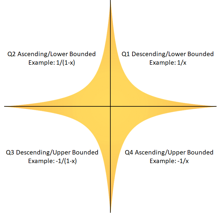
Refer to caption — Figure 6.1. Quadrants of Primitives

Let $I\subseteq J$ be an interval with endpoint coordinates $a,b$ , such that $J$ contains the endpoints $a,b$ . (If $J$ is the circle we allow $a,b$ to represent the same circle point, but require $b=a+1$ ). Recall $\phi_{J\mathbb{\mathbb{R}}}$ is a primitive on $I$ if $\phi$ vanishes outside $I$ , is monotone on $I$ , and has a bound (ie at least one of $\inf\phi$ or $\sup\phi$ exists). Note that a primitive function which is constant is both ascending and descending on $I$ , but any other primitive is either ascending or descending.

A primitive is called upper bounded if $\sup\phi$ exists, and lower bounded if $\inf\phi$ exists. It is called a bounded primitive if both bounds exist, and an unbounded primitive otherwise. We can therefore classify an unbounded primitive by whether it is ascending or descending (A or D) and whether it is upper or lower bounded (U or L).

Let us write the set of Descending, Lower bounded primitives on $I$ as DL, we similarly define the sets AL, AU, and DU. An unbounded primitive belongs to precisely one of these sets, but a bounded primitive is both upper and lower bounded and so will belong to both AU and AL, or to both DU and DL, except for the case of a constant function which belongs to all 4 sets. Note that DL is closed under addition and contains the constant primitive 0. It therefore forms a commutative monoid. Further it forms a module over the semi-ring $\mathbb{R}^{+}=\{x\in\mathbb{R}:x\geq 0\}$ . The same applies to each of the other 3 sets.

Note that if $\phi$ is a primitive on $I$ , then so is $-\phi$ . Further, if $I$ is either open or closed (ie not semi-open) then $\overline{\phi}(x)\coloneqq\phi(a+b-x)$ is also a primitive on $I$ , and hence so is $-\overline{\phi}$ . Finally $\overline{-\phi}(x)=(-\phi)(a+b-x)=-\overline{\phi}(x)$ .

Let $\mathcal{F}$ be a family of primitives of $I$ . Then $-\mathcal{F}\coloneqq\{\phi:-\phi\in\mathcal{F}\}$ is clearly also a family of primitives of $I$ . If $I$ is either open or closed we can also define another family of primitives $\overline{\mathcal{F}}\coloneqq\{\phi:\overline{\phi}(a+b-x)\in\mathcal{F}\}$ , and then $\overline{-\mathcal{F}}=-\overline{\mathcal{F}}=\{\phi:-\overline{\phi}\in\mathcal{F}\}$ is a 4th family. We call the set $\{\mathcal{F},-\mathcal{F}.\overline{\mathcal{F}},-\overline{\mathcal{F}}\}$ the dual quadrants of $\mathcal{F}$ (under the dualities $-,\bar{.}$ ). Note that the set $\{DL,AU,DU,AL\}$ comprises the dual quadrants of each of its 4 members when $I$ is open or closed (but not semi-open), and fixing $DL$ this gives $AU=-DL,AL=\overline{DL},DU=-\overline{DL}$ .

If $\phi$ is a primitive of $I$ which has a lower bound of 0 (ie $\phi\geq 0$ on $I$ ) then we say $\phi$ is a positive primitive on $I$ , and if $\phi\leq 0$ we say $\phi$ is negative. We denote the set of descending positive primitives on $I$ as $\Phi(I)$ , and note this is a sub-monoid of $DL$ ( $\Phi(I)\subset DL(I)$ ). Then the dual quadrant $-\Phi(I)\subset AU(I)$ is the monoid of ascending negative primitives. If $I$ is open or closed, we can also identify the other dual quadrants as the monoids $\overline{\Phi}(I)\subset AL(I),-\overline{\Phi}(I)\subset DU(I)$ .

Positive and negative primitives have the important properties that they can be extended and translated in $J$ .

If $\phi\in\Phi(I)$ and $K$ is a right extension of $I$ (ie $x\in K\backslash I\,\Rightarrow\,x\geq b$ where $b$ is the right endpoint of $I$ ), then $\phi\in\Phi(K)$ so that $\Phi(I)\subset\Phi(K)$ . Similarly $-\Phi(I)\subset-\Phi(K)$ , and if $K^{\prime}$ is a left extension of $I$ (and open or closed with $I$ ) then also $\overline{\Phi}(I)\subset\overline{\Phi}(K^{\prime}),-\overline{\Phi}(I)\subset-\overline{\Phi}(K^{\prime})$ .

We now assume $I=(a,b)$ is open. Let $K=|c,d|$ (where we set $c=0,d=1$ when $K$ is the circle $[0,1)$ ). If $\phi\in\Phi(I)$ we can define the translation $T\phi(x)=\phi(x+(a-c))$ and then $T\phi\in\Phi(c,c+(b-a))$ . By the remarks on extension above we can write $T\phi\in\Phi(c,d)$ and $-T\phi\in-\Phi(c,d)$ . In particular when $K$ is the circle, $T\phi\in\Phi(0,1),-T\phi\in-\Phi(0,1)$ . Similarly if $\phi\in\overline{\Phi}(I)$ we define the translation $\overline{T}\phi(x)=\phi((d-b)+x))$ and then $\overline{T}\phi\in\overline{\Phi}(d-(b-a),d)$ which we can extend to $\overline{T}\phi\in\overline{\Phi}(c,d)$ and $-\overline{T}\phi\in-\overline{\Phi}(c,d)$ . In particular when $J$ is the circle, $\overline{T}\phi\in\overline{\Phi}(0,1),-\overline{T}\phi\in-\overline{\Phi}(0,1)$ . In summary, positive and negative primitives on an open interval $I$ can be translated to primitives on the interior of $K$ .

Note that a monotone function on a closed interval is BV. Since a primitive $\phi$ on $I$ vanishes outside $I$ , if $I$ is closed $\phi$ is BV (and hence LBV) on the whole of $J$ . If $I$ is open then $\phi$ is LBV on $I$ (by 61) and $LBV$ outside the closure of $I$ , and also $LBV$ at the bounded endpoint of $I$ .

6.4. Representation of functions by primitives

Recall we denote the set of points of locally bounded variation $LBV(\phi)$ , and its complement $UBV(\phi)$ . We have shown $LBV(\phi)$ is a union of disjoint open intervals, although it is important to note that this includes the possibilities $LBV(\phi)=\mathbb{T}$ (when $\phi$ is BV on the whole circle) and $LBV=\emptyset$ (for example $\phi(x)=\left\llbracket x=\frac{p}{q},(p,q)=1\right\rrbracket q$ is unbounded everywhere and so is not locally bounded anywhere). Otherwise there is an at most countable set of disjoint open intervals $I_{k}=(x_{k}^{L},x_{k}^{R})$ with $LBV(\phi)=\bigcup_{k}I_{k}$ and $x_{k}^{L},x_{k}^{R}\in UBV(\phi)$ . We will assume $LBV(\phi),UBV(\phi)\neq\emptyset$ going forward. We can now define the observables $\phi_{U}x=\left\llbracket x\in UBV(\phi)\right\rrbracket\phi x$ and $\phi_{i}=\left\llbracket x\in(x_{i}^{L},x_{i}^{R})\right\rrbracket\phi$ , which enables us to write $\phi=\phi_{U}+\sum_{i}\phi_{i}$ with $UBV(\phi_{i})=\{x_{i}^{L},x_{i}^{R}\}$ . In the special case of $\phi$ having a single UBV point $x$ , we get $x_{1}^{L}=x_{1}^{R}=x$ , otherwise the endpoints are all distinct.

Note that for a normalised function, by definition $\phi_{U}=0$ .

We can now extend the Jordan Decomposition theorem from BV functions to LBV functions:

Lemma 68 (Jordan Decomposition of LBV).

If $\phi$ is LBV on an (non-empty) open interval $I=(a,b)$ then for each point $m\in(a,b)$ there is a canonical decomposition into primitives on $I$ , namely $\phi=\phi(m)+\sum_{i=1}^{4}\phi_{i}$ where $\phi_{1}\in\Phi(a,m),\,\phi_{2}\in-\Phi(a,m),\,\phi_{3}\in\overline{\Phi}(m,b),\,\phi_{4}\in-\overline{\Phi}(m,b)$ .

Proof.

We partition $\phi$ into left and right functions $\phi^{L}=\left\llbracket x\in(a,m)\right\rrbracket(\phi(x)-\phi(m)),\,\phi^{R}=\left\llbracket x\in(m,b)\right\rrbracket(\phi(x)-\phi(m))$ .We now define the left and right variations of $\phi$ for $a<x<b$ by $V^{L}(x)=\left\llbracket x\in(a,m)\right\rrbracket\operatorname{Var}_{[x,m]}\phi,\,V^{R}(x)=\left\llbracket x\in(m,b)\right\rrbracket\operatorname{Var}_{[m,x]}\phi$ (the total variation of $\phi$ over $(x,m),(m,x)$ respectively). These functions are well defined since $\phi$ is BV on each interval $(x,m)$ or $(m,x)$ . We now define the difference functions $D^{L}(x)=V^{L}(x)-\phi^{L}(x),\,D^{R}(x)=V^{R}(x)-\phi^{R}(x)$ . Note that these 4 defined functions all vanish outside $(a,m)$ or $(m,b)$ and are monotone and positive and hence positive primitives on their domains. $V^{L},D^{L}$ are both decreasing and so $V^{L},D^{L}\in\Phi(a,m)$ , whereas $V^{R},D^{R}$ are increasing and so $V^{R},D^{R}\in\overline{\Phi}(m,b)$ . But now $\left\llbracket x\in(a,b)\right\rrbracket\phi(x)=\phi(m)+V^{L}(x)-D^{L}(x)+V^{R}(x)-D^{R}(x)$ and the result follows. ∎

We can combine (6.1) and Lemma (68) to obtain:

Theorem 69 (Decomposition Theorem).

Given an observable $\phi_{J\mathbb{R}}$ then $LBV(\phi)$ is an at most countable union of disjoint open intervals $I_{k}=(a_{k},b_{k})$ , and $\phi=\phi_{U}+\sum_{k}\phi_{k}$ where $\phi_{U}=\left\llbracket x\in UBV(\phi)\right\rrbracket\phi$ and $\phi_{k}$ is an LBV function on $I_{k}$ . Further, given $m_{k}\in I_{k}$ we have the representation of $\phi_{k}$ in terms of primitives given by $\phi_{k}=\phi(m_{k})+\sum_{j=1}^{4}\phi_{kj}$ where $\phi_{k1}\in\Phi(a_{k},m_{k}),\,\phi_{k2}\in-\Phi(a_{k},m_{k}),\,\phi_{k3}\in\overline{\Phi}(a_{k},m_{k}),\,\phi_{k4}\in-\overline{\Phi}(a_{k},m_{k})$ .

7. Homogeneous Birkhoff Sums of unbounded observables

7.1. Introduction

In the last section we established that if $\phi_{\mathbb{TR}}$ is an observable on the circle we have the decomposition $\phi=\phi_{U}+\sum_{k\in K}\phi_{k}$ into (at most countable) functions of disjoint support, where each $\phi_{k}$ is LBV with its support in an open interval $I_{k}$ . We also showed we can decompose each $\phi_{k}$ into a sum of 4 primitive functions $\phi_{ki}$ from each quadrant of $\Phi(I)$ . Since $S_{N}$ is linear this means we have reduced the study of $S_{N}(\phi,x)$ to the study of $S_{N}(\phi_{U},x)$ and the study of $S_{N}(\phi_{ki},x)$ with $\phi_{ki}$ primitive. We will generally be concerned with sums for which $x+r\alpha$ never coincides with an unbounded point of $\phi$ so that $S_{N}(\phi_{U},x)=0$ . This means we can replace $\phi$ by its normalised form $\phi^{Norm}$ (which vanishes on the set of unbounded points of $\phi$ ) without changing the overall sum. In this section we concentrate our attention on the study of $S_{N}(\phi,x)$ for primitive $\phi$ .

Now suppose $\phi$ is a primitive on the directed interval $(a,b)$ . If $\phi$ is unbounded at $a$ then $\phi_{a}\coloneqq x_{\mathbb{T}}\rightarrow\phi\{x+a\}$ is a primitive on $(0,1)$ , unbounded at $0^{+}$ . Similarly if $\phi$ is unbounded at $b$ then $\phi_{b}\coloneqq x_{\mathbb{T}}\rightarrow\phi\{x-b\}$ is a primitive on $(0,1)$ , unbounded at $1^{-}$ . Then $S_{N}(\phi,x_{0})=S_{N}(\phi_{a},x_{0}-a)$ and $S_{N}(\phi,x_{0})=S_{N}(\phi_{b},x_{0}+b)$ which means we can reduce the study of Birkhoff sums of general primitives to the study of Birkhoff sums of primitives on $(0,1)$ . We will now assume $\phi$ is a primitive on $(0,1)$ .

Recall that we call $S_{N}(\phi,x)$ a homogeneous sum when $x=0$ and inhomogeneous otherwise.

The general case of an inhomogeneous sum $S_{N}(\phi,x)$ is challenging. This may seem surprising because we can easily convert an inhomogeneous sum to a homogeneous sum by defining $\phi_{c}(x)=\phi(x+c)$ , and then $S_{N}(\phi,x_{0})=S_{N}(\phi_{x_{0}},0)$ . The problem is that in general $\phi_{x_{0}}$ will not then be a primitive on $(0,1)$ , and the underlying problem has not been simplified.

Fortunately homogeneous sums are sufficient to address a high proportion of problems of interest (including the cases described in the abstract of this paper).. Given that this paper is already somewhat lengthy, we therefore content ourselves with postponing consideration of inhomogeneous sums to another paper, and restrict this paper to the homogeneous case.

We will now use the results on the sequential distribution of $(r\alpha)$ from section 5 to develop estimates of the homogeneous sum $S_{N}\phi\coloneqq S_{N}(\phi,0)=\sum_{r=1}^{N}\phi(r\alpha)$ when $\phi$ is a monotonic function on $(0,1)$ . We will use another variant of notation $S_{N}(x)\coloneqq S_{N}(\phi,x)=\sum_{r=1}^{N}\phi(x+r\alpha)$ , noting carefully that this is semantically distinct from the homonymous notation $S_{N}(x)\coloneqq\sum_{r=1}^{N}x_{r}$ of section 4.

The restriction to monotone functions might at first seem restrictive. Classical studies on sums of bounded functions tend to focus on functions of bounded variation as the primary objects of interest. However since any function of bounded variation can be represented as the sum of two monotonic functions (one increasing, one decreasing), a focus on monotone functions is not a limitation, but rather a recognition of the fact that monotonic functions in fact lie slightly deeper.

We will first establish some duality results which reduce the number of cases we will need to consider. We will use the Source-Target Magma theory developed in Section 3, where we put the source $S=(0,1)$ with involution $\sigma_{S}\coloneqq x\mapsto(1-x)$ and target $T=\mathbb{R}$ with involution $\tau_{S}\coloneqq x\mapsto-x$ .

7.2. Dual Relations for Birkhoff Functionals

In this section we will explore the use of dualities to reduce the number of cases we will need to consider when we look at bounds for Birkhoff sums. We will exploit both the quite general Source and Target dualities investigated in Section 3, and also a more specialised quasiperiodic duality which arises in the context of Continued Fraction theory.

These dualities arise under the operation of various involutions, and we will call fixed points of an involution self-conjugate under that involution.

We will also define a duality which combines the effects of the Source and Quasiperiodic involutions. As this will be an important duality for us, we will call it simply the Double Duality, and its fixed points are the double self-conjugate points.

Source-Target Dualities in Birkhoff Sums on the circle Recall that a Birkhoff sum $S_{N}\phi$ can be regarded as a functional operator $\left(S_{N}\right)_{(\mathbb{TR})\mathbb{R}}$ acting on the function $\phi_{\mathbb{TR}}$ . Note that since the orbit $(r\alpha)$ avoids the origin, the sum $S_{N}\phi_{\mathbb{TR}}=\sum_{1}^{N}\phi_{\mathbb{TR}}(r\alpha)$ is identical in value with the sum $S_{N}\phi_{S\mathbb{R}}\left\{r\alpha\right\}$ where $\phi_{\mathbb{TR}}$ has been replaced by its restriction to the interval $S=(0,1)$ , and the Birkhoff Sum functional $\left(S_{N}\right)_{(\mathbb{TR})\mathbb{R}}$ becomes $\left(S_{N}\right)_{(S\mathbb{R})\mathbb{R}}$ .

Using this observation, we can now apply the theory developed in Section 3. In particular we will build on the example application given in Subsection 3.4. We take as the real intervals $S\coloneqq(0,1)$ and $T\coloneqq\mathbb{R}$ (again equipped with the endorelations $R_{S}=R_{T}=\leq_{\mathbb{R}}$ ). We now set the source involution $\sigma_{S}$ to be the circle involution $\overline{.}:x\mapsto\{1-x\}$ but restricted to $(0,1)$ (where we note it is still an involution and can be written $x\mapsto 1-x$ ), and we set the target involution to be $\tau_{T}\coloneqq x_{\mathbb{R}}\mapsto-x$ .

Note that now the source pull up of $\sigma_{S}$ is $\sigma_{ST}=(\overline{.})_{ST}\coloneqq\phi_{ST}\mapsto\phi\circ\text{$\sigma_{S}$}$ , ie $\overline{\phi}\alpha\coloneqq\phi\overline{\alpha}$ . Similarly the target pull up of $\tau_{T}$ is $\tau_{ST}=-_{ST}\coloneqq\phi\mapsto-_{T}\circ\phi$ , ie $\left(-_{ST}\phi\right)\alpha\coloneqq-_{\mathbb{R}}\left(\phi\alpha\right)$ . Again we can pull up to Level 2, to get $\sigma_{(ST)T}\coloneqq A_{(ST)T}\mapsto A\circ\sigma_{ST}$ , ie $\overline{A}\phi\coloneqq A\overline{\phi}$ and similarly $\left(-_{(ST)T}A\right)\phi\coloneqq-_{\mathbb{R}}\left(A\phi\right)$ .

If we further assume that $A$ is a $\tau-$ morphism this means $A(-_{ST}\phi)=-_{\mathbb{R}}\left(A\phi\right)$ .

In this source-target environment we also have further structure than in 3.4 since $T=\left(\mathbb{R},+_{\mathbb{R}},\times_{\mathbb{R}}\right)$ is a field. The pull up the binary operations of $T$ to $ST$ induces an algebra of functions over $T$ (where $\lambda_{T}\phi_{ST}\,+_{ST}\,\mu_{T}\psi_{ST}$ and $\phi\,\times_{ST}\,\psi$ have their natural meanings). It is easily verified that the involutions $\sigma_{ST},\tau_{ST}$ are are then linear in both $+_{ST},\times_{ST}$ . The same argument applies analogously to the algebra $(ST)T$ of functionals over $T$ .

If $\Psi\subset ST$ is self-conjugate under $\sigma\tau$ , the Example application of Subsection 3.4 now applies, giving us:

(7.1)

\displaystyle A_{1}\leq_{\Psi}A_{2}

\displaystyle\Leftrightarrow\sigma A_{1}\leq_{\overline{\Psi}}\sigma A_{2}\Leftrightarrow\sigma^{/}A_{1}\leq_{\overline{\Psi}}\sigma^{/}A_{2}\Leftrightarrow\sigma\sigma^{/}A_{1}\leq_{\Psi}\sigma\sigma^{/}A_{2}

\Leftrightarrow\tau A_{1}\leq_{\Psi}^{Op}\tau A_{2}\Leftrightarrow\sigma\tau A_{1}\leq_{\overline{\Psi}}^{Op}\sigma\tau A_{2}\Leftrightarrow\sigma^{/}\tau A_{1}\leq_{\overline{\Psi}}^{Op}\sigma^{/}\tau A_{2}\Leftrightarrow\sigma\sigma^{/}\tau A_{1}\leq_{\Psi}^{Op}\sigma\sigma^{/}\tau A_{2}

We can go further in the case that $A_{1},A_{2}$ are $\tau-$ morphisms. We use the results of (3.10) to obtain from $A_{1}\leq_{\Psi}A_{2}$ :

(7.2)

\displaystyle A_{1}\leq_{\Psi}A_{2}\Leftrightarrow\sigma A_{1}\leq_{\overline{\Psi}}\sigma A_{2}\Leftrightarrow\tau A_{1}\leq_{\overline{\Psi}}\tau A_{2}\Leftrightarrow\sigma\tau A_{1}\leq_{\Psi}\sigma\tau A_{2}

\Leftrightarrow\tau A_{1}\leq_{\Psi}^{Op}\tau A_{2}\Leftrightarrow\sigma\tau A_{1}\leq_{\overline{\Psi}}^{Op}\sigma\tau A_{2}\Leftrightarrow A_{1}\leq_{\overline{\Psi}}^{Op}A_{2}\Leftrightarrow\sigma A_{1}\leq_{\Psi}^{Op}\sigma A_{2}

We pick out the first and last dual relations as being of particular use to us later in this Section:

(7.3)

A_{1}\leq_{\Psi}A_{2}\Leftrightarrow\sigma A_{2}\leq_{\Psi}\sigma A_{1}

Remark 70.

Let $\Theta\subset ST$ be a set of functions which are descending (ascending) on $S$ . Now $\sigma_{ST}\tau_{ST}\Theta=-\overline{\Theta}$ and this is also a set of descending (ascending) functions. Recall $\Psi(\Theta)\coloneqq\Theta\bigcup\sigma\tau\Theta=\Theta\bigcup-\overline{\Theta}$ is self-conjugate under $\sigma\tau$ , as is also $\sigma\Psi=\overline{\Psi}=\overline{\Theta}\bigcup-\Theta$ . So in these cases of $\Phi$ , $\Psi$ is a self-conjugate set of descending (ascending) functions, and $\overline{\Psi}$ is a self-conjugate set of ascending (descending) functions for which the dual relations in (7.1) apply, and further (7.2) apply when $A_{1},A_{2}$ are $\tau-$ morphisms. There are important two special cases:

(1)

When $\Theta=\Psi$ is the set of all monotonic descending (or monotonic ascending, or simply all monotonic) functions
(2)

When $\Psi=\Phi\bigcup\sigma\tau\Phi$ where $\Phi$ is the monoid of positive descending primitives from (**).

Quasi-Period Duality

In this section we explore a specialised duality which arises in the context of continued fraction developments. We will use some of the Source/Target Duality theory from the previous section, but now in our specific environment of Birkhoff sums over rotations. Indexed Families Recall that it is sometimes convenient to call a function $\iota_{IX}:I\rightarrow X$ an index function. We then call $I$ the index set, and $x_{i}\coloneqq\iota(i)$ an indexed element. We call the collection $(x_{i})_{i\in I}$ an indexed family (indexed by $I$ ). If $I=\{i\}_{i=1}^{n}$ we also write the indexed family as $(x_{i})_{i=1}^{n}$ .

Remark 71.

It is particularly important to note that $(x_{i})$ is not a set if $\iota$ is not injective (it is a collection containing identical elements). This means we must be particularly careful if we wish to define functions on the set $X=\{x_{i}\}$ making use of the index $i$ . For example, given an endomorphism $f_{II}$ of $I$ we can define the pull back function $g_{IX}=\iota\circ f$ which is a well-defined index function from $I$ to $X$ . It is then tempting to think that we can then also define a derived endomorphism $h_{XX}:x_{i}\mapsto x_{f(i)}$ but this is not the case in general: if $h$ exists and $\iota(i)=\iota(j)$ then $x_{f(i)}=h(x_{i})=h(x_{j})=x_{f(j)}$ and this is not the case for general $f$ , even if $f$ is a bijection. In general then, $h_{XX}$ is a relation (or multi-valued function).

Quasi-Period Indexed Families Recall (10) that we denote the sequence of quasiperiods of $\alpha_{\mathbb{R}\backslash\mathbb{Q}}$ as $(q_{r}^{\alpha}){}_{r=0}^{\infty}$ , and that for $\alpha\in(0,\frac{1}{2})\backslash\mathbb{Q}$ we have $q_{r}^{\alpha}=q_{\overline{r}}^{\overline{\alpha}}$ where $\overline{\alpha}=\{1-\alpha\}$ and $\overline{r}=r+1$ . This result reveals a non-trivial duality which we will develop in this section.

Note first that we have here two maps with the homonymous notation ${}^{\prime}\overline{.}^{\prime}$ . We can extend both to involutions as follows. The first is defined on $\mathbb{I}=[0,1)$ by $\left(\overline{.}\right)_{\mathbb{I}}\coloneqq\alpha\mapsto\{1-\alpha\}$ (note that $\overline{0}=0$ is fixed point). The second needs slightly more care in definition: recalling $\mathbb{N}=\mathbb{N}^{+}\bigcup\{0\}$ we take the disjoint union $\mathbb{N}_{2}=\mathbb{N}\bigsqcup\mathbb{N}^{+}$ and define the involution $\left(\overline{.}\right)_{\mathbb{N}_{2}}$ by: $\overline{r_{\mathbb{N}}}\coloneqq(r+1)_{\mathbb{N}^{+}}$ and $\overline{r_{\mathbb{N}^{+}}}\coloneqq(r-1)_{\mathbb{N}}$ . We can now use these two involutions to define a product involution $\left(\overline{.}\right)_{\mathbb{I}}\times\left(\overline{.}\right)_{\mathbb{N}_{2}}$ on a suitable set as follows:

Definition 72.

The QuasiPeriod index set $QPI=\left(QPI_{Set},\overline{.}\right)$ has as its underlying set the strict subset $QPI_{Set}\subset\mathbb{I}\times\mathbb{N}$ defined by

QPI\coloneqq\left\{(\alpha,r):\alpha\in\mathbb{I}\backslash\mathbb{Q}\>\&\>r\geq\left\llbracket\alpha\geq\frac{1}{2}\right\rrbracket\right\}

It is equipped with the Quasiperiod involution $Q_{QPI}$ defined by $Q(\alpha,r)\coloneqq\overline{(\alpha,r)}=(\overline{\alpha},\overline{r})$ where $\overline{\alpha}\coloneqq\{1-\alpha\}$ and $\overline{r}\coloneqq r+(-1)^{\left\llbracket\alpha>\frac{1}{2}\right\rrbracket}$ .

A QP indexed family (QPI family) $X=\left\{(x_{r}^{\alpha}),\iota_{(QPI)X}\right\}$ is a family $X=(x_{r}^{\alpha})$ indexed by the QP index set $QPI$ using the index map $\iota_{(QPI)X}:(\alpha,r)_{QPI}\mapsto x_{r}^{\alpha}$ ). There is usually no need to specify the index map, in which case we simply write $X=(x_{r}^{\alpha})$ . Points satisfying $x_{\overline{r}}^{\overline{\alpha}}=x_{r}^{\alpha}$ we call QP self-conjugate. . If the index map is independent of $\alpha$ , ie for each $r$ , $\iota(\alpha,r)=x_{r}$ for every $\alpha$ , we will also allow ourselves to write the family as $(x_{r}^{\alpha})=(x_{r})$ . Similarly if $\iota$ is independent of $r$ , we will write the family as $(x^{\alpha})$ , and as $(x)$ if $\iota$ is a constant map.

Remark 73.

Note that $(\alpha,r)\in QPI$ means $r\geq 0$ for $\alpha<\frac{1}{2}$ and $r\geq 1$ for $\alpha>\frac{1}{2}$ . In particular this means that a QPI family $(x_{r}^{\alpha})$ contains no element $x_{0}^{\alpha}$ for $\alpha>\frac{1}{2}$ .

Note that a QP indexed family may be further indexed by other index sets, eg the family $(x_{rz}^{\alpha})$ is indexed by $QPI\times Z$ , but the QP involution only affects the QP index within the family, ie $x_{rz}^{\alpha}=\iota\left((\alpha,r),z\right)$ and $\iota\left((\overline{\alpha},\overline{r}),z\right)=x_{\overline{r}z}^{\overline{\alpha}}$ .

In line with Remark 71 we cannot assume that there is an induced qp involution $Q_{X}\coloneqq x_{r}^{\alpha}\mapsto x_{\overline{r}}^{\overline{\alpha}}$ on a QPI family $X=(x_{r}^{\alpha})$ if the index map is not injective. However in many (but not all ) important cases, the function $x_{r}^{\alpha}\mapsto x_{\overline{r}}^{\overline{\alpha}}$ is well-defined (and then the induced function is also an involution since $Q_{QPI}$ is itself an involution). When this is the case some individual proofs below could be simplified. However our overall presentation is simplified by having a single set of proofs which work whether an induced involution is defined or not. Hence we will NOT generally assume $Q\coloneqq x_{r}^{\alpha}\mapsto x_{\overline{r}}^{\overline{\alpha}}$ is well-defined in the sequel.

We now define a duality which will prove important in later sections. This is a hybrid using both the QP involution and the source involution $\left(\overline{.}\right)_{\mathbb{II}}\coloneqq\alpha\mapsto{1-\alpha}$ .

Definition 74 (Double Dual).

Given a QPI family of functions $(\phi_{r}^{\alpha})$ , we call the derived family $\left(\overline{\phi_{\overline{r}}^{\overline{\alpha}}}\right)$ the family of the double dual functions of $(\phi_{r}^{\alpha})$ . For convenience we will use the simplified notation $\overline{\phi}_{r}^{\alpha}\coloneqq\overline{\phi_{\overline{r}}^{\overline{\alpha}}}$ . When $\overline{\phi}_{r}^{\alpha}=\phi_{r}^{\alpha}$ we say $\phi_{r}^{\alpha}$ is double self-conjugate.

Remark 75.

It is important note that following Remark (**) we cannot regard the Double Dual as a function map because $\overline{\phi}_{r}^{\alpha}\mapsto\phi_{r}^{\alpha}$ may be multi-valued.

Example 76.

Important examples of QPI families

(1)

The quasiperiod index set $QPI$ is itself a QP indexed family using the index map $Id_{QPI}$ . Since $Id$ is injective, in this case the involution $Q:(\alpha,r)\mapsto\overline{(\alpha,r)}$ exists trivially.
(2)

A scalar qp family $\left(\lambda_{r}^{\alpha}\right)$ with each $\lambda_{r}^{\alpha}\in\mathbb{R}$ . Important examples are $q_{r}^{\alpha},a_{r+1}^{\alpha},b_{r}^{\alpha}$ (where these symbols have their standard meanings). Note that these particular examples are also qp self-conjugate (eg $q_{r}^{\alpha}=q_{\overline{r}}^{\overline{\alpha}}$ ) with the single exception of $a_{r+1}^{\alpha}$ for $\alpha<\frac{1}{2},r=0$ when $a_{2}^{\overline{\alpha}}=a_{1}^{\alpha}-1$ . Scalar families will not generally have injective index maps ( $Q_{{}_{\left(\lambda_{r}^{\alpha}\right)}}$ is not well defined), although the identity function serves as a partial qp involution when restricted to the set of self-conjugate elements.
(3)

The particular scalar qp family $\left(E_{r}^{\alpha}\right)$ where $E_{r}^{\alpha}\coloneqq E_{r}=\left\llbracket r\,\mathrm{even}\right\rrbracket$ (so the family $\left(E_{r}^{\alpha}\right)$ is independent of $\alpha$ ). Note $E_{\overline{r}}^{\overline{\alpha}}=O_{r}^{\alpha}$ and $O_{\overline{r}}^{\overline{\alpha}}=E_{r}^{\alpha}$ and so $\left(E_{r}^{\alpha}\right)=\left(O_{r}^{\alpha}\right)$ .The index map $\iota:(\alpha,r)\mapsto E_{r}^{\alpha}=E_{r}$ is clearly not injective, but in fact the induced involution $Q_{\left(E_{r}^{\alpha}\right)}$ does exist.
(4)

Given a scalar qp family $\{\lambda_{r}^{\alpha}\}$ we can form new scalar families such as $\left\{f_{\mathbb{\mathbb{R}R}}(\lambda_{r}^{\alpha})\right\}$ or $\left\{\phi_{\mathbb{IR}}(\lambda_{r}^{\alpha})\right\}$ (when $\lambda_{r}^{\alpha}\in\mathbb{I}$ ), and $\left\llbracket P(\lambda_{r}^{\alpha})\right\rrbracket$ (where $P$ is a proposition). If $\lambda_{r}^{\alpha}$ is qp self conjugate, so are $f(\lambda_{r}^{\alpha})$ , $\phi(\lambda_{r}^{\alpha})$ and $\left\llbracket P(\lambda_{r}^{\alpha})\right\rrbracket$ . In particular $\phi\left(\frac{1}{q_{r}^{\alpha}}\right)$ is qp self conjugate for $r>0$ .
(5)

The qp family of qp index functions $n^{\alpha}:\mathbb{N}^{+}\rightarrow\mathbb{N}$ defined by $n^{\alpha}(N)\coloneqq\max\{t:q_{t}^{\alpha}\leq N\}$ . Note we have dropped $r$ from the notation to indicate that these functions are independent of $r$ , ie for any $r$ , $n_{r}^{\alpha}=n^{\alpha}$ . Note also that we can now write the Ostrowski representation of $N$ as $N=\sum_{r=\left\llbracket\alpha>\frac{1}{2}\right\rrbracket}^{n^{\alpha}(N)}b_{r}q_{r}$ , and also that we can now write the relationship between the indexes $n^{\alpha},n^{\overline{\alpha}}$ as $n^{\overline{\alpha}}(N)=n^{\alpha}(N)+(-1)^{\left\llbracket\alpha>\frac{1}{2}\right\rrbracket}$ . In particular this gives $q_{n^{\alpha}}^{\alpha}=q_{n^{\overline{\alpha}}}^{\overline{\alpha}}.$
(6)
The qp scalar family $c_{rst}^{\alpha}$ for some symbol $c$ :
1. (a)
  
  When $c$ is the null symbol we will simply write $\alpha_{rst}$ . The QP conjugate is $\overline{\alpha}_{\overline{r}st}$ , and since $\overline{\alpha}_{\overline{r}st}=\{1-\alpha_{rst}\}=\overline{\alpha_{rst}}$ qp involution and source involution coincide on $\mathbb{I}\backslash\mathbb{Q}$
2. (b)
  
  When $c$ is an observable symbol, eg $\phi$ , we write $\phi_{rst}^{\alpha}\coloneqq\phi(\alpha_{rst})$ with QP conjugate $\phi_{\overline{r}st}^{\overline{\alpha}}=\phi(\overline{\alpha}_{\overline{r}st})=\phi(\overline{\alpha_{rst}})=\overline{\phi}_{rst}^{\alpha}$ , and again qp involution and source involution coincide

. QPI Families of Operators

Let $\mathscr{X}$ be the set of QPI families of functionals (families whose elements lie in $(ST)T$ ), and let $\left(X_{r}^{\alpha}\right),\left(Y_{r}^{\alpha}\right)$ 2 members of $\mathscr{X}$ . Define $Z_{r}^{\alpha}\coloneqq\lambda X_{r}^{\alpha}+\mu Y_{r}^{\alpha}$ . By this definition $Z_{\overline{r}}^{\overline{\alpha}}\coloneqq\lambda X_{\overline{r}}^{\overline{\alpha}}+\mu Y_{\overline{r}}^{\overline{\alpha}}$ and hence $\left(Z_{r}^{\alpha}\right)$ is also a QPI family, and we can write $\left(Z_{r}^{\alpha}\right)=\lambda_{T}\left(X_{r}^{\alpha}\right)\,+_{\mathscr{X}}\,\mu_{T}\left(Y_{r}^{\alpha}\right)$ to mean for each $(\alpha,r)$ that $Z_{r}^{\alpha}=\lambda X_{r}^{\alpha}+\mu Y_{r}^{\alpha}$ . Note then $\mathscr{X}$ is a vector space over $T$ , and $+_{\mathscr{X}}$ is the pull up of $+_{T}$ to $\mathscr{X}$ . Similarly we can also pull up $\times_{T}$ to $\mathscr{X}$ so that $\left(X_{r}^{\alpha}\right)\times\left(Y_{r}^{\alpha}\right)$ is again a QPI family, and so $\mathscr{X}$ is also an algebra over $T$ .

Recall also that that when $ST$ is equipped with an involution $\upsilon{}_{ST}$ then this induces a pullup involution $\upsilon_{(ST)T}$ defined by $\upsilon_{(ST)T}(X)\coloneqq X\circ\upsilon_{ST}$ which is also linear in $+_{ST},\times_{ST}$ . Again given a QPI family $\left(X_{r}^{\alpha}\right)$ we can define the pullup involution $\upsilon_{\mathscr{X}}$ by $\upsilon_{\mathscr{X}}\left(\,\left(X_{r}^{\alpha}\right)\,\right)=\left(\upsilon_{(ST)T}X_{r}^{\alpha}\right)$ and again this is linear in $+_{\mathscr{X}},\times_{\mathscr{X}}$ , so that $\upsilon_{\mathscr{X}}$ is an algebra automorphism.

In particular we have proved:

Proposition 77 (Linearity of Double Dual).

If $Z_{r}^{\alpha}=\sum_{i=1}^{k}X_{ir}^{\alpha}\times Y_{ir}^{\alpha}$ then $\left(Z_{r}^{\alpha}\right)$ is a QPI family and $\overline{Z_{\overline{r}}^{\overline{\alpha}}}=\sum_{i=1}^{k}\overline{X_{\overline{r}}^{\overline{\alpha}}}\times\overline{Y_{\overline{r}}^{\overline{\alpha}}}$ , ie the double dual of an algebraic combination of $QPI$ families is the same algebraic combination of the double duals

Proof.

We showed above that $\left(Z_{r}^{\alpha}\right)$ is a QPI family. The double dual of $Z_{r}^{\alpha}$ is $\sigma_{(ST)T}Z_{\overline{r}}^{\overline{\alpha}}$ which by definition of $Z_{r}^{\alpha}$ is $\sigma_{(ST)T}\left(\sum_{i=1}^{k}X_{\overline{r}}^{\overline{\alpha}}\times Y_{\overline{r}}^{\overline{\alpha}}\right)$ and the result follows since $\sigma$ is an algebra homomorphism. ∎

Example 78.

Important examples of qp operator families

(1)

Given an operator $X$ we can define the constant qp family $\mathscr{X}_{X}$ in which $X_{r}^{\alpha}\phi=X\phi$ for all $(\alpha,r)\in QPI$ . This family is automatically qp self conjugate ( $X_{\overline{r}}^{\overline{\alpha}}\phi=X\phi=X_{r}^{\alpha}\phi$ ).
(2)

The partition sum operator family $P_{q_{r}^{\alpha}}$ (see Subsection 7.3 for details) is a linear operator family which is Source self conjugate ( $P_{q_{r}^{\alpha}}=\overline{P_{q_{r}^{\alpha}}}$ ), QP self conjugate $(P_{q_{r}^{\alpha}}=P_{q_{\overline{r}}^{\overline{\alpha}}})$ , and hence also double self conjugate ( $P_{q_{r}^{\alpha}}=\overline{P}_{q_{r}^{\alpha}}\coloneqq\overline{P_{q_{\overline{r}}^{\overline{\alpha}}}}$ )
(3)

$\phi\mapsto\phi_{rst}^{\alpha}\coloneqq\phi\left(\alpha_{rst}\right)$ is an (anonymous) linear operator family which is neither source nor qp self conjugate, but is double self conjugate $($ $\phi_{rst}^{\alpha}=\overline{\phi}_{rst}^{\alpha}\coloneqq\overline{\phi_{\overline{r}st}^{\overline{\alpha}}}$ ).
(4)

The family $S_{rs}^{\alpha}\phi=S_{q_{r}}^{\alpha}(\phi,\alpha_{rs})\coloneqq\sum_{t=1}^{q_{r}}\phi_{rst}^{\alpha}$ is double self conjugate since $\phi\mapsto\phi_{rst}^{\alpha}$ is double self conjugate, and hence also the sum $\sum_{s=0}^{b_{r}-1}S_{rs}^{\alpha}$ is double self-conjugate.
(5)

$\phi\mapsto\phi(f(q_{r}^{\alpha}))$ is an (anonymous) linear operator family which is not source self conjugate, but which is qp self conjugate since the qp family $\left(q_{r}^{\alpha}\right)$ is qp self conjugate ( $q_{r}^{\alpha}=q_{\overline{r}}^{\overline{\alpha}}$ ). In particular $\phi\mapsto\phi(\frac{1}{q_{r}^{\alpha}})$ is qp self conjugate.

Recall that in this section we are considering the Source-Target Magma where $S=(0,1),T=\mathbb{R}$ .

Definition 79.

Given two QPI operator families $\left(X_{r}^{\alpha}\right),\left(Y_{r}^{\alpha}\right)$ we will say $\left(X_{r}^{\alpha}\right)$ is dominated by $\left(Y_{r}^{\alpha}\right)$ on $\Theta\subseteq ST$ if for every ( $\alpha,r)\in QPI$ we have $X_{r}^{\alpha}\leq_{\Theta}Y_{r}^{\alpha}$ . We write this as $\left(X_{r}^{\alpha}\right)\leq_{\Theta}\left(Y_{r}^{\alpha}\right)$

Lemma 80 (Domination Duals).

Let $\Psi\subset ST$ be self-conjugate under the involution $\sigma_{ST}\tau_{ST}$ . Given two linear QPI families $\left(X_{r}^{\alpha}\right),\left(Y_{r}^{\alpha}\right)$ of functionals from $(ST)T$ , then we have the following dual results:

\left(X_{r}^{\alpha}\right)\leq_{\Psi}\left(Y_{r}^{\alpha}\right)\Leftrightarrow\left(X_{\overline{r}}^{\overline{\alpha}}\right)\leq_{\Psi}\left(Y_{\overline{r}}^{\overline{\alpha}}\right)\Leftrightarrow\left(\overline{Y_{r}^{\alpha}}\right)\leq_{\Psi}\left(\overline{X_{r}^{\alpha}}\right)\Leftrightarrow\left(\overline{Y_{\overline{r}}^{\overline{\alpha}}}\right)\leq_{\Psi}\left(\overline{X_{\overline{r}}^{\overline{\alpha}}}\right)

Proof.

( $1\Leftrightarrow 2$ ): By definition $\left(X_{r}^{\alpha}\right)=\left(X_{\overline{r}}^{\overline{\alpha}}\right)$ , and so trivially $\left(X_{r}^{\alpha}\right)\leq_{\Psi}\left(Y_{r}^{\alpha}\right)\Leftrightarrow\left(X_{\overline{r}}^{\overline{\alpha}}\right)\leq_{\Theta}\left(Y_{\overline{r}}^{\overline{\alpha}}\right)$ .

( $1\Leftrightarrow 3$ ): Since $\Psi$ is self-conjugate, and $X_{r}^{\alpha},Y_{r}^{\alpha}$ are linear (and hence $\tau-$ morphisms), then by 7.3 we have $X_{r}^{\alpha}\leq_{\Psi}Y_{r}^{\alpha}\Leftrightarrow\overline{Y_{r}^{\alpha}}\leq_{\Psi}\overline{X_{r}^{\alpha}}$ , and the result follows.

( $2\Leftrightarrow 4$ ): This follows by taking the duality ( $1\Leftrightarrow 3$ ) and applying the duality ( $1\Leftrightarrow 2$ ). ∎

Analogous results follow for $\overline{\Psi}$ .

Recall that $S_{rs}^{\alpha}\phi\coloneqq\sum_{t=1}^{q_{r}}\phi_{rst}^{\alpha}$

Corollary 81.

If $\Psi$ is self-conjugate and $\left(X_{r}^{\alpha}\right)$ is linear, $\left(\sum_{s=0}^{b_{r}^{\alpha}-1}S_{rs}^{\alpha}\right)\leq_{\Psi}\left(X_{r}^{\alpha}\right)$ on $\Psi$ if and only if $\left(\overline{X_{\overline{r}}^{\overline{\alpha}}}\right)\leq_{\Psi}\left(\sum_{s=0}^{b_{r}^{\alpha}-1}S_{rs}^{\alpha}\right)$

Proof.

This follows directly from the lemma putting $Y_{r}^{\alpha}=\sum_{s=0}^{b_{r}-1}S_{rs}^{\alpha}$ and using the fact that $b_{r}^{\alpha}$ and $S_{rs}^{\alpha}$ are double self conjugate, and hence by linearity of the double dual (Proposition 77) so is the sum $Y_{r}^{\alpha}$ . ∎

7.3. Partition Sums

We now introduce a set of linear functionals on observables which will form an important part of our Birkhoff Sum estimates.

Definition 82.

Partition Sums. Consider the partition of $[0,1)$ into $k\geq 1$ equal sub-intervals starting from $0$ . We call the $k-1$ points with coordinates $\left\{\frac{t}{k}\right\}_{t=1}^{k-1}$ (ie not including $0$ ) the interior points, and define the partition sum of $\phi$ on the partition to be the sum of values of $\phi$ over the interior points, namely $P_{k}(\phi)=\sum_{t=1}^{k-1}\phi(\frac{t}{k})$ .

Remark 83.

Note that $P_{k}$ is a linear functional of $\phi$ , and that $P_{1}(\phi)$ is an empty sum taking the value $0$ , and that $P_{2}(\phi)=\phi(\frac{1}{2})$ .

Recall from the previous section that we are using the notation $\left(\overline{.}\right)_{\mathbb{T}^{\circ}}$ for the Source involution of the circle $x\mapsto\overline{x}=\{1-x\}$ . This has the pull ups $\left(\overline{.}\right)_{\left(\mathbb{TR}\right)^{\circ}}:\phi\mapsto\overline{\phi}$ , $\left(\overline{.}\right)_{\left((\mathbb{TR})T\right)^{\circ}}:A\mapsto\overline{A}$ defined by $\overline{\phi}x=\phi\overline{x},\overline{A}\phi=A\overline{\phi}$

Proposition 84.

$P_{k}$ is self-conjugate under the Source involution $\left(\overline{\text{.}}\right)_{\mathbb{T}}$ , and if $\phi_{\mathbb{TR}}$ is anti-symmetric then $P_{k}(\phi)=0$

Proof.

By definition, putting $u=k-t$ :

\overline{P_{k}}(\phi)=P_{k}(\overline{\phi})=\sum_{t=1}^{k-1}\phi(1-\frac{t}{k})=\sum_{u=1}^{k-1}\phi(\frac{u}{k})=P_{k}(\phi)

Now if $\phi$ is anti-symmetric on the circle we have $\phi=-\overline{\phi}$ . Since $P_{k}$ is linear $P_{k}\left(\phi\right)=P_{k}\left(-\overline{\phi}\right)=-P_{k}\left(\overline{\phi}\right)=-P_{k}\left(\phi\right)$ , hence $P_{k}(\phi)=0$ . ∎

We will usually be concerned with partition sums $P_{q_{r}^{\alpha}}$ where $q_{r}^{\alpha}$ is a quasiperiod of $\alpha_{\mathbb{T}}$ .

Proposition 85.

$P_{q_{r}^{\alpha}}$ is self-conjugate under the quasiperiod involution $(\alpha,r)\mapsto(\overline{\alpha},\overline{r})$

Proof.

Recall that $q_{r}^{\alpha}$ is itself self-conjugate, ie $q_{r}^{\alpha}=q_{\overline{r}}^{\overline{\alpha}}$ , and the result follows trivially. ∎

7.4. Birkhoff sums of monotonic functions on $(0,1)$

Recall $S_{N}^{\alpha}\phi=\sum_{r=0}^{n^{\alpha}}\sum_{s=0}^{b_{r}-1}S_{rs}^{\alpha}\phi$ where $S_{rs}^{\alpha}\phi=S_{q_{r}^{\alpha}}(\phi,\alpha_{rs})=\sum_{t=1}^{q_{r}^{\alpha}}\phi(\alpha_{rs}+t\alpha)=\sum_{t=1}^{q_{r}^{\alpha}}\phi_{rst}^{\alpha}$ . We will fix $\alpha$ for the moment and drop it from the annotation.

When $q_{r}=1$ we may have $q_{1}=q_{0}=1$ . However in this case we also have $\alpha>\frac{1}{2}$ . Also from (18) $b_{0}=0$ so that the $S_{q_{0}}$ term is not of interest and we can write $S_{N}^{\alpha}\phi=\sum_{r=\left\llbracket\alpha>\frac{1}{2}\right\rrbracket}^{n}\sum_{s=0}^{b_{r}-1}S_{rs}^{\alpha}\phi$

Now for $q_{r}=1$ , $t\in(1..q_{r})$ gives $t\in(1)$ and so $S_{q_{r}}(\alpha_{rs})=\sum_{t=1}^{q_{r}}\phi_{rst}=\phi_{rsq_{r}}$ and similarly for $q_{r}=2$ we have $S_{q_{r}}(\alpha_{rs})=\sum_{t=1}^{q_{r}}\phi_{rst}=\phi_{rsq_{r}}+\phi_{rsq_{r-1}}$ (since $q_{r-1}=1$ ). Combining these results we have for $q_{r}\leq 2$ (and where $b_{r}=0$ gives the empty sum $0$ ):

(7.4)

\sum_{s=0}^{b_{r}-1}S_{rs}^{\alpha}\phi=\sum_{s=0}^{b_{r}-1}\left(\phi_{rsq_{r}^{\alpha}}^{\alpha}+\left\llbracket q_{r}^{\alpha}>1\right\rrbracket\phi_{rsq_{r-1}^{\alpha}}^{\alpha}\right)

Definition 86 (Bounds Operators).

Given $\alpha,N$ , the Bounds Functionals $\left(B_{r}^{\alpha}\right)$ form a QP family of operators in $\left(\mathbb{TR}\right)\mathbb{R}$ defined on observables $\phi$ by:

(7.5)

B_{r}^{\alpha}\phi=\left\llbracket b_{r}^{\alpha}>0\right\rrbracket\left(\left\llbracket q_{r}^{\alpha}>1\right\rrbracket b_{r}^{\alpha}\left(P_{q_{r}^{\alpha}}(\phi)-\overline{\phi}(\frac{1}{q_{r}^{\alpha}})\right)+\left\llbracket 2<q_{r}^{\alpha}<q_{n^{\alpha}}^{\alpha}\right\rrbracket E_{r}^{\alpha}\left(\phi_{r0,q_{r}-q_{r-1}}^{\alpha}-\overline{\phi}\left(\frac{2}{q_{r}^{\alpha}}\right)\right)+\sum_{s=0}^{b_{r}^{\alpha}-1}\left(\phi_{rsq_{r}}^{\alpha}+\left\llbracket q_{r}^{\alpha}>1\right\rrbracket\phi_{rsq_{r-1}}^{\alpha}\right)\right)

Remark 87.

Note this reduces to (7.4) for $q_{r}^{\alpha}\leq 2$ .

Further note that each Bounds Functional is an algebraic combinations of other linear QPI functionals and hence linear .

Lemma 88.

The Bounds Functionals $\left(B_{r}^{\alpha}\right)$ have QP duals $\left(B_{\overline{r}}^{\overline{\alpha}}\right)$ and Double Duals $\left(\overline{B_{\overline{r}}^{\overline{\alpha}}}\right)$ which can be written (when $\alpha$ is fixed):

(7.6)

B_{\overline{r}}^{\overline{\alpha}}\phi=\left\llbracket b_{r}>0\right\rrbracket\left(\left\llbracket q_{r}>1\right\rrbracket b_{r}\left(P_{q_{r}}(\phi)-\overline{\phi}(\frac{1}{q_{r}})\right)+\left\llbracket 2<q_{r}<q_{n}\right\rrbracket O_{r}\left(\overline{\phi}_{r0,q_{r}-q_{r-1}}-\overline{\phi}\left(\frac{2}{q_{r}}\right)\right)+\sum_{s=0}^{b_{r}-1}\left(\overline{\phi}_{rsq_{r}}+\left\llbracket q_{r}>1\right\rrbracket\overline{\phi}_{rsq_{r-1}}\right)\right)

(7.7)

\overline{B_{\overline{r}}^{\overline{\alpha}}}\phi=\left\llbracket b_{r}>0\right\rrbracket\left(\left\llbracket q_{r}>1\right\rrbracket b_{r}\left(P_{q_{r}}(\phi)-\phi(\frac{1}{q_{r}})\right)+\left\llbracket 2<q_{r}<q_{n}\right\rrbracket O_{r}\left(\phi_{r0,q_{r}-q_{r-1}}-\phi\left(\frac{2}{q_{r}}\right)\right)+\sum_{s=0}^{b_{r}-1}\left(\phi_{rsq_{r}}+\left\llbracket q_{r}>1\right\rrbracket\phi_{rsq_{r-1}}\right)\right)

Proof.

Applying the QP involution to the definition (7.5) gives us the QP dual:

B_{\overline{r}}^{\overline{\alpha}}\phi=\left\llbracket b_{\overline{r}}^{\overline{\alpha}}>0\right\rrbracket\left(\left\llbracket q_{\overline{r}}^{\overline{\alpha}}>1\right\rrbracket b_{\overline{r}}^{\overline{\alpha}}\left(P_{q_{\overline{r}}^{\overline{\alpha}}}(\phi)-\overline{\phi}(\frac{1}{q_{\overline{r}}^{\overline{\alpha}}})\right)+\left\llbracket 2<q_{\overline{r}}^{\overline{\alpha}}<q_{n^{\overline{\alpha}}}^{\overline{\alpha}}\right\rrbracket E_{\overline{r}}^{\overline{\alpha}}\left(\phi_{\overline{r}0,q_{\overline{r}}^{\overline{\alpha}}-q_{\overline{r}-1}^{\overline{\alpha}}}^{\overline{\alpha}}-\overline{\phi}\left(\frac{2}{q_{\overline{r}}^{\overline{\alpha}}}\right)\right)+\sum_{s=0}^{b_{\overline{r}}^{\overline{\alpha}}-1}\left(\phi_{\overline{r}sq_{\overline{r}}^{\overline{\alpha}}}^{\overline{\alpha}}+\left\llbracket q_{\overline{r}}^{\overline{\alpha}}>1\right\rrbracket\phi_{\overline{r}sq_{\overline{r}-1}^{\overline{\alpha}}}^{\overline{\alpha}}\right)\right)

But now we have by (**) that $b_{r}^{\alpha},q_{r}^{\alpha},P_{q_{r}^{\alpha}}$ and $q_{n^{\alpha}}^{\alpha}$ are all self-conjugate under the QP involution, so that for example $b_{r}^{\alpha}=b_{\overline{r}}^{\overline{\alpha}}$ and we can and will denote either of them by $b_{r}$ when $\alpha$ is fixed. Further $E_{\overline{r}}^{\overline{\alpha}}=O_{r}^{\alpha}=O_{r}$ and $\phi_{\overline{r}st}^{\overline{\alpha}}=\overline{\phi}_{rst}^{\alpha}$ and the QP dual result (7.6) follows. For the double dual we have $\overline{B_{\overline{r}}^{\overline{\alpha}}}\phi\coloneqq B_{\overline{r}}^{\overline{\alpha}}\overline{\phi}$ . From (7.6) we then obtain:

B_{\overline{r}}^{\overline{\alpha}}\overline{\phi}=\left\llbracket b_{r}>0\right\rrbracket\left(\left\llbracket q_{r}>1\right\rrbracket b_{r}\left(P_{q_{r}}(\overline{\phi})-\phi(\frac{1}{q_{r}})\right)+\left\llbracket 2<q_{r}<q_{n}\right\rrbracket O_{r}\left(\phi_{r0,q_{r}-q_{r-1}}-\phi\left(\frac{2}{q_{r}}\right)\right)+\sum_{s=0}^{b_{r}-1}\left(\phi_{rsq_{r}}+\left\llbracket q_{r}>1\right\rrbracket\phi_{rsq_{r-1}}\right)\right)

Now note that $P_{q_{r}}$ is also self-conjugate under $\phi\mapsto\overline{\phi}$ and (7.7) follows. ∎

Theorem 89 (Bounds for monotonic functions).

Given $\alpha,N,r$ and the associated Bounds Functionals $B_{r}^{\alpha},\overline{B_{\overline{r}}^{\overline{\alpha}}}$ , let $\phi$ be a monotonic decreasing observable on $(0,1)$ . Then we have:

(7.8)

\displaystyle\overline{B_{\overline{r}}^{\overline{\alpha}}}\phi

\displaystyle\leq\sum_{s=0}^{b_{r}-1}S_{rs}^{\alpha}\phi\leq B_{r}^{\alpha}\phi

Further, these are equalities for constant $\phi$ (and also if $b_{r}=0$ or $q_{r}\leq 2$ ).

Proof.

Given the right hand inequality $\sum_{s=0}^{b_{r}-1}S_{rs}^{\alpha}\phi\leq B_{r}^{\alpha}\phi$ we can deduce the left hand inequality via the corollary to the domination lemma, Corollary 81. It remains to prove the right hand. We first deal with the equality claims and $q_{r}\leq 2$ .

If $b_{r}=0$ then we have the equality $0=\overline{B_{\overline{r}}^{\overline{\alpha}}}\phi=B_{r}^{\alpha}\phi=\sum_{s=0}^{b_{r}-1}S_{q_{r}}(\alpha_{rs})$ . For $q_{r}\leq 2$ , we have $P_{2}=\phi(\frac{1}{2})=\overline{\phi}(\frac{1}{2})$ and $P_{1}=0$ , and so for $q_{r}\leq 2$ both the first and mid terms of $\overline{B_{\overline{r}}^{\overline{\alpha}}},B_{r}^{\alpha}$ vanish and we are left with (7.4) which is an equality. If $q_{r}>2$ and $\phi(x)=c$ then the mid terms vanish, the first term is $b_{r}\left((q_{r}-1)c-c\right)$ and the final term becomes $b_{r}(c+c)$ so that $A_{r}\phi=B_{r}\phi=b_{r}q_{r}c$ which is also $\sum_{s=0}^{b_{r}-1}S_{q_{r}}(\alpha_{rs})$ . We now deal with the general case for $q_{r}>2$ .

We now use the results of Section 5 to understand where $\alpha_{rst}$ lies in the regular $q_{r}$ partition of the circle.

Case: $s>0$ or $s=0\&r=n$ .

In this case for each $t$ , the co-siting condition holds, ie $\alpha_{rst}$ lies in $I(t\alpha)$ so that $\phi_{rst}$ lies between the values of $\phi$ at the interval endpoints. Summing over increasing values of $\alpha_{rst}$ (ie in the direction $0$ to $1$ ) gives us:

For $r$ even we have $S_{q_{r}}(\alpha_{rs})=\sum_{t=1}^{q_{r}}\phi(\alpha_{rst})\geq\phi_{rsq_{r}}+\left(P_{q_{r}}-\phi(\frac{1}{q_{r}})\right)+\phi_{rsq_{r-1}}$ and $S_{q_{r}}(\alpha_{rs})\leq\phi_{rsq_{r}}+\left(P_{q_{r}}-\phi(1-\frac{1}{q_{r}})\right)+\phi_{rsq_{r-1}}$ .

Similarly for $r$ odd we have $\phi_{rsq_{r-1}}+\left(P_{q_{r}}-\phi(1-\frac{1}{q_{r}})\right)+\phi_{rsq_{r}}\geq S_{q_{r}}(\alpha_{rs})\geq\phi_{rsq_{r-1}}+\left(P_{q_{r}}-\phi(\frac{1}{q_{r}})\right)+\phi_{rsq_{r}}$ which is structurally identical to the $r$ even case, even though $\alpha_{rsq_{r}},\alpha_{rsq_{r-1}}$ are switched in their positions around $0$ .

Case: $s=0\,\&\,r<n,q_{r}>1$ .

In this case for each $t\neq q_{r}$ , $\alpha_{rst}$ may be shifted by one partition interval from $I(t\alpha)$ . In particular, $\alpha_{rs(q_{r}-q_{r-1})}$ may be shifted into the same partition interval as $\alpha_{rsq_{r}}$ .

For $r$ even, the possible shift is backward (towards 0), so that the lower bound is not affected, but the upper bound increases to $S_{q_{r}}(\alpha_{rs})\leq\left(P_{q_{r}}-\phi(1-\frac{1}{q_{r}})\right)+\phi_{r0q_{r}}+\phi_{r0,q_{r}-q_{r-1}}+\left(\phi_{rsq_{r-1}}-\phi(1-\frac{2}{q_{r}})\right)=\left(P_{q_{r}}+\phi_{rsq_{r}}+\phi_{rsq_{r-1}}-\phi(1-\frac{1}{q_{r}})\right)+\left(\phi_{r0,q_{r}-q_{r-1}}-\phi(1-\frac{2}{q_{r}})\right)$ .

For $r$ odd, the possible shift is forward (towards 1), so that the upper bound is not affected, but the lower bound decreases to $S_{q_{r}}(\alpha_{rs})\geq\left(P_{q_{r}}-\phi\left(\frac{1}{q_{r}}\right)\right)+\left(\phi_{rsq_{r-1}}-\phi(\frac{2}{q_{r}})\right)+\phi_{rsq_{r}}+\phi_{r0,q_{r}-q_{r-1}}=\left(\phi_{rsq_{r}}+P_{q_{r}}-\phi(\frac{1}{q_{r}})+\phi_{rsq_{r-1}}\right)+\left(\phi_{r0,q_{r}-q_{r-1}}-\phi(\frac{2}{q_{r}})\right)$ .

The results follow on reorganising the terms.

∎

Corollary 90.

$\sum_{r=0}^{n}\overline{B_{\overline{r}}^{\overline{\alpha}}}\phi\leq S_{N}\phi\leq\sum_{r=0}^{n}B_{r}^{\alpha}\phi$

Proof.

This follows from $S_{N}\phi=\sum_{r=0}^{n}\sum_{s=0}^{b_{r}-1}S_{rs}^{\alpha}\phi$ ∎

Corollary 91 (Duality results).

Let $\Psi\subset ST$ be a $\sigma\tau$ self-conjugate set of decreasing functions on $(0,1)$ . Then we have:

$\displaystyle\overline{B_{\overline{r}}^{\overline{\alpha}}}$	$\displaystyle\>\leq_{\Psi}$	$\displaystyle\sum_{s=0}^{b_{r}-1}S_{rs}^{\alpha}$	$\displaystyle\>\leq_{\Psi}\;$	$\displaystyle B_{r}^{\alpha}$
$\displaystyle\sigma\overline{B_{\overline{r}}^{\overline{\alpha}}}$	$\displaystyle\>\leq_{\overline{\Psi}}$	$\displaystyle\sigma\sum_{s=0}^{b_{r}-1}S_{rs}^{\alpha}$	$\displaystyle\>\leq_{\overline{\Psi}}\;$	$\displaystyle\sigma B_{r}^{\alpha}$
$\displaystyle\tau\overline{B_{\overline{r}}^{\overline{\alpha}}}$	$\displaystyle\>\leq_{\overline{\Psi}}$	$\displaystyle\tau\sum_{s=0}^{b_{r}-1}S_{rs}^{\alpha}$	$\displaystyle\>\leq_{\overline{\Psi}}\;$	$\displaystyle\tau B_{r}^{\alpha}$
$\displaystyle\sigma\tau\overline{B_{\overline{r}}^{\overline{\alpha}}}$	$\displaystyle\>\leq_{\Psi}$	$\displaystyle\;\sigma\tau\sum_{s=0}^{b_{r}-1}S_{rs}^{\alpha}$	$\displaystyle\>\leq_{\Psi}\;$	$\displaystyle\sigma\tau B_{r}^{\alpha}$

$\displaystyle\tau\overline{B_{\overline{r}}^{\overline{\alpha}}}$	$\displaystyle\>\geq_{\Psi}$	$\displaystyle\tau\sum_{s=0}^{b_{r}-1}S_{rs}^{\alpha}$	$\displaystyle\>\geq_{\Psi}\;$	$\displaystyle\tau B_{r}^{\alpha}$
$\displaystyle\tau\sigma\overline{B_{\overline{r}}^{\overline{\alpha}}}$	$\displaystyle\>\geq_{\overline{\Psi}}$	$\displaystyle\;\tau\sigma\sum_{s=0}^{b_{r}-1}S_{rs}^{\alpha}$	$\displaystyle\>\geq_{\overline{\Psi}}\;$	$\displaystyle\tau\sigma B_{r}^{\alpha}$
$\displaystyle\overline{B_{\overline{r}}^{\overline{\alpha}}}$	$\displaystyle\>\geq_{\overline{\Psi}}$	$\displaystyle\sum_{s=0}^{b_{r}-1}S_{rs}^{\alpha}$	$\displaystyle\>\geq_{\overline{\Psi}}\;$	$\displaystyle B_{r}^{\alpha}$
$\displaystyle\sigma\overline{B_{\overline{r}}^{\overline{\alpha}}}$	$\displaystyle\>\geq_{\Psi}$	$\displaystyle\sigma\sum_{s=0}^{b_{r}-1}S_{rs}^{\alpha}$	$\displaystyle\>\geq_{\Psi}\;$	$\displaystyle\sigma B_{r}^{\alpha}$

Proof.

This is an application of the dualities in Subsection 7.2. ∎

Corollary 92.

If $\phi$ is a decreasing anti-symmetric function then

(7.9)		$\displaystyle B_{r}^{\alpha}\phi$	$\displaystyle=\left\llbracket b_{r}>0\right\rrbracket\left(\sum_{s=0}^{b_{r}-1}\left(\phi_{rsq_{r}}+\left\llbracket q_{r}>1\right\rrbracket\left(\phi_{rsq_{r-1}}+\phi(\frac{1}{q_{r}})\right)\right)+\left\llbracket 2<q_{r}<q_{n}\right\rrbracket E_{r}\left(\phi_{r0,q_{r}-q_{r-1}}+\phi\left(\frac{2}{q_{r}}\right)\right)\right)$
(7.10)		$\displaystyle\overline{B_{\overline{r}}^{\overline{\alpha}}}\phi$	$\displaystyle=\left\llbracket b_{r}>0\right\rrbracket\left(\sum_{s=0}^{b_{r}-1}\left(\phi_{rsq_{r}}+\left\llbracket q_{r}>1\right\rrbracket\left(\phi_{rsq_{r-1}}-\phi(\frac{1}{q_{r}})\right)\right)+\left\llbracket 2<q_{r}<q_{n}\right\rrbracket O_{r}\left(\phi_{r0,q_{r}-q_{r-1}}-\phi\left(\frac{2}{q_{r}}\right)\right)\right)$

Further for $q_{r}>1$ each sum $\sum_{s=0}^{b_{r}-1}\left(\phi_{rsq_{r}}+\phi_{rsq_{r-1}}\right)$ is positive for $r$ even, and negative for $r$ odd.

Proof.

Note if $\phi$ is anti-symmetric then $\phi=-\overline{\phi}$ and $P_{q_{r}}(\phi)=0$ . The expressions (7.9,7.10) then follow easily from the theorem. We now examine $X_{r}=\sum_{s=0}^{b_{r}-1}\left(\phi_{rsq_{r}}+\phi_{rsq_{r-1}}\right)$ . For $r$ even $\phi_{rsq_{r}}+\phi_{rsq_{r-1}}\leq\phi\left(\frac{s+1/a_{r+2}^{/}}{q_{r+1}^{/}}\right)-\phi\left(\frac{a_{r+1}-s}{q_{r+1}^{/}}\right)$ .

Reversing the order of second terms gives us $X_{r}=\sum_{s=0}^{b_{r}-1}\left(\phi\left(\frac{s+1/a_{r+2}^{/}}{q_{r+1}^{/}}\right)-\phi\left(\frac{a_{r+1}-(b_{r}-1)+s}{q_{r+1}^{/}}\right)\right)$ . Since $b_{r}\leq a_{r+1},$ each term in this sum is positive, and hence $X_{r}\geq 0$ for $r$ even. Similarly $X_{r}\leq 0$ for $r$ odd. ∎

7.5. Further bounds for primitive functions

The results of the previous section hold for any monotonic decreasing $\phi$ . In this section we will develop the upper bound results further for those functions which are lower bounded, and in particular for the positive primitives in $\Phi$ .. Recall from Subsection 6.4 we can reduce any unbounded observable to a sum of primitives.

The key new ingredient arises from the fact that if $\phi{}_{\Phi}$ is lower bounded at say $1^{-}$ with bound $c$ , then for irrational $0<\alpha<\frac{1}{2}$ the sequence of extremal points $\alpha_{rsq_{r}}$ tend to $1^{-}$ for $r$ odd and hence $\phi_{rsq_{r}}\rightarrow c$ .

Recall our notation for limits when they exist, for example $\phi(1^{-})=\lim_{x\uparrow 1}\phi(x)$ . Note the limit exists whenever $\phi$ is LBV left of $1$ , and in particular for $\phi\in\Phi\bigcup-\Phi$ . Also note that $\phi\mapsto\phi(1^{-})$ is then a linear functional, and in particular $(-\phi)(1^{-})=-\phi(1^{-})$ . Analogous remarks apply to $\phi(0^{+})=\lim_{x\downarrow 0}\phi(x)$ . Note that if $\phi(1^{-})$ exists, so does $\overline{\phi}(0^{+})$ and the two limits are equal.

Finally for $\phi$ monotonic descending with $\phi(1^{-})=C<0$ then $\phi-C\in\Phi$ and $S_{N}\phi=S_{N}(\phi-C)+CN$ , which means we can restrict our attention to $\phi\in\Phi$ . Similar remarks apply to all quadrants.

Lemma 93 (Upper bounds for primitive functions).

Let $\phi\in\Phi$ . Then for $q_{r}>2$ we have:

(7.11)		$\displaystyle B_{r}^{\alpha}(\phi)$	$\displaystyle\leq\left\llbracket b_{r}>0\right\rrbracket\left(b_{r}P_{q_{r}}+\left\llbracket 2<q_{r}<q_{n}\right\rrbracket E_{r}\left(\phi_{r0,q_{r}-q_{r-1}}-\overline{\phi}\left(\frac{1}{q_{r}}\right)\right)+\sum_{s=0}^{b_{r}-1}\left(E_{r}\phi_{rsq_{r}}+O_{r}\phi_{rsq_{r-1}}\right)\right)$
(7.12)		$\displaystyle\overline{B_{\overline{r}}^{\overline{\alpha}}}\overline{\phi}$	$\displaystyle\leq\left\llbracket b_{r}>0\right\rrbracket\left(b_{r}P_{q_{r}}+\left\llbracket 2<q_{r}<q_{n}\right\rrbracket O_{r}\left(\overline{\phi}_{r0,q_{r}-q_{r-1}}-\overline{\phi}\left(\frac{1}{q_{r}}\right)\right)+\sum_{s=0}^{b_{r}-1}\left(O_{r}\overline{\phi}_{rsq_{r}}+E_{r}\overline{\phi}_{rsq_{r-1}}\right)\right)$

Further, these inequalities are reversed under the duality $\phi\mapsto-\phi$ , and are equalities for constant $\phi$ (and trivially also for $b_{r}=0$ ).

Proof.

All terms are linear functionals, so that results for $-\phi$ follow by duality. The equalities follow the same argument as Lemma 89.

Since $\phi\in\Phi$ , $\phi$ is descending and we have from Lemma 89 for $q_{r}>2$

(7.13)		$\displaystyle B_{r}^{\alpha}(\phi)$	$\displaystyle=\left\llbracket b_{r}>0\right\rrbracket\left(b_{r}\left(P_{q_{r}}-\overline{\phi}(\frac{1}{q_{r}})\right)+\left\llbracket 2<q_{r}<q_{n}\right\rrbracket E_{r}\left(\phi_{r0,q_{r}-q_{r-1}}-\overline{\phi}\left(\frac{2}{q_{r}}\right)\right)+\sum_{s=0}^{b_{r}-1}\left(\phi_{rsq_{r}}+\phi_{rsq_{r-1}}\right)\right)$
(7.14)		$\displaystyle\overline{B_{\overline{r}}^{\overline{\alpha}}}(\phi)$	$\displaystyle=\left\llbracket b_{r}>0\right\rrbracket\left(b_{r}\left(P_{q_{r}}-\phi(\frac{1}{q_{r}})\right)+\left\llbracket 2<q_{r}<q_{n}\right\rrbracket O_{r}\left(\phi_{r0,q_{r}-q_{r-1}}-\phi\left(\frac{2}{q_{r}}\right)\right)+\sum_{s=0}^{b_{r}-1}\left(\phi_{rsq_{r}}+\phi_{rsq_{r-1}}\right)\right)$

However in this case, since $q_{r}>2$ we have $E_{r}\phi_{r0q_{r-1}}\leq E_{r}\overline{\phi}(\frac{2}{q_{r}})$ which then gives us $\phi_{rsq_{r}}+\phi_{rsq_{r-1}}-\overline{\phi}(\frac{1}{q_{r}})\leq E_{r}\phi_{rsq_{r}}+O_{r}\phi_{rsq_{r-1}}+\left\llbracket s=0\&r<n\right\rrbracket E_{r}(\overline{\phi}(\frac{2}{q_{r}})-\overline{\phi}(\frac{1}{q_{r}}))$ . For $b_{r}>0$ we can now substitute this result into (7.13) to obtain (7.12). The result for $B_{r}(\overline{\phi})$ in (7.12)) follows by analogous argument using $\overline{\phi}$ ascending.

∎

Lemma 94.

Let $\phi\in\Phi$ . Then for $q_{r}=2$ we have:

(7.15)		$\displaystyle B_{r}^{\alpha}\phi$	$\displaystyle\leq\left\llbracket b_{r}>0\right\rrbracket\left(b_{r}P_{q_{r}}+\left\llbracket 2=q_{r}<q_{n}\right\rrbracket E_{r}(\phi_{r0q_{r-1}}^{\alpha}-\overline{\phi}(\frac{1}{q_{r}}))+\sum_{s=0}^{b_{r}-1}\left(E_{r}\phi_{rsq_{r}}^{\alpha}+O_{r}\phi_{rsq_{r-1}}^{\alpha}\right)\right)$
(7.16)		$\displaystyle\overline{B_{\overline{r}}^{\overline{\alpha}}}\overline{\phi}$	$\displaystyle\leq\left\llbracket b_{r}>0\right\rrbracket\left(b_{r}P_{q_{r}}+\left\llbracket 2=q_{r}<q_{n}\right\rrbracket O_{r}(\overline{\phi}_{r0q_{r-1}}^{\alpha}-\overline{\phi}(\frac{1}{q_{r}}))+\sum_{s=0}^{b_{r}-1}\left(O_{r}\overline{\phi}_{rsq_{r}}^{\alpha}+E_{r}\overline{\phi}_{rsq_{r-1}}^{\alpha}\right)\right)$

Writing $X_{r}^{\alpha}(\phi)=\left\llbracket 2=q_{r}<q_{n}\right\rrbracket E_{r}\left(\phi_{r0q_{r-1}}^{\alpha}-\overline{\phi}(\frac{1}{q_{r}})\right)$ for $q_{r}=2$ we have $\left|X_{r}(\phi)\right|<\phi(\frac{1}{3})-\phi(\frac{1}{2})$ . If $X_{r}\phi\neq 0$ then $-\operatorname{sgn}X_{r}\overline{\phi}=\left\llbracket\left\{\alpha\right\}<\frac{1}{2}\right\rrbracket=\operatorname{sgn}X_{r}\phi$ , so that the $X_{r}$ term can be ignored in 7.16 for $\left\llbracket\left\{\alpha\right\}<\frac{1}{2}\right\rrbracket$ , and in 7.16 for $\left\llbracket\left\{\alpha\right\}>\frac{1}{2}\right\rrbracket$ .

Further, these inequalities are reversed under the duality $\phi\mapsto-\phi$ , and are equalities for constant $\phi$ (and also trivially for $b_{r}=0$ ).

Proof.

All terms are linear functionals, so that results for $-\phi$ follow by duality. The equalities again follow the same argument as Lemma 89 above.

Since $\phi\in\Phi$ , $\phi$ is descending and we have from Lemma 89 for $q_{r}=2$

(7.17)		$\displaystyle B_{r}(\phi)$	$\displaystyle=\left\llbracket b_{r}>0\right\rrbracket\left(b_{r}\left(P_{q_{r}}-\overline{\phi}(\frac{1}{q_{r}})\right)+\sum_{s=0}^{b_{r}-1}\left(\phi_{rsq_{r}}+\phi_{rsq_{r-1}}\right)\right)$
(7.18)		$\displaystyle\overline{B}_{r}(\phi)$	$\displaystyle=\left\llbracket b_{r}>0\right\rrbracket\left(b_{r}\left(P_{q_{r}}-\phi(\frac{1}{q_{r}})\right)+\sum_{s=0}^{b_{r}-1}\left(\phi_{rsq_{r}}+\phi_{rsq_{r-1}}\right)\right)$

Also since $\phi$ is descending, for $q_{r}>1$ we have $O_{r}\phi_{rsq_{r}}\leq O_{r}\overline{\phi}(\frac{1}{q_{r}})$ , and for $s>0$ or $r=n$ we also have $E_{r}\phi_{rsq_{r-1}}\leq E_{r}\overline{\phi}(\frac{1}{q_{r}})$ . However for $s=0\&r<n$ we may have $\alpha_{r0q_{r-1}}$ pulled back to its alternate interval which gives us $\phi_{rsq_{r}}+\phi_{rsq_{r-1}}-\overline{\phi}(\frac{1}{q_{r}})\leq E_{r}\phi_{rsq_{r}}+O_{r}\phi_{rsq_{r-1}}+\left\llbracket s=0\&r<n\right\rrbracket E_{r}(\phi_{r0q_{r-1}}-\overline{\phi}(\frac{1}{q_{r}}))$ . This establishes 7.15 and then 7.16 follows as its qp-dual.

If $\phi$ is a constant function, the mid-term is zero. We now investigate requirements for the mid-terms to be either zero or positive (non-negative). Note that if $q_{r}=2$ we have $q_{r-1}=1$ and $r\in\{1,2\}$ .

For $r=1$ we have $E_{r}=0$ and so the mid-term vanishes in $B_{1}\phi$ . However $O_{r}=1$ and so the mid-term in $B_{1}^{\alpha}\overline{\phi}$ is $\overline{\phi}_{101}^{\alpha}-\overline{\phi}(\frac{1}{2})=\overline{X}_{1}^{\alpha}\overline{\phi}$ which is non-negative for $\alpha_{101}\geq\frac{1}{2}$ . But $\alpha_{101}<1-\left(\frac{1}{2}+\frac{1}{q_{r+2}^{/}}-\frac{1}{2q_{r+1}^{/}}\right)<\frac{1}{2}+\frac{1}{2q_{2}^{/}}$ and $q_{2}^{/}>3$ so $\alpha_{101}<\frac{1}{2}+\frac{1}{2.3}=\frac{2}{3}$ . Also for $\alpha_{101}\geq\frac{1}{2}$ we must have $\frac{1}{q_{r+2}^{/}}\leq\frac{1}{2q_{r+1}^{/}}$ giving $a_{r+2}^{/}\geq 2$ , requiring $a_{3}\geq 2$ . Finally $q_{1}=q_{r}=2$ which means $a_{1}=2$ and hence $\frac{1}{3}<\alpha<\frac{1}{2}$ .

For $r=2$ we have $O_{r}=0$ and so the mid-term vanishes in $B_{2}\overline{\phi}$ . However $E_{r}=1$ and so the mid-term in $B_{2}\phi$ is $\phi_{201}-\overline{\phi}(\frac{1}{2})$ . We now use the identity $\phi_{rst}^{\alpha}=\overline{\phi}_{\overline{r}st}^{\overline{\alpha}}$ to get $\phi_{201}^{\alpha}-\overline{\phi}(\frac{1}{2})=\overline{\phi}_{101}^{\overline{\alpha}}-\overline{\phi}(\frac{1}{2})$ . But this is the mid term of $B_{1}^{\overline{\alpha}}\overline{\phi}$ and so by the previous result, non-negative requires $\frac{1}{3}<\overline{\alpha}<\frac{1}{2},\frac{1}{2}<\overline{\alpha}_{101}<\frac{2}{3}$ and $a_{1}^{\alpha}=1,a_{2}^{\alpha}=a_{1}^{\overline{\alpha}}-1=1,a_{4}^{\alpha}=a_{3}^{\overline{\alpha}f}\geq 2$ which establishes the result. ∎

Note that the constant $X_{r}\phi$ in (7.16) is generally a small constant which will be insignificant for most purposes, and is often negative in which case it can be ignored entirely in these inequalities. The conditions for it to be positive are necessary but not sufficient. In the following example $X_{2}\phi>0$ for strictly descending $\phi$ , showing that this term cannot be eliminated in the inequality.

Example 95.

$\alpha=[2,1,3,100,...]\approx 0.36,N=8=2*3+1*2+0*1,(101)=7,\alpha_{101}=\{7\alpha\}\approx 0.54>\frac{1}{2}$ .

Analysis of Upper Bound Components

(7.19)		$\displaystyle B_{r}^{\alpha}\phi$	$\displaystyle\leq\left\llbracket b_{r}>0\right\rrbracket\left(b_{r}P_{q_{r}}+\left\llbracket 2<q_{r}<q_{n}\right\rrbracket E_{r}\left(\phi_{r0,q_{r}-q_{r-1}}^{\alpha}-\overline{\phi}\left(\frac{1}{q_{r}}\right)\right)+\sum_{s=0}^{b_{r}-1}\left(E_{r}\phi_{rsq_{r}}^{\alpha}+\left\llbracket q_{r}>1\right\rrbracket O_{r}\phi_{rsq_{r-1}}^{\alpha}\right)\right)$
(7.20)		$\displaystyle\overline{B_{\overline{r}}^{\overline{\alpha}}}\overline{\phi}$	$\displaystyle\leq\left\llbracket b_{r}>0\right\rrbracket\left(b_{r}P_{q_{r}}+\left\llbracket 2<q_{r}<q_{n}\right\rrbracket O_{r}\left(\overline{\phi}_{r0,q_{r}-q_{r-1}}^{\alpha}-\overline{\phi}\left(\frac{1}{q_{r}}\right)\right)+\sum_{s=0}^{b_{r}-1}\left(O_{r}\overline{\phi}_{rsq_{r}}^{\alpha}+\left\llbracket q_{r}>1\right\rrbracket E_{r}\overline{\phi}_{rsq_{r-1}}^{\alpha}\right)\right)$

We now analyse further the third terms above. Using values of $\alpha_{rst}$ We now exploit bounds for $\alpha_{rst}$ developed in Section 5.

First we need to treat the case $q_{r}=1$ separately.

Lemma 96.

For $q_{r}=1$ we have $P_{q_{r}}=0$ and then $B_{r}^{\alpha}\phi=\sum_{s=0}^{b_{r}-1}E_{r}\phi_{rsq_{r}}^{\alpha}$

(7.21)

\sum_{s=0}^{b_{r}-1}\phi\left(\frac{s+1}{q_{r+1}^{/}}+\frac{1}{q_{r+2}^{/}}\right)\leq\overline{B}_{r}(\phi)=\sum_{s=0}^{b_{r}-1}\phi_{rsq_{r}}=B_{r}(\phi)\leq\sum_{s=0}^{b_{r}-1}\phi\left(\frac{s}{q_{r+1}^{/}}+\frac{1}{q_{r+2}^{/}}\right)

where the inequalities are reversed under the dualities $\phi\mapsto-\phi,\phi\mapsto\overline{\phi}$ , and become equalities for constant $\phi$ . The upper bounds also give $\sum_{s=0}^{b_{r}-1}\phi_{rsq_{r}}=B_{r}\phi\leq\phi\left(\frac{1}{q_{r+2}^{/}}\right)+\sum_{s=1}^{b_{r}-1}\phi\left(\frac{s}{q_{r+1}^{/}}\right)$ and $\sum_{s=0}^{b_{r}-1}\overline{\phi}_{rsq_{r}}=B_{r}\overline{\phi}\leq\sum_{s=1}^{b_{r}}\overline{\phi}\left(\frac{a_{r+1}^{/}-s}{q_{r+1}^{/}}\right)$

Proof.

Since $\phi\in\Phi$ , $\phi$ is monotonic descending and we have by definition (see 7.5) for any monotonic descending $\phi$ and $q_{r}=1$ :

(7.22)

\displaystyle B_{r}(\phi)

\displaystyle=\overline{B}_{r}(\phi)=\left\llbracket b_{r}>0\right\rrbracket\sum_{s=0}^{b_{r}-1}\phi_{rsq_{r}}

If $b_{r}=0$ the sum is empty so the condition $\left\llbracket b_{r}>0\right\rrbracket$ becomes redundant which establishes the central equalities in (7.21) The rest of (7.21) then follows from (48). The duality result follows from (2.4).

The second upper bound for $\sum_{s=0}^{b_{r}-1}\phi_{rsq_{r}}$ is just a rewrite of (7.21). Using duality we have $\sum_{s=0}^{b_{r}-1}\overline{\phi}_{rsq_{r}}\leq\sum_{s=0}^{b_{r}-1}\overline{\phi}\left(\frac{s+1}{q_{r+1}^{/}}+\frac{1}{q_{r+2}^{/}}\right)$

Now using $\frac{1}{q_{r+2}^{/}}+\frac{a_{r+1}-s}{q_{r+1}^{/}}=\frac{a_{r+1}^{/}-s}{q_{r+1}^{/}}$ from (16) we get $\frac{s+1}{q_{r+1}^{/}}+\frac{1}{q_{r+2}^{/}}=\frac{a_{r+1}^{/}-(a_{r+1}-s-1)}{q_{r+1}^{/}}=\frac{a_{r+1}^{/}-u}{q_{r+1}^{/}}$ where $u=a_{r+1}-s-1$ so $\sum_{s=0}^{b_{r}-1}\overline{\phi}\left(\frac{s+1}{q_{r+1}^{/}}+\frac{1}{q_{r+2}^{/}}\right)=\sum_{u=a_{r+1}-b_{r}}^{a_{r+1}-1}\overline{\phi}\left(\frac{a_{r+1}^{/}-u}{q_{r+1}^{/}}\right)\leq\sum_{u=a_{r+1}-b_{r}-t}^{a_{r+1}-1-t}\overline{\phi}\left(\frac{a_{r+1}^{/}-u}{q_{r+1}^{/}}\right)$ for $t\geq 0$ . We put $t=a_{r+1}-b_{r}-1$ to get $\sum_{u=1}^{b_{r}}\overline{\phi}\left(\frac{a_{r+1}^{/}-u}{q_{r+1}^{/}}\right)$ .

∎

We now look at the general case where $q_{r}>1$ . For convenience we define some further shorthand notation:

Definition 97.

Define $C_{rs}^{\alpha}\phi\coloneqq E_{r}\phi_{rsq_{r}}^{\alpha}+\left\llbracket q_{r}>1\right\rrbracket O_{r}\phi_{rsq_{r-1}}^{\alpha}$ (from (7.20)and its double -dual $\overline{C}_{rs}^{\alpha}\overline{\phi}\coloneqq O_{r}\overline{\phi}_{rsq_{r}}^{\alpha}+\left\llbracket q_{r}>1\right\rrbracket E_{r}\overline{\phi}_{rsq_{r-1}}^{\alpha}$

For $\phi\in\Phi$ (ie monotone decreasing, bounded below), we now investigate upper bounds for the $q_{r}>1$ terms in $C_{rs}\phi$ .

Using the bounds on $\alpha_{rst}$ from 44 (**Need a clear summary of $\alpha_{rst}$ results for here!!) gives:

(7.23)	$\displaystyle C_{rs}\phi=\left(\phi_{rsq_{r}}^{E}+\phi_{rsq_{r-1}}^{O}\right)$	$\displaystyle=\phi^{E}\left(\frac{s+1}{q_{r+1}^{/}}\right)+\phi^{O}\left(\frac{1}{q_{r+2}^{/}}+\frac{a_{r+1}-s}{q_{r+1}^{/}}\right)$	$\displaystyle r=n$
	$\displaystyle\geq\phi^{E}\left(\frac{1}{q_{r+2}^{/}}+\frac{s+1}{q_{r+1}^{/}}\right)+\phi^{O}\left(\frac{a_{r+1}-\left(s-1\right)}{q_{r+1}^{/}}\right)$	$\displaystyle r<n$
	$\displaystyle\leq\phi^{E}\left(\frac{1}{q_{r+2}^{/}}+\frac{s}{q_{r+1}^{/}}\right)+\phi^{O}\left(\frac{a_{r+1}-s}{q_{r+1}^{/}}\right)$	$\displaystyle r<n$

and

(7.24)	$\displaystyle\overline{C}_{rs}\overline{\phi}=\left(\overline{\phi}_{rsq_{r}}^{O}+\overline{\phi}_{rsq_{r-1}}^{E}\right)$	$\displaystyle=\phi^{O}\left(\frac{s+1}{q_{r+1}^{/}}\right)+\phi^{E}\left(\frac{1}{q_{r+2}^{/}}+\frac{a_{r+1}-s}{q_{r+1}^{/}}\right)$	$\displaystyle r=n$
	$\displaystyle\geq\phi^{O}\left(\frac{1}{q_{r+2}^{/}}+\frac{s+1}{q_{r+1}^{/}}\right)+\phi^{E}\left(\frac{a_{r+1}-\left(s-1\right)}{q_{r+1}^{/}}\right)$	$\displaystyle r<n$
	$\displaystyle\leq\phi^{O}\left(\frac{1}{q_{r+2}^{/}}+\frac{s}{q_{r+1}^{/}}\right)+\phi^{E}\left(\frac{a_{r+1}-s}{q_{r+1}^{/}}\right)$	$\displaystyle r<n$

Grouping terms by quasiperiod

Note in the sums (7.23) that the denominator of each fraction is of order $q_{r+1}^{/}$ with the exceptions of the upper bounds for $\phi_{rsq_{r}}^{E},\overline{\phi}_{rsq_{r}}^{O}$ for $s=0,r<n$ (**check r=0???) which are of order $q_{r+2}^{/}$ .

But the size of $\phi\left(\frac{1}{q_{r}^{/}}\right)$ is sensitively dependent on the size of $q_{r}^{/}$ when $\phi$ is unbounded at $0^{+}$ , and so we will now group terms by denominator, as follows.

Definition 98.

Let $C_{r}$ be the sum of the terms in the double sum $DS\phi=\sum_{r=0}^{n}\sum_{s=1}^{b_{r}-1}C_{rs}\phi$ with denominator $q_{r+1}^{/}$ , so that $DS(\phi)=\sum_{r=0}^{n}C_{r}(\phi)$ .

For $q_{r}=1$ , we have from (7.21) $C_{r}(\phi)=\sum_{s=1}^{b_{r}-1}\phi\left(\frac{s}{q_{r+1}^{/}}\right)$ and $\overline{C}_{r}(\phi)=\sum_{s=1}^{b_{r}}\overline{\phi}\left(\frac{a_{r+1}-s}{q_{r+1}^{/}}\right)$ .

Then by inspection of (7.23), promoting the terms with denominators $q_{r+2}^{/}$ we have for $r\geq 1$ :

(7.25)		$\displaystyle C_{n}(\phi)$	$\displaystyle=\sum_{s=0}^{b_{n}-1}\phi^{E}\left(\frac{s+1}{q_{n+1}^{/}}\right)+\sum_{s=0}^{b_{n}-1}\phi^{O}\left(\frac{a_{n+1}^{/}-s}{q_{n+1}^{/}}\right)\,\,+\left\llbracket b_{n-1}>0\right\rrbracket O_{r}\phi\left(\frac{1}{q_{n+1}^{/}}\right)$	$\displaystyle r=n$
	$\displaystyle C_{r}(\phi)$	$\displaystyle\leq\sum_{s=1}^{b_{r}-1}\phi^{E}\left(\frac{1}{q_{r+2}^{/}}+\frac{s}{q_{r+1}^{/}}\right)+\sum_{s=0}^{b_{r}-1}\phi^{O}\left(\frac{a_{r+1}-s}{q_{r+1}^{/}}\right)\,\,+\left\llbracket b_{r-1}>0\right\rrbracket O_{r}\phi\left(\frac{1}{q_{r+1}^{/}}\right)$	$\displaystyle r<n$

Note that at this point we have simply rearranged terms using the originating inequalities (7.23). However it is difficult to make use of all the information in (7.25) except in special circumstances such as periodic partial quotients. Our focus in this paper is on the general case, and so we now develop some relaxations of (7.25) which are less precise but more tractable for our purposes. Since $\phi$ is decreasing we have $\phi^{E}\left(\frac{1}{q_{r+2}^{/}}+\frac{s}{q_{r+1}^{/}}\right)\leq\phi^{E}\left(\frac{s}{q_{r+1}^{/}}\right)$ and $\phi^{O}\left(\frac{a_{r+1}^{/}-s}{q_{r+1}^{/}}\right)\leq\phi^{O}\left(\frac{a_{r+1}-s}{q_{r+1}^{/}}\right)$ , which with some rewriting results in the slightly less precise but more uniform inequalities:

(7.26)		$\displaystyle C_{n}(\phi)$	$\displaystyle\leq\sum_{s=1}^{b_{n}}\phi^{E}\left(\frac{s}{q_{n+1}^{/}}\right)+\left\llbracket b_{n-1}>0\right\rrbracket\phi^{O}\left(\frac{1}{q_{n+1}^{/}}\right)+\sum_{s=0}^{b_{n}-1}\phi^{O}\left(\frac{a_{n+1}-s}{q_{n+1}^{/}}\right)$
	$\displaystyle C_{r}(\phi)$	$\displaystyle\leq\sum_{s=1}^{b_{r}-1}\phi^{E}\left(\frac{s}{q_{r+1}^{/}}\right)+\left\llbracket b_{r-1}>0\right\rrbracket\phi^{O}\left(\frac{1}{q_{r+1}^{/}}\right)+\sum_{s=0}^{b_{r}-1}\phi^{O}\left(\frac{a_{r+1}-s}{q_{r+1}^{/}}\right)$

Note that for $r$ even $C_{r}$ has $b_{r}-1$ or $b_{r}$ (for $r=n$ only) non-zero terms, whereas for $r$ odd $C_{r}$ has $b_{r}$ or $b_{r}+1$ (for $b_{r-1}>0$ ) non-zero terms. We will use this form for one particular application in the next section, but for many purposes we can afford to relax the inequalities still further to the point where we can eliminate the asymmetry.

We first use the fact that $\phi$ is descending so that for $b_{r}<a_{r+1}$ we have $\sum_{s=0}^{b_{r}-1}\phi^{O}\left(\frac{a_{r+1}-s}{q_{r+1}^{/}}\right)=\sum_{s=a_{r+1}-(b_{r}-1)}^{a_{r+1}}\phi^{O}\left(\frac{s}{q_{r+1}^{/}}\right)\leq\sum_{s=2}^{b_{r}+1}\phi^{O}\left(\frac{s}{q_{r+1}^{/}}\right)$ . Using $\left\llbracket b_{r-1}>0\right\rrbracket=1-\left\llbracket b_{r-1}=0\right\rrbracket$ and $\phi$ descending gives

\left\llbracket b_{r-1}>0\right\rrbracket\phi^{O}\left(\frac{1}{q_{r+1}^{/}}\right)+\sum_{s=0}^{b_{r}-1}\phi^{O}\left(\frac{a_{r+1}-s}{q_{r+1}^{/}}\right)\leq\sum_{s=1}^{b_{r}+1}\phi^{O}\left(\frac{s}{q_{r+1}^{/}}\right)-\left\llbracket b_{r-1}=0\right\rrbracket\phi^{O}\left(\frac{1}{q_{r+1}^{/}}\right)

If $b_{r}=a_{r+1}$ we have $\sum_{s=0}^{b_{r}-1}\phi^{O}\left(\frac{a_{r+1}-s}{q_{r+1}^{/}}\right)=\sum_{s=1}^{a_{r+1}}\phi^{O}\left(\frac{s}{q_{r+1}^{/}}\right)$ , and we also have from(18) that $b_{r-1}=0$ so that $\sum_{s=0}^{b_{r}-1}\phi^{O}\left(\frac{a_{r+1}-s}{q_{r+1}^{/}}\right)=\sum_{s=1}^{a_{r+1}}\phi^{O}\left(\frac{s}{q_{r+1}^{/}}\right)$ .

In addition we have $\phi^{E}\left(\frac{1}{q_{r+2}^{/}}+\frac{s}{q_{r+1}^{/}}\right)\leq\phi^{E}\left(\frac{s}{q_{r+1}^{/}}\right)$ and $\phi^{O}\left(\frac{a_{r+1}^{/}-s}{q_{r+1}^{/}}\right)\leq\phi^{O}\left(\frac{a_{r+1}-s}{q_{r+1}^{/}}\right)$ . Hence, writing $c_{r}^{\alpha}=c(N,\alpha,r)=E_{r}\left(b_{r}-1+\left\llbracket r=n\right\rrbracket\right)+O_{r}\min(b_{r}+1,a_{r+1})$ , we can combine all these results for $2\leq r\leq n$ into:

(7.27)

\displaystyle C_{r}(\phi)

\displaystyle\leq\sum_{s=1}^{c_{r}^{\alpha}}\phi\left(\frac{s}{q_{r+1}^{/}}\right)\,\,-\left\llbracket b_{r-1}=0\right\rrbracket\phi^{O}\left(\frac{1}{q_{r+1}^{/}}\right)

Finally, if $\phi\left(\frac{1}{q_{r+1}^{/}}\right)\geq 0$ we can reduce this to $C_{r}\leq\sum_{s=1}^{c_{r}}\phi\left(\frac{s}{q_{r+1}^{/}}\right)$ . Note that for $r$ odd, this adds significant imprecision if $b_{r-1}=0$ , but then we cannot use this information if we do not know $b_{r-1}=0$ , and in general we will not.

The argument for $\overline{\phi}$ is precisely analogous giving for $\overline{c}_{r}^{\alpha}=c_{\overline{r}}^{\overline{\alpha}}=O_{r}\left(b_{r}-1+\left\llbracket r=n\right\rrbracket\right)+E_{r}\min(b_{r}+1,a_{r+1})$ , and $1\leq r\leq n$ :

(7.28)

\displaystyle\overline{C}_{r}^{\alpha}(\overline{\phi})

\displaystyle\leq\sum_{s=1}^{\overline{c}_{r}^{\alpha}}\phi\left(\frac{s}{q_{r+1}^{/}}\right)\,\,-\left\llbracket b_{r-1}=0\right\rrbracket\phi^{E}\left(\frac{1}{q_{r+1}^{/}}\right)

7.6. Summary of Results

For convenience we summarise here the results of this Section.

Recall $S_{N}\phi=\sum_{r=0}^{n}\sum_{s=0}^{b_{r}-1}S_{rs}^{\alpha}\phi$ where $S_{rs}^{\alpha}\phi=S_{q_{r}}^{\alpha}(\phi,\alpha_{rs})=\sum_{t=1}^{q_{r}}\phi(\alpha_{rs}+t\alpha)=\sum_{t=1}^{q_{r}}\phi_{rst}^{\alpha}$ .

Lemma 99 (Bounds for monotonic functions).

Let $\phi$ be a monotonic decreasing observable. Then for $r\geq 0$ we have $\overline{B_{\overline{r}}^{\overline{\alpha}}}\phi\leq\sum_{s=0}^{b_{r}-1}S_{rs}^{\alpha}\phi\leq B_{r}^{\alpha}\phi$ where $B_{r}^{\alpha},\overline{B_{\overline{r}}^{\overline{\alpha}}}$ are the Bound Functionals:

(7.29)		$\displaystyle B_{r}^{\alpha}\phi$	$\displaystyle=\left\llbracket b_{r}>0\right\rrbracket\left(\left\llbracket q_{r}>1\right\rrbracket b_{r}\left(P_{q_{r}}-\overline{\phi}(\frac{1}{q_{r}})\right)+\left\llbracket 2<q_{r}<q_{n}\right\rrbracket E_{r}\left(\phi_{r0,q_{r}-q_{r-1}}-\overline{\phi}\left(\frac{2}{q_{r}}\right)\right)+\sum_{s=0}^{b_{r}-1}\left(\phi_{rsq_{r}}+\left\llbracket q_{r}>1\right\rrbracket\phi_{rsq_{r-1}}\right)\right)$
(7.30)		$\displaystyle\overline{B_{\overline{r}}^{\overline{\alpha}}}\phi$	$\displaystyle=B_{\overline{r}}^{\overline{\alpha}}\overline{\phi}=\left\llbracket b_{r}>0\right\rrbracket\left(\left\llbracket q_{r}>1\right\rrbracket b_{r}\left(P_{q_{r}}-\phi(\frac{1}{q_{r}})\right)+\left\llbracket 2<q_{r}<q_{n}\right\rrbracket O_{r}\left(\phi_{r0,q_{r}-q_{r-1}}-\phi\left(\frac{2}{q_{r}}\right)\right)+\sum_{s=0}^{b_{r}-1}\left(\phi_{rsq_{r}}+\left\llbracket q_{r}>1\right\rrbracket\phi_{rsq_{r-1}}\right)\right)$

Lemma 100 (Upper bounds for primitive functions).

Let $\phi\in\Phi$ , the set of monotone descending positive functions on $(0,1)$ .. Then for $q_{r}>2$ we have:

(7.31)		$\displaystyle B_{r}^{\alpha}\phi$	$\displaystyle\leq\left\llbracket b_{r}>0\right\rrbracket\left(b_{r}P_{q_{r}}+\left\llbracket 2<q_{r}<q_{n}\right\rrbracket E_{r}\left(\phi_{r0,q_{r}-q_{r-1}}^{\alpha}-\overline{\phi}\left(\frac{1}{q_{r}}\right)\right)+\sum_{s=0}^{b_{r}-1}\left(E_{r}\phi_{rsq_{r}}^{\alpha}+O_{r}\phi_{rsq_{r-1}}^{\alpha}\right)\right)$
(7.32)		$\displaystyle\overline{B_{\overline{r}}^{\overline{\alpha}}}\overline{\phi}$	$\displaystyle\leq\left\llbracket b_{r}>0\right\rrbracket\left(b_{r}P_{q_{r}}+\left\llbracket 2<q_{r}<q_{n}\right\rrbracket O_{r}\left(\overline{\phi}_{r0,q_{r}-q_{r-1}}^{\alpha}-\overline{\phi}\left(\frac{1}{q_{r}}\right)\right)+\sum_{s=0}^{b_{r}-1}\left(O_{r}\overline{\phi}_{rsq_{r}}^{\alpha}+E_{r}\overline{\phi}_{rsq_{r-1}}^{\alpha}\right)\right)$

Definition 101.

We define $C_{rs}^{\alpha}\phi\coloneqq E_{r}\phi_{rsq_{r}}^{\alpha}+O_{r}\phi_{rsq_{r-1}}^{\alpha}$ and its quasiperiod dual $\overline{C}_{rs}^{\alpha}\overline{\phi}\coloneqq O_{r}\overline{\phi}_{rsq_{r}}^{\alpha}+E_{r}\overline{\phi}_{rsq_{r-1}}^{\alpha}$ . We let $C_{r}$ be the sum of the terms in the double sum $DS\phi=\sum_{r=0}^{n}\sum_{s=1}^{b_{r}-1}C_{rs}\phi$ with denominator $q_{r+1}^{/}$ , so that $DS(\phi)=\sum_{r=0}^{n}C_{r}(\phi)$ . And $S_{N}^{\alpha}\phi\leq\sum_{r}B_{r}^{\alpha}\phi\leq\sum_{r}SS_{r}^{\alpha}\phi+C_{r}^{\alpha}\phi$

(7.33)		$\displaystyle C_{n}(\phi)$	$\displaystyle=\sum_{s=1}^{b_{n}}\phi^{E}\left(\frac{s}{q_{n+1}^{/}}\right)+\sum_{s=0}^{b_{n}-1}\phi^{O}\left(\frac{a_{n+1}^{/}-s}{q_{n+1}^{/}}\right)\,\,+\left\llbracket b_{n-1}>0\right\rrbracket O_{r}\phi\left(\frac{1}{q_{n+1}^{/}}\right)$	$\displaystyle r=n$
	$\displaystyle C_{r}(\phi)$	$\displaystyle\leq\sum_{s=1}^{b_{r}-1}\phi^{E}\left(\frac{1}{q_{r+2}^{/}}+\frac{s}{q_{r+1}^{/}}\right)+\sum_{s=0}^{b_{r}-1}\phi^{O}\left(\frac{a_{r+1}-s}{q_{r+1}^{/}}\right)\,\,+\left\llbracket b_{r-1}>0\right\rrbracket O_{r}\phi\left(\frac{1}{q_{r+1}^{/}}\right)$	$\displaystyle r<n$

Writing $c_{r}^{\alpha}=c(N,\alpha,r)=E_{r}\left(b_{r}-1+\left\llbracket r=n\right\rrbracket\right)+O_{r}\min(b_{r}+1,a_{r+1})$ this gives

(7.34)

\displaystyle C_{r}(\phi)

\displaystyle\leq\sum_{s=1}^{c_{r}^{\alpha}}\phi\left(\frac{s}{q_{r+1}^{/}}\right)\,\,-\left\llbracket b_{r-1}=0\right\rrbracket\phi^{O}\left(\frac{1}{q_{r+1}^{/}}\right)

8. Application to the function family $\theta^{\beta}(x)=x^{-\beta},\beta\geq 1$

Could also cover $0\leq\beta<1$ but it’s tedious - is it worth it???

In the previous section we established inequalities applicable to any suitable decreasing observable $\phi$ . In this section we will further develop the inequalities for the special family of functions $\theta^{\beta}(x)=x^{-\beta}$ for $\text{$\beta\geq$1}.$ (For $\beta\leq 1$ $S_{N}\theta^{\beta}$ can be estimated using the Denjoy-Koksma(**) result, combining it with the technique of truncated forms of the observables for $0<\beta<1$ ).

We recall from the previous section that the lower bound for $S_{N}\phi$ can be studied in a straightforward way, but the upper bound is more complex and we will it in parts. In particular $S_{N}$ splits naturally into a sum of 3 parts: $S_{N}\phi\leq\left(S_{N}^{1}+S_{N}^{2}+S_{N}^{3}\right)\phi$ where

(8.1)	$\displaystyle S_{N}^{1}\phi$	$\displaystyle=\sum_{r=0}^{n}\left\llbracket b_{r}>0\right\rrbracket b_{r}P_{q_{r}}(\phi)$
(8.2)	$\displaystyle S_{N}^{2}\phi$	$\displaystyle=\sum_{r=0}^{n}\left\llbracket b_{r}>0\right\rrbracket\left\llbracket 2<q_{r}<q_{n}\right\rrbracket E_{r}\left(\phi_{r0,q_{r}-q_{r-1}}-\overline{\phi}\left(\frac{1}{q_{r}}\right)\right)$
(8.3)	$\displaystyle S_{N}^{3}\phi$	$\displaystyle=\sum_{r=0}^{n}\left\llbracket b_{r}>0\right\rrbracket\sum_{s=0}^{b_{r}-1}\left(E_{r}\phi_{rsq_{r}}+O_{r}\phi_{rsq_{r-1}}\right)=\sum_{r=0}^{n}C_{r}\phi$

Note that the first two sums are single sums whilst the third is a double sum. Also $S_{N}^{1}\phi$ vanishes for $\phi$ anti-symmetric (**).

From this point we assume $\alpha$ is fixed and can be dropped from the notation, and that the canonical Ostrowski representation of $N$ is $N=\sum_{r=0}^{n}b_{r}q_{r}$ .

8.1. Some ancillary lemmas

The following function will play a large role in this section:

Definition 102 (Generalised Harmonic Function).

For $y>0$ we define $H_{k}^{\beta}(y)\coloneqq\sum_{s=0}^{k-1}(y+s)^{-\beta}$ (with $H_{k}^{\beta}(y)\coloneqq 0$ for $k\leq 0$ ). We will also write $H_{k}^{\beta}\coloneqq H_{k}^{\beta}(1)$ .

Note that this is a positive function decreasing in $y$ and increasing in $k$ . It follows that for $y\geq 1$ that $H_{k}^{\beta}(y)\leq H_{k}^{\beta}<H_{\infty}^{\beta}=\zeta(\beta)$ . So for $\beta>1$ $H_{k}^{\beta}(y)$ is $O(1)$ , but the constant becomes arbitrarily large as $\beta\downarrow 1$ .

Proposition 103.

$N\geq b_{n}q_{n}>\frac{b_{n}}{b_{n}+1}N\geq\frac{1}{2}N$

Proof.

By definition $N<\left(b_{n}+1\right)q_{n}$ and the left hand inequality follows immediately. The right hand follows since $b_{n}\geq 1$ . ∎

This gives yet less sharp, but again more digestible alternatives.

Lemma 104.

Suppose $\beta\geq 1$ then $\sum_{r=0}^{n-1}\left\llbracket b_{r}>0\right\rrbracket q_{r}^{\beta}\leq\sum_{r=0}^{n-1}b_{r}q_{r}^{\beta}<q_{n}^{\beta}$

Proof.

The first inequality is trivial. For $\beta\geq 1$ , $\sum_{r=0}^{n-1}b_{r}q_{r}^{\beta}\leq\left(\sum_{r=0}^{n-1}b_{r}q_{r}\right)^{\beta}$ and $\sum_{r=0}^{n-1}b_{r}q_{r}=N-b_{n}q_{n}<q_{n}$ . ∎

Corollary 105.

$\sum_{r=0}^{n}\left\llbracket b_{r}>0\right\rrbracket q_{r}^{\beta}\leq\min\left(2q_{n}^{\beta},N^{\beta}\right)$ and $\sum_{r=0}^{n-1}\left\llbracket b_{r}>0\right\rrbracket q_{r}^{\beta}<\min\left(2q_{n-1}^{\beta},q_{n}^{\beta}\right)$

Corollary 106.

For $\phi x=(1-x)^{-\beta},\beta\geq 1$ From (48), for $r>0$ we have both $\phi_{r0,q_{r}-q_{r-1}}^{E}\leq\overline{\phi}(\frac{1}{2q_{r}})=(2q_{r})^{\beta}$ and also $\phi_{r0,q_{r}-q_{r-1}}^{O}\leq\overline{\phi}(\frac{1}{2q_{r}})$ and hence also $\sum_{r=0}^{n-1}\left\llbracket b_{r}>0\right\rrbracket\left(\phi_{r0,q_{r}-q_{r-1}}^{E}+\phi_{r0,q_{r}-q_{r-1}}^{O}\right)\leq\sum_{r=0}^{n-1}\left\llbracket b_{r}>0\right\rrbracket\overline{\phi}(\frac{1}{2q_{r}})\leq 2^{\beta}q_{n}^{\beta}.$ By the lemma $\sum_{r=1}^{n-1}\phi_{r0,q_{r}-q_{r-1}}^{E}+\phi_{r0,q_{r}-q_{r-1}}^{O}\leq 2^{\beta}q_{n}^{\beta}$ .

Similarly $\sum_{r=1}^{n-1}\overline{\phi}^{E}\left(\frac{2}{q_{r}}\right)+\overline{\phi}^{O}\left(\frac{2}{q_{r}}\right)\leq\left(\frac{1}{2}\right)^{\beta}q_{n}^{\beta}$

Lemma 107 (Generalised Harmonic Function).

The following results hold:

$P_{q_{r}}\theta^{\beta}\leq\sum_{t=1}^{q_{r}-1}\frac{q_{r}^{\beta}}{t^{\beta}}=q_{r}^{\beta}H_{q_{r}-1}^{\beta}$ .

For $\beta=1,k\geq 1$ we have $\log\left(1+\frac{k}{y}\right)<H_{k}(y)\leq\frac{1}{y}+\log\left(1+\frac{k-1}{y}\right)$ . For $y=1$ this gives $\log\left(1+k\right)<H_{k}\leq 1+\log k$

For $\beta>1,k\geq 1$ we have $\frac{1}{\beta-1}\left(\frac{1}{y^{\beta-1}}-\frac{1}{(y+k)^{\beta-1}}\right)<H_{k}^{\beta}(y)\leq\frac{1}{y^{\beta}}+\frac{1}{\beta-1}\left(\frac{1}{y^{\beta-1}}-\frac{1}{(y+k-1)^{\beta-1}}\right)$ .

Finally a useful trivial estimate is for $n\geq 0$ $H_{n}^{\beta}\leq\left\llbracket n>0\right\rrbracket\left(1+\left(\frac{1}{2^{\beta}}\right)(n-1)\right)$ (equality for $n\in\{1,2\}$ ) which also gives $H_{n+1}\leq 1+\frac{1}{2}n$ and $H_{n-1}\leq\frac{1}{2}n$

By definition $H_{n}^{\beta}=0$ for $n\leq 0$ .

For $i\geq j\geq 0$ ,

(8.4)

H_{i-j}^{\beta}(j+1)=H_{i}^{\beta}-H_{j}^{\beta}=\sum_{k=j+1}^{i}\frac{1}{t^{\beta}}\leq\frac{1}{\left(j+1\right)^{\beta}}(i-j)

and for $i\geq 1$ , $H_{i}^{\beta}\leq 1+\sum_{t=2}^{i}\frac{1}{t^{\beta}}\leq 1+\frac{1}{2^{\beta}}(i-1)$ . In ptic for $\beta=1$ we get for $n\geq 0$

(8.5)

H_{n}\leq\left\llbracket n>0\right\rrbracket\frac{1}{2}\left(n+1)\right)

(equality for $n\leq 2$ ) which also gives $H_{n+1}\leq 1+\frac{1}{2}n$ and $H_{n-1}\leq\frac{1}{2}n$

$Q_{r}\leq E_{r}\left(\frac{1}{2}b_{r}+1\right)+O_{r}\left(\frac{1}{2}b_{r}\right)=E_{r}+\frac{1}{2}b_{r}$

8.2. Lower bound for $S_{N}\theta^{\beta}$ using the generalised harmonic function $H^{\beta}$

Most interest in the mathematical community has been on upper bounds for these sums, and we will also focus primarily on these upper bounds. However first we take a little time here to derive some simple results for a lower bound also.

Since $\theta^{\beta}>0$ we have the simple and crude lower bound $S_{N}\theta^{\beta}=\sum_{r=0}^{n}S_{b_{r}q_{r}}\theta^{\beta}\geq S_{b_{n}q_{n}}\theta^{\beta}$ (where $N=\sum_{r=0}^{n}b_{r}q_{r}$ ). Recall we are regarding $\alpha$ as fixed and drop it from the notation, so that from (7.8),(7.7) we get:

\sum_{s=0}^{b_{r}-1}S_{rs}\phi\geq\overline{B}_{r}\phi=\\ \left\llbracket b_{r}>0\right\rrbracket\left(\left\llbracket q_{r}>1\right\rrbracket b_{r}\left(P_{q_{r}}-\phi(\frac{1}{q_{r}})\right)+\left\llbracket 2<q_{r}<q_{n}\right\rrbracket O_{r}\left(\phi_{r0,q_{r}-q_{r-1}}-\phi\left(\frac{2}{q_{r}}\right)\right)+\sum_{s=0}^{b_{r}-1}\left(\phi_{rsq_{r}}+\left\llbracket q_{r}>1\right\rrbracket\phi_{rsq_{r-1}}\right)\right)

\sum_{s=0}^{b_{r}-1}S_{rs}\overline{\phi}\geq B_{r}^{\alpha}\overline{\phi}=\\ \left\llbracket b_{r}>0\right\rrbracket\left(\left\llbracket q_{r}>1\right\rrbracket b_{r}\left(P_{q_{r}}-\phi(\frac{1}{q_{r}})\right)+\left\llbracket 2<q_{r}<q_{n}\right\rrbracket E_{r}\left(\overline{\phi}_{r0,q_{r}-q_{r-1}}-\phi\left(\frac{2}{q_{r}}\right)\right)+\sum_{s=0}^{b_{r}-1}\left(\overline{\phi}_{rsq_{r}}+\left\llbracket q_{r}>1\right\rrbracket\overline{\phi}_{rsq_{r-1}}\right)\right)

Hence $S_{N}\theta^{\beta}\geq S_{b_{n}q_{n}}\theta^{\beta}=\sum_{s=0}^{b_{n}-1}S_{ns}\theta^{\beta}\geq\overline{B}_{n}\theta^{\beta}$ .

Note for $q_{n}>1$ , $\overline{B}_{n}\theta^{\beta}=b_{n}\left(P_{q_{n}}-\theta^{\beta}(\frac{1}{q_{n}})\right)+\sum_{s=0}^{b_{n}-1}\left(\theta_{nsq_{n}}^{\beta}+\theta_{nsq_{n-1}}^{\beta}\right)$ . And for any $1<q_{r}\leq q_{n}$ , $P_{q_{r}}-\theta^{\beta}(\frac{1}{q_{r}})=q_{r}^{\beta}H_{q_{r}-1}^{\beta}-q_{r}^{\beta}=q_{r}^{\beta}\left(H_{q_{r}-1}^{\beta}-1\right)$ .

For $n$ even $\sum_{s=0}^{b_{n}-1}\theta_{nsq_{n}}^{\beta}=q_{n+1}^{/\beta}H_{b_{n}}^{\beta}$ and $\sum_{s=0}^{b_{n}-1}\theta_{nsq_{n-1}}^{\beta}>\sum_{s=0}^{b_{n}-1}1=b_{n}$ . For $n$ odd $\sum_{s=0}^{b_{n}-1}\theta_{nsq_{n}}^{\beta}\geq b_{n}$ and $\theta_{nsq_{n-1}}^{\beta}>\left(\frac{q_{n+1}^{/}}{a_{n+1}^{/}-s}\right)^{\beta}>q_{n}^{/\beta}$ giving $\sum_{s=0}^{b_{n}-1}\theta_{nsq_{n-1}}^{\beta}>b_{n}q_{n}^{/\beta}$ . Hence for $q_{n}>1$

(8.6)

S_{b_{n}q_{n}}\theta^{\beta}>b_{n}q_{n}^{\beta}\left(H_{q_{n}-1}^{\beta}-1\right)+E_{n}q_{n+1}^{/\beta}H_{b_{n}}^{\beta}+O_{n}b_{n}q_{n}^{/\beta}+b_{n}

Using QP duality this also gives us for $q_{n}>1$

(8.7)

S_{b_{n}q_{n}}\overline{\theta}^{\beta}>b_{n}q_{n}^{\beta}\left(H_{q_{n}-1}^{\beta}-1\right)+O_{n}q_{n+1}^{/\beta}H_{b_{n}}^{\beta}+E_{n}b_{n}q_{n}^{/\beta}+b_{n}

(8.8)

S_{b_{n}q_{n}}\left(\theta^{\beta}+\overline{\theta}^{\beta}\right)>2b_{n}q_{n}^{\beta}\left(H_{q_{n}-1}^{\beta}-1\right)+q_{n+1}^{/\beta}H_{b_{n}}^{\beta}+b_{n}q_{n}^{/\beta}+2b_{n}

We derived estimates for the $H$ terms in (107).

8.3. Upper bound for $S_{N}\theta^{\beta}$ using the generalised harmonic function $H^{\beta}$

Recall we have decomposed the Birkhoff sum $S_{N}\phi$ into three component sums $S_{N}^{1}\phi+S_{N}^{2}\phi+S_{N}^{3}\phi$ ,. We now study each of these component sums for the function $\theta^{\beta}$ .

The Single Sum Components $S_{N}^{1}\theta^{\beta}$ and $S_{N}^{2}\theta^{\beta}$ From (8.1) we have $S_{N}^{1}(\theta^{\beta})=\sum_{r=0}^{n}b_{r}P_{q_{r}}(\theta^{\beta})\leq\sum_{r=0}^{n}b_{r}q_{r}^{\beta}H_{q_{r}-1}^{\beta}$ . Since $P_{q_{r}}$ is symmetric, it follows that $S_{N}^{1}$ is also symmetric, ie $S_{N}^{1}(\overline{\theta}^{\beta})=S_{N}^{1}(\theta^{\beta})$ . Also from (8.2) we have $S_{N}^{2}(\theta^{\beta})=\sum_{r=0}^{n}\left\llbracket b_{r}>0\right\rrbracket\left\llbracket 2<q_{r}<q_{n}\right\rrbracket E_{r}\left(\theta_{r0,q_{r}-q_{r-1}}^{\beta}-\overline{\theta}^{\beta}\left(\frac{1}{q_{r}}\right)\right)\leq\sum_{r=0}^{n}\left\llbracket b_{r}>0\right\rrbracket\left\llbracket 2<q_{r}<q_{n}\right\rrbracket E_{r}\left(\theta^{\beta}\left(\frac{1}{2q_{r}}\right)-1\right)$

Noting $E_{r}\left(\theta^{\beta}\left(\frac{1}{2q_{r}}\right)-1\right)=E_{r}\left((2q_{r})^{\beta}-1\right)$ , and the invoking $QP$ duality we get:

	$\displaystyle\left(S_{N}^{1}+S_{N}^{2}\right)\theta^{\beta}$	$\displaystyle\leq\sum_{r=0}^{n}\left\llbracket b_{r}>0\right\rrbracket\left(b_{r}q_{r}^{\beta}H_{q_{r}-1}^{\beta}+\left\llbracket 2<q_{r}<q_{n}\right\rrbracket E_{r}\left((2q_{r})^{\beta}-1\right)\right)$
	$\displaystyle\left(S_{N}^{1}+S_{N}^{2}\right)\overline{\theta}^{\beta}$	$\displaystyle\leq\sum_{r=0}^{n}\left\llbracket b_{r}>0\right\rrbracket\left(b_{r}q_{r}^{\beta}H_{q_{r}-1}^{\beta}+\left\llbracket 2<q_{r}<q_{n}\right\rrbracket O_{r}\left((2q_{r})^{\beta}-1\right)\right)$

The Double Sum Component $S_{N}^{3}\theta^{\beta}$ Initial estimates using the harmonic function From (**) we have $S_{N}^{3}\theta^{\beta}=\sum_{r=0}^{n}C_{r}\theta^{\beta}$ and from (**) we have

(8.9)		$\displaystyle C_{n}(\phi)$	$\displaystyle=E_{n}\sum_{s=1}^{b_{n}}\phi\left(\frac{s}{q_{n+1}^{/}}\right)+O_{n}\left(\sum_{s=0}^{b_{n}-1}\phi\left(\frac{a_{n+1}^{/}-s}{q_{n+1}^{/}}\right)\,\,+\left\llbracket b_{n-1}>0\right\rrbracket\phi\left(\frac{1}{q_{n+1}^{/}}\right)\right)$	$\displaystyle r=n$
	$\displaystyle C_{r}(\phi)$	$\displaystyle\leq E_{r}\sum_{s=1}^{b_{r}-1}\phi\left(\frac{s+(a_{r+1}^{/}-a_{r+1})}{q_{r+1}^{/}}\right)+O_{r}\left(\sum_{s=0}^{b_{r}-1}\phi\left(\frac{a_{r+1}-s}{q_{r+1}^{/}}\right)\,\,+\left\llbracket b_{r-1}>0\right\rrbracket\phi\left(\frac{1}{q_{r+1}^{/}}\right)\right)$	$\displaystyle r<n$

Since $\theta^{\beta}\left(\frac{s}{q_{r+1}^{/}}\right)=\frac{1}{s^{\beta}}q_{r+1}^{/\beta}$ , the substitution $\phi=\theta^{\beta}$ in the equations above gives us $C_{r}\left(\theta^{\beta}\right)=Q_{r}q_{r+1}^{/\beta}$ for some coefficient $Q_{r}$ . The sums on the right hand side above can now be written in terms of the generalised harmonic function as:

(8.10)		$\displaystyle C_{n}(\phi)=Q_{n}q_{n+1}^{/\beta}\leq$	$\displaystyle\left(E_{n}H_{b_{n}}^{\beta}+O_{n}\left(H_{b_{n}}^{\beta}(a_{n+1}^{/}-b_{n}+1)+\left\llbracket b_{n-1}>0\right\rrbracket\right)\right)q_{n+1}^{/\beta}$
(8.11)		$\displaystyle\leq$	$\displaystyle\left(E_{n}H_{b_{n}}^{\beta}+O_{n}\left(H_{b_{n}}^{\beta}(a_{n+1}-b_{n}+1)+\left\llbracket b_{n-1}>0\right\rrbracket\right)\right)q_{n+1}^{/\beta}$	$\displaystyle r=n$
	$\displaystyle C_{r}(\phi)=Q_{r}q_{r+1}^{/\beta}\leq$	$\displaystyle\left(E_{r}H_{b_{r}-1}^{\beta}(1+(a_{r+1}^{/}-a_{r+1}))+O_{r}\left(H_{b_{r}}^{\beta}(a_{r+1}-b_{r}+1)+\left\llbracket b_{r-1}>0\right\rrbracket\right)\right)q_{r+1}^{/\beta}$
(8.12)		$\displaystyle\leq$	$\displaystyle\left(E_{r}H_{b_{r}-1}^{\beta}+O_{r}\left(H_{b_{r}}^{\beta}(a_{r+1}-b_{r}+1)+\left\llbracket b_{r-1}>0\right\rrbracket\right)\right)q_{r+1}^{/\beta}$	$\displaystyle r<n$

Some Refined Estimates

For $r$ odd we have $Q_{r}=H_{b_{r}}^{\beta}(a_{r+1}-b_{r}+1)+\left\llbracket b_{r-1}>0\right\rrbracket$ which we will now examine more closely. Recall if $b_{r}=a_{r+1}$ then $b_{r-1}=0$ and so then $Q_{r}=H_{a_{r+1}}^{\beta}$ . If $b_{r}<a_{r+1}$ then $H_{b_{r}}^{\beta}(a_{r+1}-b_{r}+1)\leq H_{b_{r}}^{\beta}(2)=H_{b_{r}+1}^{\beta}-1$ and so (for $r$ odd) $Q_{r}\leq H_{b_{r}+1}^{\beta}-\left\llbracket b_{r-1}=0\right\rrbracket$ . Hence we can set

(8.13)

c_{r}^{\alpha}=c(N,\alpha,r)=E_{r}\left(b_{r}-\left\llbracket b_{r}>0\right\rrbracket+\left\llbracket r=n\right\rrbracket\right)+O_{r}\min(b_{r}+\left\llbracket b_{r-1}>0\right\rrbracket,a_{r+1})\leq b_{r}+1

to get

(8.14)

Q_{r}\leq H_{c_{r}}^{\beta}-O_{r}\left\llbracket b_{r-1}=0\right\rrbracket

and we have $H_{c_{r}}^{\beta}\leq\min\left\{\zeta(\beta),\left\llbracket c_{r}>0\right\rrbracket+\log^{+}c_{r}\right\}\leq\min\left\{\zeta(\beta),1+\log a_{r+1}\right\}$ and also $H_{c_{r}}\leq\left\llbracket c_{r}>0\right\rrbracket\frac{1}{2}(1+c_{r})$ - see lemma 107 and hence for $\beta=1$ and $r<n$ we have

(8.15)

Q_{r}\leq E_{r}\frac{1}{2}\left(1+(b_{r}-1)\right)+O_{r}\left(\frac{1}{2}b_{r}+\left\llbracket b_{r-1}>0\right\rrbracket\right)\leq O_{r}+\frac{1}{2}b_{r}

Note that in both even and odd cases, the estimate for $Q_{r}$ increase with $b_{r}$ . However the even estimates begin at $H_{1}=1$ and the increments decrease in size, whereas odd estimates begin lower at $H_{1}^{\beta}(a_{r+1}^{/})=\frac{1}{a_{r+1}^{/\beta}}$ but the increments increase in size. The estimates converge as $b_{r}$ increases. Each $Q_{r}$ estimate is therefore maximal for $b_{r}=a_{r+1}$ . However the sum $\sum Q_{r}q_{r+1}^{/\beta}$ may not be maximal with $b_{r}=a_{r+1}$ for each $r$ because each $b_{r}=a_{r+1}$ forces $b_{r-1}=0$ which reduces the size of $Q_{r-1}$ . To maximise the double sum component, we therefore also need to investigate the case of $b_{r}=a_{r+1}-1$ :
For $a_{r+1}>1$ we then have for $r$ odd $Q_{r}<H_{b_{r}}^{\beta}(2)+\left\llbracket b_{r-1}>0\right\rrbracket$ and if $b_{r-1}>0$ this gives $Q_{r}\leq H_{a_{r+1}-1}^{\beta}$ (with equality only for $a_{r+1}=1,b_{r-1}>0$ ).
In the case of $r$ even we get $Q_{r}\leq H_{a_{r+1}-2}^{\beta}$ .
In all cases:

(8.16)

Q_{r}\leq H_{c_{r}}^{\beta}\leq\min\{\zeta(\beta),1+\log^{+}c_{r}\}\leq\min\{\zeta(\beta),1+\log a_{r+1}\}

Now $\zeta(\beta)<2$ for $\beta>\beta_{0}\approx 1.73$ and $\log a_{r+1}>1$ for $a_{r+1}\geq 3$ so for larger values of $\beta$ , $Q_{r}<\zeta(\beta)$ will be the better estimate, but for values of $\beta$ close to $1$ , $Q_{r}<1+\log c_{r}$ will be the better estimate. Of course for $\beta=1$ $Q_{r}\leq 1+\log^{+}c_{r}$ (equality only for $c_{r}\leq 1$ ) will always be the better estimate. The case of $a_{r+1}=1$ needs further consideration.

Hence the estimate is maximal for $N=\sum b_{r}q_{r}$ with $b_{r}=a_{r+1}-1$ (except $a_{r+1}=1$ )

8.4. Using Estimates for the harmonic function

Here we use the ancillary estimates established in subsection 8.1. The Single Sum Components $S_{N}^{1}\theta^{\beta},S_{N}^{2}\theta^{\beta}$ We have $SS_{r}(\theta^{\beta})=S_{N}^{1}\theta^{\beta}+S_{N}^{2}\theta^{\beta}\leq\left\llbracket b_{r}>0\right\rrbracket\left(b_{r}q_{r}^{\beta}H_{q_{r}-1}^{\beta}+\left\llbracket 2<q_{r}<q_{n}\right\rrbracket E_{r}\left((2q_{r})^{\beta}-1\right)\right)$ for $q_{r}\geq 1$ .

Now for $\beta\geq 1$ , $H_{q_{r}-1}^{\beta}<\zeta(\beta)$ and so $\sum_{r=0}^{n}b_{r}q_{r}^{\beta}H_{q_{r}-1}^{\beta}<\sum_{r=0}^{n}b_{r}^{\beta}q_{r}^{\beta}\zeta(\beta)\leq N^{\beta}\zeta(\beta)$ and also $\sum_{r=0}^{n}b_{r}q_{r}^{\beta}H_{q_{r}-1}^{\beta}\leq\sum_{r=0}^{n}b_{r}q_{r}H_{q_{r}-1}\leq N(1+\log q_{n})$ , giving us:

(8.17)

S_{N}^{1}\theta^{\beta}=S_{N}^{1}\overline{\theta}^{\beta}<N^{\beta}\min\left\{\zeta(\beta),1+\log q_{n}\right\}

By (105) we have $\sum_{r=0}^{n}\left\llbracket b_{r}>0\right\rrbracket\left\llbracket 2<q_{r}<q_{n}\right\rrbracket E_{r}q_{r}^{\beta}<\sum_{r=0}^{n-1}\left\llbracket b_{r}>0\right\rrbracket E_{r}q_{r}^{\beta}\leq O_{n}\min\left(\frac{1}{1-2^{-\beta}}q_{n-1}^{\beta},q_{n}^{\beta}\right)+E_{n}\min\left(\frac{1}{1-2^{-\beta}}q_{n-2}^{\beta},q_{n-1}^{\beta}\right)$

From subsection 8.1 $\sum_{r=0}^{k}\frac{1}{2^{r\beta}}<\frac{1}{1-\frac{1}{2^{\beta}}}=\frac{2^{\beta}}{2^{\beta}-1}=1+\frac{1}{2^{\beta}-1}$ and so

(8.18)

S_{N}^{2}\theta^{\beta}\leq\sum_{r=0}^{n}\left\llbracket b_{r}>0\right\rrbracket\left\llbracket 2<q_{r}<q_{n}\right\rrbracket E_{r}\left((2q_{r})^{\beta}-1\right)<2^{\beta}\left(O_{n}\min\left\{\frac{q_{n-1}^{\beta}}{1-2^{-\beta}},q_{n}^{\beta}\right\}+E_{n}\min\left\{\frac{q_{n-2}^{\beta}}{1-2^{-\beta}},q_{n-1}^{\beta}\right\}\right)\leq 2^{\beta}q_{n}^{\beta}

Note that since $q_{r}=a_{r}q_{r-1}+q_{r-2}$ , if $a_{r}>1$ then $q_{r}^{\beta}>(2q_{r-1})^{\beta}\geq\frac{q_{r-1}^{\beta}}{1-2^{-\beta}}$ for $\beta\geq 1$ . If $a_{r}=1$ the situation is more complex. However in the case $\beta=1$ , we do have $q_{r}<2q_{r-1}$ for $a_{r}=1$ . By duality, the same result holds for $\overline{\theta}^{\beta}$ but with $E_{n},O_{n}$ interchanged. This also gives us

(8.19)

S_{N}^{2}\left(\theta^{\beta}+\overline{\theta}^{\beta}\right)<2^{\beta}\left(\min\left\{\frac{q_{n-1}^{\beta}}{1-2^{-\beta}},q_{n}^{\beta}\right\}+\min\left\{\frac{q_{n-2}^{\beta}}{1-2^{-\beta}},q_{n-1}^{\beta}\right\}\right)\leq 2^{\beta}(q_{n}^{\beta}+q_{n-1}^{\beta})

Double Sum Component $S_{N}^{3}\theta^{\beta}$ - initial Landau estimates In this section we will introduce the 3 main approaches to estimating the double sum, and use them to develop quick estimates using Landau (big O) notation. We will use the approaches more carefully in the following section to estimate explicit constants.

We now consider the double sum component of $S_{N}\theta^{\beta}$ , namely $S_{N}^{3}\theta^{\beta}=\sum_{r=0}^{n}C_{r}\left(\theta^{\beta}\right)=\sum_{r=0}^{n}Q_{r}q_{r+1}^{/\beta}$ . This is by far the most complex of the terms to estimate partly because it is irregular and partly because the estimates are aesthetically rather unsatisfying. Those who require beauty in their estimates should look elsewhere!

Another problem is that whereas $q_{r+1}^{/}=O(N)$ for $r<n$ , for $r=n$ the term $q_{n+1}^{/}$ is arbitrarily larger than $N$ . This means we cannot expect to develop a general estimate purely in terms of $N$ unless we impose restrictions on the type of $\alpha$ (eg $\alpha$ of constant type gives $q_{n+1}^{/\beta}=O(N)$ ), and this has often been an approach used. Otherwise the estimate must be dependent on both $N$ and $\alpha$ . We will work first with general $\alpha$ , but then also look at the effects of restricting $\alpha$ .

A number of approaches have been developed in the literature in studying both the function $\theta$ and a number of related functions. These approaches are presented very differently in different contexts, and can be difficult to compare in terms of concepts, terminology and notation. However the theoretical structure we have developed in this paper suggests we can usefully group them into one or other of 2 broad approaches. We will also consider a 3rd approach in this paper which tends to give slightly better results. However each of the approaches has strengths and weaknesses, and in fact for each approach we can find combinations of $\alpha,N$ for which that approach produces the best estimate.

We start by noting that we can write $S_{N}^{3}\theta^{\beta}=\sum_{r=0}^{n}C_{r}\theta^{\beta}=\sum_{r=0}^{n}Q_{r}q_{r+1}^{/\beta}$ where $Q_{r}$ is a positive real number. This means we are seeking an estimate of the sum of products $\sum_{r=0}^{n}Q_{r}q_{r+1}^{/\beta}$ with all terms positive. The most obvious technique to use is that of partial summation, but unfortunately it does not seem to help us greatly here. We must content ourselves therefore with less sophisticated approaches which we will call estimates by extraction:

Definition 108.

Given sequences of positive real numbers $a_{i},b_{i},c_{i}$ (with $c_{i}\neq 0$ ), and the sum of products $\sum_{i=0}^{n}a_{i}b_{i}$ then we define “the estimate by extraction of $c_{i}$ ” as $\left(\max_{i\leq n}(\frac{b_{i}}{c_{i}})\right)\sum_{i=0}^{n}a_{i}c_{i}$ . In the special case $c_{i}=1$ the definition becomes $\left(\max_{i\leq n}b_{i}\right)\sum_{i=0}^{n}a_{i}$ which we will call instead “the estimate by extraction of $b_{i}$ ”.

Note that $\sum_{i=0}^{n}a_{i}b_{i}=\sum_{i=0}^{n}a_{i}\frac{b_{i}}{c_{i}}c_{i}\leq\left(\max_{i\leq n}(\frac{b_{i}}{c_{i}})\right)\sum_{i=0}^{n}a_{i}c_{i}$ , so that the estimate is an upper bound for $\sum_{i=0}^{n}a_{i}b_{i}$ .

If we now return to our sum $\sum_{r=0}^{n}Q_{r}q_{r+1}^{/\beta}$ we can now see immediately that there are 3 natural ways of estimating this sum by extraction, namely setting $c_{i}=1$ and extracting either $Q_{r}$ or $q_{r+1}^{/\beta}$ , or extracting another term $c_{i}\neq 1$ . Most approaches in the literature extract the quasiperiod term $q_{r+1}^{/\beta}$ and the remaining approaches extract a “type” of $\alpha$ (recall that a type gives a bound on the growth of the quasiperiods $q_{r}$ ). From this analysis there is an obvious 3rd candidate, namely the extraction of $Q_{r}$ , the coefficient of $q_{r+1}^{/\beta}$ . We shall see that the latter approach tends to give best results, but we have not found it in the literature. This seems surprising, and so it may be that we have just missed it.

We will label these approaches, namely of QP extraction, type extraction, and coefficient extraction as $A,B,C$ respectively. We shall see below that this also places them in a general sense in order of improving accuracy. For convenience, given a sequence $(x_{i})$ of real numbers, we also introduce the notation $M_{n}x_{i}\coloneqq\max\{x_{i}:i\leq n\}$ .

We now make some high level remarks about each of the 3 approaches $A,B,C$ .

Approach A (Quasiperiod Extraction): $S_{N}^{3}\theta^{\beta}=\sum_{r=0}^{n}Q_{r}q_{r+1}^{/\beta}\leq q_{n+1}^{/\beta}\sum_{r=0}^{n}Q_{r}$ This approach extracts the largest term, namely the quasiperiod term ( $q_{n+1}^{/\beta}$ ), and will not usually give the best results. However it has been the most common approach used historically, and for $\beta=1$ it allows for the use of the elegant inequality $\sum_{r=0}^{n}\log a_{r+1}=\log\prod_{r=0}^{n}a_{r+1}\leq\log q_{n+1}$ (equality only for $n=0$ ). This inequality helps aesthetically, but unfortunately does not improve accuracy. Order of Magnitude of $S_{N}^{3A}\theta^{\beta}\coloneqq q_{n+1}^{/\beta}\sum_{r=0}^{n}Q_{r}$ We have $\sum_{r=0}^{n}Q_{r}\leq\min\left\{(n+1)\zeta(\beta),(n+1)+\sum_{r=0}^{n}\log c_{r}\right\}$ . Now for $q_{n}>1$ , $n=O(\log q_{n})$ and $\sum_{r=0}^{n}\log c_{r}\leq\sum_{r=0}^{n}\log a_{r+1}\leq\log q_{n+1}$ . Hence, using $q_{n+1}^{/}=O(q_{n+1})$ we obtain for $\beta>1$ , $S_{N}^{3a}\theta^{\beta}=O(q_{n+1}^{/\beta}\log q_{n})$ whereas for $\beta=1$ $S_{N}^{3A}\theta^{\beta}=O(q_{n+1}^{/}\log q_{n+1})$

Approach B (Type Extraction): $\sum_{r=0}^{n}Q_{r}q_{r+1}^{/\beta}\leq\left(\max_{r\leq n}\frac{q_{r+1}^{/\beta}}{q_{r}^{\beta}}\right)\sum_{r=0}^{n}Q_{r}q_{r}^{\beta}$ . This approach extracts the upper type function $A_{n+1}^{/\beta}=\max_{r\leq n}q_{r+1}^{/\beta}/q_{r}^{\beta}$ , a term which is much smaller term than $q_{n+1}^{/\beta}$ in approach A. It is not as small as the term extracted in approach C, but it has the benefit of naturally producing results involving $N$ rather than $q_{n}$ . This approach was introduced by Lang, but we will apply it in a different way from Lang to produce an improved result (see ##paper for comparison). Order of Magnitude of $S_{N}^{3B}\theta^{\beta}\coloneqq A_{n+1}^{/\beta}\sum_{r=0}^{n}Q_{r}q_{r}^{\beta}$ Note $A_{n+1}^{/}=O(A_{n+1})$ and for $\beta\geq 1$ $\sum_{r=0}^{n}Q_{r}q_{r}^{\beta}=O\left(\sum_{r=0}^{n}(1+b_{r})q_{r}^{\beta}\right)=O(N^{\beta})=O(q_{n+1}^{\beta})$ . Hence $S_{N}^{3b}\theta^{\beta}=O(A_{n+1}^{\beta}q_{n+1}^{\beta})$ ( $\beta\geq 1$ ). Approach C (Coefficient Extraction): $\sum_{r=0}^{n}Q_{r}q_{r+1}^{/\beta}\leq\left(\max_{r\leq n}Q_{r}\right)\sum_{r=0}^{n}q_{r+1}^{/\beta}$ This approach extracts the smallest term, namely the maximum coefficient ( $\max_{r\leq n}Q_{r}$ ) and will generally produce the most accurate results. Alas it is also produces the least elegant results. Order of Magnitude of $S_{N}^{3C}\theta^{\beta}\coloneqq\left(\max_{r\leq n}Q_{r}\right)\sum_{r=0}^{n}q_{r+1}^{/\beta}$ Note $\sum_{r=0}^{n}q_{r+1}^{/\beta}=O(q_{n+1}^{\beta})$ and for $\beta>1$ $\max_{r\leq n}Q_{r}=O(1)$ , for $\beta=1$ $Q_{r}\leq 1+\log^{+}c_{r}\leq 1+\log A_{n+1}\}$ . Hence $S_{N}^{3C}\theta^{\beta}=O(q_{n+1}^{\beta})$ ( $\beta>1$ ) and $S_{N}^{3C}\theta=O(q_{n+1}\log A_{n+1})$ ( $\beta=1).$ Summary We summarise the order of magnitude estimates for each approach in the following table:

Order Estimates for $S_{N}^{3}\theta^{\beta}$

	$\beta=1$	$\beta>1$
Method A	$q_{n+1}\log q_{n+1}$	$q_{n+1}^{\beta}\log q_{n}$
Method B	$q_{n+1}A_{n+1}$	$q_{n+1}^{\beta}A_{n+1}^{\beta}$
Method C	$q_{n+1}\log A_{n+1}$	$q_{n+1}^{\beta}$

Refined Double Sum Estimates We now introduce optimisations of each approach in the previous section, which improve on the results of the basic approach. We first introduce two types of optimisation which are applicable to more than one approach.

Head and Tail Optimisation: For each $r<n$ we have $q_{r+1}^{/\beta}=O(N^{\beta})$ , but for $r=n$ the term $q_{n+1}^{/\beta}$ may be arbitrarily large in comparison with $N$ . We will therefore usually split the sum $\sum_{r=0}^{n}Q_{r}q_{r+1}^{/\beta}$ into the sum of its head term $H=Q_{n}q_{n+1}^{/\beta}$ and the tail sum $T=\sum_{r=0}^{n-1}Q_{r}q_{r+1}^{/\beta}$ .

Extraction of constants: If $a_{r}=c+d_{r}$ where $c$ is a constant and $d_{r}$ increasing, then $\sum_{n}a_{r}b_{r}\leq c\sum b_{r}+\left(\max b_{r}\right)\sum d_{r}$ is a better estimate than the simple extraction $\sum_{n}a_{r}b_{r}\leq\max b_{r}\sum a_{r}$ .

We are now ready to examine each approach in detail.

The estimates in (8.10) contain enough information to allow us to exploit specific patterns in the distribution of the coefficients $b_{r}$ (eg if we are given $b_{r}=0$ for $r$ even we can exploit this). Here we shall only be concerned with generic estimates, and we will discard some of the information to simplify our results.

We will use the generic estimate $Q_{r}\leq\min\{\zeta(\beta),1+\log^{+}c_{r}\}$ for simpler results.

Also for $r<n$ we have $Q_{r}\leq E_{r}\frac{1}{2}\left(1+(b_{r}-1)\right)+O_{r}\left(\frac{1}{2}(b_{r})+1\right)=O_{r}+\frac{1}{2}b_{r}$

Approach A: Quasiperiod Extraction We use the approach to estimate the tail sum $T=\sum_{r=0}^{n-1}Q_{r}q_{r+1}^{/\beta}.$ Note that $\max_{r\leq n-1}\left(q_{r+1}^{/\beta}\right)=q_{n}^{/\beta}$ .

The estimate $Q_{r}\leq\zeta(\beta)$ gives us $T\leq n\zeta(\beta)q_{n}^{/\beta}<\zeta(\beta)q_{n}^{/\beta}\left(\frac{\log q_{n}}{\log\phi}+1\right)$ .

The estimate $Q_{r}\leq 1+\log^{+}c_{r}$ gives, by separation of constants, $T\leq\sum_{r=0}^{n-1}q_{r+1}^{/\beta}+q_{n}^{/\beta}\sum_{r=0}^{n-1}\log^{+}c_{r}$ . Now $c_{r}\leq a_{r+1}$ and $q_{n}\geq\Pi_{r=1}^{n}a_{r}$ (equality only for $r\leq 1$ ) and hence $\sum_{r=0}^{n-1}\log^{+}c_{r}\leq\log q_{n}$ .

Hence $T\leq\min\left\{n\zeta(\beta)q_{n}^{/\beta},\,\sum_{r=0}^{n-1}q_{r+1}^{/\beta}+q_{n}^{/\beta}\log q_{n}\right\}$ . And $\sum_{r=0}^{n-1}q_{r+1}^{/\beta}\leq\frac{1}{1-2^{-\beta}}\left(q_{n}^{/\beta}+q_{n-1}^{/\beta}\right)$ which is $O(q_{n}^{/\beta})$ .

It follows that the two estimates are asymptotically $n\zeta(\beta)q_{n}^{/\beta}$ and $q_{n}^{/\beta}\log q_{n}$ , and the question of which is the lower estimate depends upon the relative values of $\zeta(\beta)$ and $\log q_{n}^{1/n}$ .

Approach B: Type extraction Recall that the upper type function is defined as $A_{n+1}^{/}=\max_{r\leq n}\frac{q_{r+1}^{/}}{q_{r}}=\max_{r\leq n}\left(a_{r+1}^{/}+\frac{q_{r-1}}{q_{r}}\right)$ and that $a_{r+1}^{/}+\frac{q_{r-1}}{q_{r}}<a_{r+1}^{/}+\frac{1}{a_{r}}<a_{r+1}+2$ giving $\sum_{r=0}^{n}Q_{r}q_{r+1}^{/\beta}\leq A_{n+1}^{/\beta}\sum_{r=0}^{n}Q_{r}q_{r}^{\beta}$ .

In this approach results naturally involve $N$ and it becomes counter-productive to split the head and tail. We will use the alternative estimates for $Q_{r}$ from (**)

Estimate:

ODD: For $r\leq n$ $O_{r}Q_{r}\leq O_{r}\left(\left\llbracket b_{r-1}>0\right\rrbracket+\frac{1}{2}b_{r}+\frac{1}{2}\left\llbracket b_{r}=a_{r+1}\right\rrbracket\right)\leq O_{r}\left(1+\frac{1}{2}b_{r})\right)$

EVEN: For $r=n$ (in which case $b_{r}\geq 1$ ) $Q_{r}^{E}\leq E_{r}\left(1+\frac{1}{2}(b_{r}-1)\right)=E_{r}\frac{1}{2}\left(1+b_{r})\right)$

and for $r<n$ $Q_{r}^{E}\leq E_{r}\left\llbracket b_{r}>1\right\rrbracket\left(1+\frac{1}{2}(b_{r}-2)\right)=E_{r}\left\llbracket b_{r}>1\right\rrbracket\frac{1}{2}b_{r}$ . Combine to $E_{r}Q_{r}\leq E_{r}\left\llbracket b_{r}>1\right\rrbracket\frac{1}{2}b_{r}+\left\llbracket r=n\right\rrbracket\frac{1}{2}\left(1+\left\llbracket b_{r}=1\right\rrbracket\right)$ . Or for $r<n$ $Q_{r}\leq O_{r}+\frac{1}{2}b_{r}$

So for $n$ even $\sum_{r=0}^{n}Q_{r}q_{r}^{\beta}\leq\frac{1}{2}\left(1+b_{r})\right)q_{n}^{\beta}+\sum_{r=0}^{n-1}\left(O_{r}+\frac{1}{2}b_{r}\right)q_{r}^{\beta}=\frac{1}{2}\sum_{r=0}^{n}b_{r}q_{r}^{\beta}+\sum_{r=0}^{n-1}O_{r}q_{r}^{\beta}\leq\frac{1}{2}N^{\beta}+\frac{1}{2}q_{n}^{\beta}+\frac{1}{1-2^{-\beta}}q_{n-1}^{\beta}$ and for $n$ odd $\frac{1}{2}N^{\beta}+\frac{1}{1-2^{-\beta}}q_{n}^{\beta}$

Also $Q_{r}^{E}\leq E_{r}\left(b_{r}-\left\llbracket r<n,b_{r}>0\right\rrbracket\right)$ and $Q_{r}^{O}\leq O_{r}\left(b_{r}+\left\llbracket b_{r-1}>0\right\rrbracket\right)$ hence $Q_{r}\leq b_{r}+O_{r}\left\llbracket b_{r-1}>0\right\rrbracket-E_{r}\left\llbracket r<n,b_{r}>0\right\rrbracket$ which gives us for $r$ odd $Q_{r}q_{r}^{\beta}+Q_{r-1}q_{r-1}^{\beta}<b_{r}q_{r}^{\beta}+\left\llbracket b_{r-1}>0\right\rrbracket\left(q_{r}^{\beta}-q_{r-1}^{\beta}\right)$ .

Hence $\sum_{t=0}^{2k+1}Q_{t}q_{t}^{\beta}=\sum_{r=0}^{k}\left(Q_{2r+1}q_{2r+1}^{\beta}+Q_{2r}q_{2r}^{\beta}\right)\leq\sum_{r=0}^{2k+1}b_{r}q_{r}^{\beta}+\sum_{r=0}^{k}\left\llbracket b_{2r}>0\right\rrbracket\left(q_{2r+1}^{\beta}-q_{2r}^{\beta}\right)$ . Let $q_{L}$ be the largest quasiperiod in the second sum (or $0$ if the sum is empty), so that we can telescope the second sum to obtain $\sum_{r=0}^{k}\left\llbracket b_{2r}>0\right\rrbracket\left(q_{2r+1}^{\beta}-q_{2r}^{\beta}\right)\leq q_{L}^{\beta}$ , and so $\sum_{t=0}^{2k+1}Q_{t}q_{t}^{\beta}\leq\sum_{r=0}^{2k+1}b_{r}q_{r}^{\beta}+q_{L}^{\beta}$ . Formally

(8.20)

L=\max_{-1\leq r\leq n}\left\{r\textrm{ odd}:(r=-1)|(b_{r-1}>0)\right\}

(recalling $q_{-1}=0$ ). If $n$ is odd take $k=(n-1)/2$ and if $n$ is even take $k=(n/2)-1$ and note $Q_{n}\leq b_{n}$ giving in both cases $\sum_{r=0}^{n}Q_{r}q_{r}^{\beta}\leq\sum_{r=0}^{n}b_{r}q_{r}^{\beta}+q_{L}^{\beta}\leq N^{\beta}+q_{L}^{\beta}$ from (**). Note $q_{L}\leq q_{n}$ for $n$ odd and $q_{L}\leq q_{n-1}$ for $n$ even.

Approach C: Coefficient Extraction In this case $T<\left(\max_{r\leq n-1}Q_{r}\right)\sum_{r=0}^{n-1}q_{r+1}^{/\beta}$ . Now $\max_{r\leq n-1}Q_{r}\leq\max_{r\leq n-1}H_{c_{r}}^{\beta}\leq\min\left(\zeta(\beta),1+\log\left(c_{n-1}^{max}\right)\right)$ and $c_{n-1}^{max}=\max_{r\leq n-1}c_{r}\leq\max_{r\leq n-1}a_{r+1}=a_{n}^{\max}$ .

Hence $T\leq\min\left(\zeta(\beta),1+\log c_{n}^{max}\right)\,\sum_{r=0}^{n-1}q_{r+1}^{/\beta}$ . Unless $a_{r}=1$ for $r\leq n$ , we have $A_{n}\geq 2$ which gives $1+\log A_{n}\geq 1.69$ whilst $\zeta(2)=\pi^{2}/6<1.65$ so that the $\zeta(\beta)$ form is better for $\beta\geq 2$ once $a_{n}\geq 2$ .

Compared with Approach B where we extract $A_{n}^{/\beta}$ , we are here extracting $1+\log c_{n-1}^{max}<1+\log A_{n}$ . The difference is small for small $A_{n}$ but can be significant with well approximable $\alpha$ . On the other hand we are left with the sum $\sum_{r=0}^{n-1}q_{r+1}^{/\beta}$ which proves not to lend itself well to aesthetically pleasing estimates.

8.5. Summary of upper bound results for $S_{N}\theta^{\beta}$

We have $S_{N}\theta^{\beta}\leq\left(S_{N}^{1}+S_{N}^{2}+S_{N}^{3}\right)\theta^{\beta}$ where:

S_{N}^{1}\theta^{\beta}<N^{\beta}\min\left\{\zeta(\beta),1+\log q_{n}\right\}

S_{N}^{2}\theta^{\beta}<2^{\beta}\left(O_{n}\min\left\{\frac{2^{\beta}}{2^{\beta}-1}q_{n-1}^{\beta},q_{n}^{\beta}\right\}+E_{n}\min\left\{\frac{2^{\beta}}{2^{\beta}-1}q_{n-2}^{\beta},q_{n-1}^{\beta}\right\}\right)

Using 3 methods, we have derived several estimates for $S_{N}^{3}\theta^{\beta}$ each of which may be best in particular circumstance. However Method C will tend to give the best results.

$S_{N}^{3}\theta^{\beta}=\sum_{r=0}^{n}Q_{r}q_{r+1}^{/\beta}=Q_{n}q_{n+1}^{/\beta}+\sum_{r=0}^{n-1}Q_{r}q_{r+1}^{/\beta}$ . The high order term $Q_{n}q_{n+1}^{/\beta}$ is split out in Methods A and C and we have

Q_{n}=\left(\,E_{n}H_{b_{n}}^{\beta}+O_{n}\left(\left\llbracket b_{n-1}>0\right\rrbracket+H_{a_{n+1}^{/}}^{\beta}-H_{a_{n+1}^{/}-b_{n}}^{\beta}\right)\,\right)\\ \leq\min\left\{\zeta(\beta),\,E_{n}\left(1+\log b_{n}\right)+O_{n}\left(\left\llbracket b_{n-1}>0\right\rrbracket+\left\llbracket b_{n}<a_{n+1}\right\rrbracket\log\frac{a_{n+1}}{a_{n+1}-b_{n}}+\left\llbracket b_{n}=a_{n+1}\right\rrbracket\left(1+\log a_{n+1}\right)\right)\right\}

(8.21)	$\displaystyle\mathrm{Method\,A}$	$\displaystyle S_{N}^{3A}\theta^{\beta}$	$\displaystyle\,\,\leq Q_{n}q_{n+1}^{/\beta}+\min\begin{cases}n\zeta(\beta)q_{n}^{/\beta}\\ \left(\sum_{r=0}^{n-1}q_{r+1}^{/\beta}\right)+q_{n}^{/\beta}\log q_{n}\\ q_{n}^{/\beta}\left(1+\left(1+\frac{1}{\log\phi}\right)\log q_{n}\right)\end{cases}$
(8.22)	$\displaystyle\mathrm{Method\,B}$	$\displaystyle S_{N}^{3B}\theta^{\beta}$	$\displaystyle\,\,\leq A_{n+1}^{/\beta}\min\begin{cases}\frac{1}{2}N^{\beta}+O_{n}\left(\frac{1}{1-2^{-\beta}}q_{n}^{\beta}\right)+E_{n}\left(\frac{1}{2}q_{n}^{\beta}+\frac{1}{1-2^{-\beta}}q_{n-1}^{\beta}\right)\\ N^{\beta}+q_{L}^{\beta}\end{cases}$
(8.23)	$\displaystyle\mathrm{Method\,C}$	$\displaystyle S_{N}^{3C}\theta^{\beta}$	$\displaystyle\,\,\leq Q_{n}q_{n+1}^{/\beta}+\,\left(\sum_{r=0}^{n-1}q_{r+1}^{/\beta}\right)\min\begin{cases}\zeta(\beta)\\ 1+\log^{+}c_{n-1}^{max}\end{cases}$

where:

and from (8.13) we have $c_{n-1}^{\max}\leq\max_{r\leq n-1}\left(E_{r}\left(b_{r}-\left\llbracket b_{r}>0\right\rrbracket\right)+O_{r}\min(b_{r}+1,a_{r+1})\right)\leq a_{n}^{\max}$ . Further note $a_{n}^{\max}<A_{n}=\max_{r\leq n}q_{r}/q_{r-1}$ so $\log^{+}c_{n-1}^{max}\leq\max_{r\leq n}\left(\log q_{r}-\log q_{r-1}\right)$

and from (8.20) $L=\max_{-1\leq r\leq n}\left\{r\textrm{ odd}:(r=-1)|(b_{r-1}>0)\right\}$ giving $q_{L}\leq O_{n}q_{n}+E_{n}q_{n-1}\leq q_{n}\leq N$ .

and from (2.3) $n\leq\frac{\log q_{n}}{\log\phi}+1$

and $\sum_{r=0}^{n}q_{r}^{/\beta}<\sum_{r=0}^{n}E_{r}q_{r}^{/\beta}+\sum_{r=0}^{n}O_{r}q_{r}^{/\beta}<\frac{1}{1-2^{-\beta}}\left(q_{n}^{/\beta}+q_{n-1}^{/\beta}\right)<\frac{2^{\beta}}{1-2^{-\beta}}\left(q_{n}^{\beta}+q_{n-1}^{\beta}\right)$ . For $\beta=1$ we can improve this slightly by using $q_{r}^{/}<q_{r}+q_{r-1}$ to get $\sum_{r=0}^{n}q_{r}^{/}<\sum_{r=0}^{n}E_{r}(q_{r}+q_{r-1})+\sum_{r=0}^{n}O_{r}(q_{r}+q_{r-1})<2(q_{n}+q_{n-1})+2(q_{n-1}+q_{n-2})<3q_{n}+4q_{n-1}$ . It should be noted that these are very much worst case estimates.

8.6. Duality results

Finally the duality results (see 91) gives us that $S_{N}\overline{\theta}^{\beta}$ (for $n>2$ for $\alpha>\frac{1}{2}$ to ensure $a_{n+1}$ is self-conjugate) has the same upper bounds except that instance of $E_{n},O_{n}$ are interchanged.

We can of course combine appropriate estimates to obtain estimates for $S_{N}(\theta^{\beta}+\overline{\theta}^{\beta})$ .

Finally $\theta^{\beta}\geq 1$ on $(0,1)$ so that $S_{N}(\theta^{\beta}-\overline{\theta}^{\beta})\leq S_{N}\theta^{\beta}-N$ . However a better result can be obtained by taking (**)

9. Comparisons with Prior Art

9.1. Introduction

As we discussed in the introduction to this paper, there have been many studies of particular anergodic Birkhoff sums over the circle, using techniques specific to the observable sum being studied. Our aim in this section is to show that the generic technique developed in this paper can now be applied relatively easily and quickly to generate equivalent or better results for each of these particular sums. The main challenge lies not in generating results, but in comparing them with prior art because of the many different forms and notations which have been used to date.

Typically these estimates are not aesthetically pleasing! Some of the gruesome detail is removed by working in Landau notation (ie without providing details of the constants involved). In some cases there may be no easy way to estimate the constants in the first place. Whether for these reasons of others, many studies have restricted themselves to Landau type results. In most cases our methods lend themselves readily to providing details of the constants, and where constants have been calculated previously in the literature, we show that we can provide in most cases improved constants. However where only Landau results exist in the literature, we have contented ourselves with also providing such results. The proofs and results are then less clouded with distracting detail, but the proofs are often easily extended to provide constants if so desired.

We will typically find that we will need to sacrifice precision somewhere in order to derive commensurable results. When this is necessary we will carry out this sacrifice on our own results rather than those in the literature. This means that our results will typically be somewhat better in their original form rather than the form they are forced into for the purpose of comparison.

We will continue the convention of the previous section in setting $\theta x=\frac{1}{x}$ , $\overline{\theta}x=\frac{1}{\left(1-x\right)}$ on $(0,1)$ and using $\alpha$ for an irrational rotation number. Recall that we say $\phi,\psi$ are equivalent if $\phi-\psi$ is bounded on $(0,1)$ , and hence $S_{N}\phi\,-\,S_{N}\psi=O(N)$ (ie their Birkhoff sums differ by at most a fixed multiple of $N$ ).

In this section we will now review our estimates and prior art for the following Birkhoff sums:

(1)

The sum of reciprocals of fractional parts $\sum_{r=1}^{N}\frac{1}{\left\{r\alpha\right\}}$
(2)

The sum of reciprocals of distances to the nearest integer $\sum_{r=1}^{N}\frac{1}{\left\|r\alpha\right\|}$
(3)

The sum of signed remainders $\sum_{r=1}^{N}\frac{1}{\left\{\left\{r\alpha\right\}\right\}}$
(4)

The sum of cotangents $\sum_{r=1}^{N}\cot\pi r\alpha$
(5)

The double exponential sum $\sum_{u=0}^{N-1}\sum_{v=0}^{N-1}e^{2\pi iuv\alpha}$

In addition we will also cover a number of closely related sums which seem of interest but for which we are not aware of previous work.

9.2. Summary of our results for $\theta x=\frac{1}{x}$

We shall see that all the functions in the list above are equivalent to a form of $S_{N}\theta$ (ie $S_{N}\theta^{\beta}$ with $\beta=1$ ) in either its native $(\theta)$ , symmetric $(\theta+\overline{\theta})$ or anti-symmetric $(\theta-\overline{\theta})$ form. We therefore give here the summary table from Subsection 8.5 of estimates for $\theta^{\beta}$ , simplified to show only the case $\beta=1$ .

We have:

(9.1)

S_{N}\theta\leq\left(S_{N}^{1}+S_{N}^{2}+S_{N}^{3}\right)\theta

(9.2)

S_{N}^{1}\theta<N\left(1+\log q_{n}\right)

(9.3)

S_{N}^{2}\theta<2\left(O_{n}\min\left\{2q_{n-1},q_{n}\right\}+E_{n}\min\left\{2q_{n-2},q_{n-1}\right\}\right)

We have derived several estimates for $S_{N}^{3}\theta$ using 3 methods labelled $A,B,C$ . Each of these may give the best results in particular circumstances, although Method C will tend to give the best results in on average.

We start from the identity $S_{N}^{3}\theta=\sum_{r=0}^{n}Q_{r}q_{r+1}^{/}=Q_{n}q_{n+1}^{/}+\sum_{r=0}^{n-1}Q_{r}q_{r+1}^{/}$ (where the right hand expression simply splits out the high order term) where:

Q_{n}=\left(\,E_{n}H_{b_{n}}+O_{n}\left(\left\llbracket b_{n-1}>0\right\rrbracket+H_{a_{n+1}^{/}}-H_{a_{n+1}^{/}-b_{n}}\right)\,\right)\leq\\ E_{n}\left(1+\log b_{n}\right)+O_{n}\left(\left\llbracket b_{n-1}>0\right\rrbracket+\left\llbracket b_{n}<a_{n+1}\right\rrbracket\log\frac{a_{n+1}}{a_{n+1}-b_{n}}+\left\llbracket b_{n}=a_{n+1}\right\rrbracket\left(1+\log a_{n+1}\right)\right)

The high order term $Q_{n}q_{n+1}^{/}$ is split out in Methods A and C, and we have the following upper bounds:

(9.4)	$\displaystyle\mathrm{Method\,A}$	$\displaystyle S_{N}^{3A}\theta$	$\displaystyle\,\,\leq Q_{n}q_{n+1}^{/}+\min\begin{cases}\left(\sum_{r=0}^{n-1}q_{r+1}^{/}\right)+q_{n}^{/}\log q_{n}\\ q_{n}^{/}\left(1+\left(1+\frac{1}{\log\phi}\right)\log q_{n}\right)\end{cases}$
(9.5)	$\displaystyle\mathrm{Method\,B}$	$\displaystyle S_{N}^{3B}\theta$	$\displaystyle\,\,\leq A_{n+1}^{/}\min\begin{cases}\frac{1}{2}N+O_{n}\left(2q_{n}\right)+E_{n}\left(\frac{1}{2}q_{n}+2q_{n-1}\right)\\ N+q_{L}\end{cases}$
(9.6)	$\displaystyle\mathrm{Method\,C}$	$\displaystyle S_{N}^{3C}\theta$	$\displaystyle\,\,\leq Q_{n}q_{n+1}^{/}+\,\left(\sum_{r=0}^{n-1}q_{r+1}^{/}\right)\left(1+\log^{+}c_{n-1}^{max}\right)$

where:

and from (8.13) we have $c_{n-1}^{\max}\leq\max_{r\leq n-1}\left(E_{r}\left(b_{r}-\left\llbracket b_{r}>0\right\rrbracket\right)+O_{r}\min(b_{r}+1,a_{r+1})\right)\leq a_{n}^{\max}$ . Further note $a_{n}^{\max}\leq\max_{r\leq n}q_{r}/q_{r-1}\geq$ so also $\log^{+}c_{n-1}^{max}\leq\max_{r\leq n}\left(\log q_{r}-\log q_{r-1}\right)$

and from (8.20) $L=\max_{-1\leq r\leq n}\left\{r\textrm{ odd}:(r=-1)|(b_{r-1}>0)\right\}$ giving $q_{L}\leq O_{n}q_{n}+E_{n}q_{n-1}\leq q_{n}\leq N$ .

and from (2.3) $n\leq\frac{\log q_{n}}{\log\phi}+1$ , and $\phi$ is the golden ratio.

and using $q_{r}^{/}<q_{r}+q_{r-1}$ we get $\sum_{r=0}^{n}q_{r}^{/}<\sum_{r=0}^{n}E_{r}(q_{r}+q_{r-1})+\sum_{r=0}^{n}O_{r}(q_{r}+q_{r-1})<2(q_{n}+q_{n-1})+2(q_{n-1}+q_{n-2})<3q_{n}+4q_{n-1}$ . It should be noted that these are very much worst case estimates.

9.3. The sum of reciprocals of fractional parts $\sum_{r=1}^{N}\frac{1}{\{r\alpha\}}$

Analysis This is the simplest case for comparison as we have the direct equality $\sum_{r=1}^{N}\frac{1}{\{r\alpha\}}=S_{N}\theta$ . Prior art

Although it dates back to 1966, Lang’s estimate of this sum [8] still stands:

(9.7)

\sum_{r=1}^{N}\frac{1}{\{r\alpha\}}<2N\log N+20Ng(N)+K_{0}

Here $k_{0}\geq 0$ is an arbitrary integer, $K_{0}=\sum_{r=1}^{k_{0}}\frac{1}{\{r\alpha\}}$ and $g(N)$ is a “co-type” of $\alpha$ for $N>k_{0}$ , defined as follows:

Definition 109.

(Lang) The function $g(N)$ is a co-type of $\alpha$ for $N>k_{0}$ if $g$ is a monotonic increasing function, and for any $N>k_{0}$ there is always quasiperiod $q_{n}$ of $\alpha$ such that $N<q_{n}\leq Ng(N)$

Remarks:

The minimal co-type for $k_{0}=0$ is in fact our type function $A(N)$ from 11. To see this, let $g$ be a co-type for $N>0$ . If we choose $N=q_{n}$ then we have $N<q_{n+1}=\frac{q_{n+1}}{q_{n}}q_{n}\leq Ng(N)$ so $g(q_{n})\geq\frac{q_{n+1}}{q_{n}}$ , Since $g$ is increasing so for any $q_{n}\leq N<q_{n+1},r\leq n$ we have $g(N)\geq g(q_{n})\geq g(q_{r})\geq\frac{q_{r+1}}{q_{r}}$ , so that our type sequence $A_{n+1}=\max_{r\leq n}\frac{q_{r+1}}{q_{r}}\leq g(N)$ .

The constant terms $k_{0},K_{0}$ simply allow us to disregard large initial outliers in the initial set $\{a_{r}\}_{r\leq k_{0}}$ (consider for example the effects of setting $a_{1}=10^{100},a_{r}=1$ for $r>1$ ). It is straightforward to introduce this refinement into our results also, by defining and using the refined type function $A_{n+1}^{k_{0}}=\max_{n\geq r>k_{0}}\{q_{r+1}/q_{r}\}$ ). However we will leave this as an exercise for the reader to keep the core comparison clearer. Effectively this means we will take $k_{0}=0$ so that $K_{0}=0$ , and (9.7) becomes for comparison purposes:

\sum_{r=1}^{N}\frac{1}{\{r\alpha\}}<2N\log N+20NA_{n+1}

Comparison Lang’s estimate is simple and attractive. It concentrates the effects of the choice of $\alpha$ into the type function $g$ . We will compare it with our estimate via Method B. Although we know Method B is not generally as sharp as that of Method C, it provides here for an easier comparison.

By the remarks above, we will focus on comparing the results of our method with the estimate $2N\log N+20NA_{n+1}$ .

Our results for comparison are (using Method B):

Lemma 110.

$\sum_{r=1}^{N}\frac{1}{\{r\alpha\}}=S_{N}\theta<N\log q_{n}+\left(N+q_{n}\right)A_{n+1}+(2N+3q_{n})$

Proof.

We have from (9.1) $S_{N}\theta\leq\left(S_{N}^{1}+S_{N}^{2}+S_{N}^{3B}\right)\theta=N\left(1+\log q_{n}\right)+2\left(E_{n}q_{n}+O_{n}q_{n-1}\right)+A_{n+1}^{/}\left(N+q_{L}\right)\leq N\log q_{n}+N+2q_{n}+A_{n+1}^{/}\left(N+q_{n}\right)$ . Now from 11 $A_{n+1}^{/}<A_{n+1}+1$ which gives the result. ∎

Note that we have taken worst assumptions to obtain this result, namely $n$ even, $N\leq 2q_{n}$ , $A_{n+1}^{/}=A_{n+1}+1$ , but the result gives better constants than $2N\log N+20NA_{n+1}$ for little effort.

9.4. The sum of reciprocals of the distance to nearest integer function $\sum_{r=1}^{N}\frac{1}{\left\|r\alpha\right\|}$

The Birkhoff sum $\sum_{r=1}^{N}\frac{1}{\left\|r\alpha\right\|}$ has been studied by many authors. The most recent major study is by Beresnevich et al[2] who included explicit (with constants) upper and lower bounds.

In fact this is the only sum (of which we are aware) for which lower bounds have been investigated, and so Beresnevich et al’s results are the only test case for our method on lower bound.

We will treat upper and lower bounds separately. Analysis First we cast the problem appropriately as a suitable anergodic sum.

Proposition 111.

$\sum_{r=1}^{N}\frac{1}{\left\|r\alpha\right\|}=S_{N}\left(\theta+\overline{\theta}-\psi\right)$ where $\theta x=\frac{1}{x}$ and $S_{N}\psi\in 2N\log 2\pm 2d_{\alpha}(N)$

Proof.

Recall that we define the nearest integer function on real numbers by $\left\|x\right\|=\min_{n\in\mathbb{Z}}\left|x-n\right|=\left\llbracket 0\leq\{x\}<\frac{1}{2}\right\rrbracket{x}+\left\llbracket\frac{1}{2}\leq\{x\}<1\right\rrbracket{1-x}$ . Since $\left\|x\right\|=\left\|\{x\}\right\|$ we may assume $0<x<1$ so that $\frac{1}{\left\|x\right\|}=\frac{\left\llbracket 0\leq x<\frac{1}{2}\right\rrbracket}{x}+\frac{\left\llbracket\frac{1}{2}\leq x<1\right\rrbracket}{1-x}=\left(\frac{1}{x}+\frac{1}{1-x}\right)-\left(\frac{\left\llbracket 0\leq x<\frac{1}{2}\right\rrbracket}{1-x}+\frac{\left\llbracket\frac{1}{2}\leq x<1\right\rrbracket}{x}\right)$ . We put $\psi x=\frac{\left\llbracket 0\leq x<\frac{1}{2}\right\rrbracket}{1-x}+\frac{\left\llbracket\frac{1}{2}\leq x<1\right\rrbracket}{x}$ so that $\sum_{r=1}^{N}\frac{1}{\left\|r\alpha\right\|}=S_{N}\left(\theta+\overline{\theta}-\psi\right)$ . Now $\psi$ has the integral $2\log 2$ and variation $2$ so can immediately be estimated by Denjoy-Koksma(**) as $S_{N}\psi\in 2N\log 2\pm 2d_{\alpha}(N)$ , where $d_{\alpha}(N)=\sum_{0}^{n}b_{r}$ , the sum of digits in the Ostrowski representation of $N$ with $1\leq d_{\alpha}(N)<q_{n}^{1/n}\left(\frac{\log q_{n}}{\log\phi}+1\right)$ (Equality when $N=q_{n}$ ). ∎

Prior Art - Upper Bound In this section a factor of 2 appears in all terms of the sum - for convenience therefore we will estimate the half sum $\frac{1}{2}\sum_{r=1}^{N}\frac{1}{\left\|r\alpha\right\|}$ .

(9.8)

\frac{1}{2}\sum_{r=1}^{N}\frac{1}{\left\|r\alpha\right\|}\leq 2q_{n+1}\left(1+\log\left(1+\frac{N}{q_{n}}\right)\right)+32N\log q_{n}+q_{3}N

We note that this is $O\left(q_{n+1}\log\left(1+\frac{N}{q_{n}}\right)+N\log q_{n}\right)$ where either term can dominate since $\frac{q_{n+1}}{N}$ can be arbitrarily large or $O(q_{n})$ depending upon $\alpha$ . Results from our theory We first derive an estimate using our own methods.

Lemma 112.

$\frac{1}{2}\sum_{r=1}^{N}\frac{1}{\left\|r\alpha\right\|}<(1+\log c_{n})q_{n+1}^{/}+N\log q_{n}+(1+\log c_{n-1}^{max})\sum_{r=1}^{n}q_{n}^{/}+\left(\left(1-\log 2\right)N+q_{n}+q_{n-1}\right)+d_{\alpha}(N)$

Proof.

From proposition 111 we have $\sum_{r=1}^{N}\frac{1}{\left\|r\alpha\right\|}=S_{N}\left(\theta+\overline{\theta}-\psi\right)\leq S_{N}\left(\theta+\overline{\theta}\right)-2N\log 2+2d_{\alpha}(N)$ . Now (9.5) gives us an upper bound for $S_{N}\theta,$ and by duality (Subsection 8.6) $S_{N}\overline{\theta}$ has the same bound with $E_{n}/O_{n}$ interchanged. The full result follows from combining these partial results ∎

Comparison To compare our result with (9.8) we start by noting $c_{n}\leq b_{n}+1=1+\left\lfloor\frac{N}{q_{n}}\right\rfloor$ , and $q_{n+1}^{/}<q_{n+1}+q_{n}$ so that $(1+\log c_{n})q_{n+1}^{/}<\left(q_{n+1}+q_{n}\right)\left(1+\log\left(1+\frac{N}{q_{n}}\right)\right)$ . Next by (**) $\sum_{r=1}^{n}q_{n}^{/}<3q_{n}+4q_{n-1}$ and $d_{\alpha}(N)<$ **?. Putting these results together gives

\frac{1}{2}\sum_{r=1}^{N}\frac{1}{\left\|r\alpha\right\|}<\left(q_{n+1}+q_{n}\right)\left(1+\log\left(1+\frac{N}{q_{n}}\right)\right)+N\log q_{n}+\left(3q_{n}+4q_{n-1}\right)\log c_{n-1}^{max}+\left(N\left(1-\log 2\right)+4q_{n}+5q_{n-1}\right)+d_{\alpha}(N)

The main obstacle to comparison with Beresnevich now lies with the third term, and in particular with the component $c_{n-1}^{\max}$ .

Note for ae $\alpha$ we have $c_{n}=O(\log q_{n})^{1+\epsilon}$ so that for ae $\alpha$ $\log c_{n-1}^{\max}=O(L^{2}q_{n-1})$ and so this term is asymptotically insignificant compared with the first two terms and we get

\frac{1}{2}\sum_{r=1}^{N}\frac{1}{\left\|r\alpha\right\|}\leq(q_{n+1}+q_{n})\left(1+\log\left(1+\frac{N}{q_{n}}\right)\right)+N\log q_{n}+O(q_{n}L^{2}q_{n-1}+N)

For all $\alpha$ we can make the (very) coarse estimate $c_{n-1}^{\max}\leq a_{n}^{\max}<\max_{r\leq n}\frac{q_{r}}{q_{r-1}}<q_{n}$ to give

\frac{1}{2}\sum_{r=1}^{N}\frac{1}{\left\|r\alpha\right\|}<\left(q_{n+1}+q_{n}\right)\left(1+\log\left(1+\frac{N}{q_{n}}\right)\right)+\left(N+3q_{n}+4q_{n-1}\right)\log q_{n}+O(N)

which shows the same asymptotic order as Beresnevich but with improved bounds. Beresnevich point out that they have not sought best possible results, but then neither have we - these results are simplifications read off our more general results.

Prior Art - Lower Bound Beresnevich et al show (also using elementary methods) that $\sum_{r=1}^{N}\frac{1}{\left\|r\alpha\right\|}\geq LB2$ where

(9.9)

LB2=q_{n+1}\log\left(1+\left\lfloor\frac{N}{q_{n}}\right\rfloor\right)+\frac{1}{24}N\log q_{n}-(\frac{1}{3}\log q_{2}+\frac{1}{2})N

⁹⁹9Strictly, the paper has

\frac{N}{q_{n}}

rather than

\left\lfloor\frac{N}{q_{n}}\right\rfloor

but this makes negligible difference and appears to be a typographical error ** Check this wording with Sebastian

They also give an alternative result derived using Minkowski’s Convex Body Theorem showing that for $N\geq 2$ we have $\sum_{r=1}^{N}\frac{1}{\left\|r\alpha\right\|}\geq LB3$ where:

(9.10)

LB3=N\log N+N(1-\log 2)+2

The latter is an interesting result because it is derived in such a different manner - it exploits the convexity of the particular function $\frac{1}{\left\|x\right\|}$ but does not use any properties of the rotation number $\alpha$ . We therefore expect it to give less good results when specific properties of the rotation number become important, and indeed this is what we find. Results from our theory Given the Ostrowski representation $N=\sum_{r=0}^{n}b_{r}q_{r}$ we will use the rather crude estimate from (8.8) where we exploit the fact that $\phi\geq 0$ and so $S_{N}\phi\geq S_{b_{n}q_{n}}\phi$ . Clearly this lower bound of $S_{b_{n}q_{n}}\phi$ is at its best when $N=b_{n}q_{n}$ and becomes less good as $N$ is increased towards its maximum of $(b_{n}+1)q_{n}-1$ (or in the case of $b_{n}=a_{n+1}$ a maximum of $q_{n+1}-1$ ). The proportional error will be greatest when $b_{n}=1$ and $N=2q_{n}-1$ . More refined estimates can be made by considering additional terms from the Ostrowski representation. However as we shall see, this initial estimate already compares well with other published results.

Lemma 113.

For $q_{n}>1$ we have the lower bound $\sum_{r=1}^{b_{n}q_{n}}\frac{1}{\left\|r\alpha\right\|}>LB1$ where

(9.11)

LB1=q_{n+1}^{/}\log^{*}(1+b_{n})+b_{n}q_{n}\left(2\log^{*}q_{n}-(1+2\log 2)\right)

where $\log^{*}x=\max\{1,\log x\}$ . (Note that $2\log^{*}q_{n}-(1+2\log 2)>0$ for $q_{n}^{2}>4e$ , and hence for $q_{n}>3$ ).

Proof.

From proposition 111 $\sum_{r=1}^{N}\frac{1}{\left\|r\alpha\right\|}=S_{N}\left(\theta+\overline{\theta}-\psi\right)\geq S_{b_{n}q_{n}}\left(\theta+\overline{\theta}-\psi\right)$ where $\psi(x)=\left\llbracket x<\frac{1}{2}\right\rrbracket\frac{1}{1-x}+\left\llbracket x\geq\frac{1}{2}\right\rrbracket\frac{1}{x}$ . Note that $\operatorname{Var}\psi=2$ and so by Denjoy-Koksma(**) $S_{N}\psi<2N\log 2+2d_{\alpha}(N)$ . Now $d_{\alpha}(b_{n}q_{n})=b_{n}$ so this gives $S_{b_{n}q_{n}}\psi<2b_{n}q_{n}\log 2+2b_{n}$ .

From (8.8) $S_{b_{n}q_{n}}\left(\theta+\overline{\theta}\right)>2b_{n}q_{n}\left(H_{q_{n}-1}-1\right)+q_{n+1}^{/}H_{b_{n}}+b_{n}q_{n}^{/}+2b_{n}>2b_{n}q_{n}\left(\log^{*}q_{n}-1\right)+q_{n+1}^{/}\log^{*}(1+b_{n})+b_{n}q_{n}+2b_{n}$ (since $q_{n}^{/}>q_{n}$ ). The result follows. ∎

Comparison of Lower Bound results $LB1$ vs $LB2$ :

Let us compare the three terms of our result $LB1$ and Beresnevich’s result $LB2$ . To compare first terms we note that $\left\lfloor\frac{N}{q_{n}}\right\rfloor=b_{n}$ and that $q_{n+1}^{/}-q_{n+1}=(a_{n+1}^{/}-a_{n+1})q_{n}=\frac{1}{a_{n+2}^{/}}q_{n}$ . To compare the second and third terms we use $N<(b_{n}+1)q_{n}$ .

This gives us: $LB1-LB2>\frac{1}{a_{n+2}^{/}}q_{n}\log^{*}(1+b_{n})+\left(2-\frac{1+\frac{1}{b_{n}}}{24}\right)b_{n}q_{n}\log^{*}q_{n}+b_{n}q_{n}\left((\frac{1}{3}\log q_{2}+\frac{1}{2})(1+\frac{1}{b_{n}})-1-2\log 2\right)$ . This is positive for $q_{n}\geq q_{2}$ and dominated by the central term which has a minimum of $\frac{23}{12}b_{n}q_{n}\log q_{n}$ .

$LB1$ vs $LB3$ :

To compare $LB1$ and $LB3$ we define $b=\frac{N}{q_{n}}$ so that $b_{n}\leq b<b_{n}+1$ (also $b<a_{n+1}+\frac{q_{n-1}}{q_{n}}$ ). This gives $LB3=bq_{n}(\log q_{n}+\log b)+bq_{n}(1-\log 2)+2$ and hence $LB1-LB3=\left(q_{n+1}^{/}\log^{*}(1+b_{n})-bq_{n}\log b\right)+q_{n}\left((2b_{n}\log^{*}q_{n}-b\log q_{n})-b_{n}(1+2\log 2)-b(1-\log 2)\right)-2$ .

Now $bq_{n}=N<q_{n+1}^{/}$ and $b<1+b_{n}$ so that the first term is always positive. We now investigate the coefficient of the second ( $q_{n}$ ) term which we designate $C=(2b_{n}\log^{*}q_{n}-b\log q_{n})-b_{n}(1+2\log 2)-b(1-\log 2)$ . Note that $Cq_{n}>2$ gives $LB1>LB3$ .

Lemma 114.

If $b_{n}>1$ then $LB1>LB3$ for $q_{n}\geq 27$

Proof.

Using $b<b_{n}+1$ gives $C\geq(b_{n}-1)\log q_{n}-b_{n}(2+\log 2)-(1-\log 2)$ . Hence for $b_{n}>1$ $C$ is dominated by the term $(b_{n}-1)q_{n}\log q_{n}$ . Further $C\geq 0$ for $\log q_{n}\geq\frac{1}{b_{n}-1}\left(b_{n}(2+\log 2)-(1-\log 2)\right)+\frac{2}{q_{n}}=2+\log 2+\frac{1}{b_{n}-1}+\frac{2}{q_{n}}$ or $q_{n}\geq 2e^{2.5+2/q_{n}}$ which holds for integers $q_{n}\geq 27$ . ∎

As we noted above, the proportional error as a result of using $S_{b_{n}q_{n}}$ as a lower bound is greatest when $b_{n}=1$ and $N$ is close to its maximal value of $2q_{n}-1$ . Indeed our next lemma guarantees $LB1>LB3$ when $b_{n}=1$ for most values of $N$ , but not for the largest values.

Lemma 115.

If $b_{n}=1$ then $LB1>LB3$ if $a_{n+1}^{/}\geq(3+2\log 2)-\frac{q_{n-1}-2}{q_{n}}$ or if $N/q_{n}\leq 2-\frac{3}{\log q_{n}+1-\log 2}$ . If neither condition holds, we may still have $LB1>LB3$ but it is no longer guaranteed.

Proof.

For $b_{n}=1$ we have $C\geq-3$

$C=(2-b)\log q_{n}-b(1-\log 2)-(1+2\log 2)$ and $b<2$ . Put $b=2-\lambda$ then $C=\lambda\log q_{n}+\lambda(1-\log 2)-3$ so $C\geq 0$ for $\lambda\geq\frac{3}{\log q_{n}+1-\log 2}$ . Hence given any fixed $\lambda$ we will always have $C>0$ for large enough $q_{n}$ , but it is also true that $C<0$ if $\lambda$ is small enough. Put $\lambda=2-\frac{N}{q_{n}}=\frac{k}{q_{n}}$ for some $1\leq k\leq q_{n}$ , so for large $q_{n}$ there will always be values of $N\leq 2q_{n}-1$ which give $C<0$ , namely $N=2q_{n}-k$ where $k<\frac{3q_{n}}{\log q_{n}+1-\log 2}$ and $k\leq q_{n}$ . For these, taking $b<2$ gives $LB1-LB3>\left(q_{n+1}^{/}-2q_{n}\log 2\right)-3q_{n}-2$ which is positive if $q_{n+1}^{/}\geq(3+2\log 2)q_{n}+2$ . This gives $a_{n+1}^{/}q_{n}+q_{n-1}\geq(3+2\log 2)q_{n}+2$ or $a_{n+1}^{/}\geq(3+2\log 2)-\frac{q_{n-1}-2}{q_{n}}$ , which is guaranteed true for $a_{n+1}>4$ and often true for $a_{n+1}=4$ (specifically when $\frac{1}{a_{n+2}^{/}}>2\log 2-1-\frac{q_{n-1}-2}{q_{n}})$ . When it is false, we may still have $LB1>LB3$ , but it is no longer guaranteed. ∎

In summary $LB1>LB3$ if $b_{n}>1$ or if $b_{n}=1$ and $a_{n+1}^{/}\geq(3+2\log 2)-\frac{q_{n-1}-2}{q_{n}}$ or $N/q_{n}\leq 2-\frac{3}{\log q_{n}+1-\log 2}$ . It is possible that given $\alpha$ and taking into account more terms of the Ostrowski expansion we could obtain give a refined lower bound always guaranteed to exceed $LB3$ for large enough $N$ . On the other hand $LB3$ exploits the convexity of $\frac{1}{\left\|x\right\|}$ which our method does not. Possibly this guarantees $LB3>LB1$ in certain circumstances. We leave this as a conjecture.

Conjecture 116.

The estimate for $S_{N}\frac{1}{\left\|x\right\|}$ in (8.8) can be improved beyond the current estimate for $S_{b_{n}q_{n}}\frac{1}{\left\|x\right\|}$ to the point where it always exceeds $LB3$ for large enough $N$ .

9.5. The sum of the anti-symmetrisation of reciprocals $S_{N}(\theta-\overline{\theta})=\sum_{r=1}^{N}\frac{1}{\{r\alpha\}}-\frac{1}{1-\{r\alpha\}}$

Analysis Anti-symmetric functions have been less thoroughly investigated than the lower bounded functions studied above. As far as we are aware, published results to date have not included estimates of the asymptotic constants. We will also restrict ourselves to Landau notation, and focus instead on showing how we can obtain such results very quickly. Note that for anti-symmetric functions, we can expect lower bounds to be similar to the negative of the upper bounds, so we will consider only the upper bound here.

Recall that if $g$ is a positive function, $f=O(g)$ means $\left|f\right|<Cg$ for some constant $C$ , and in particular $f$ may take negative values.

The following result is trivial but useful:

Remark 117.

Recall $S_{N}\phi\coloneqq\sum_{1}^{N}\phi(r\alpha)$ and so depends only on the values of $\phi$ along the orbit $(r\alpha)$ . Hence if $\phi,\psi$ agree at the (countable) set of orbital points we have $S_{N}\phi=S_{N}\psi$ . In particular if $\alpha$ is irrational, and $\phi,\psi$ disagree only at some set of rational points, then $S_{N}\phi=S_{N}\psi$ .

Lemma 118.

For $\alpha$ of constant type, let $\phi$ be a monotonic decreasing function satisfying $\phi(x)=O\left(\frac{1}{\left\|x\right\|}\right)$ on $(0,1)$ , then $B_{r}\phi=b_{r}P_{q_{r}}+O(q_{r})$ and the same result holds for $\overline{B}_{r}\phi$

Proof.

Recall the definition of $B_{r}\phi$ :

(9.12)

B_{r}\phi=\left\llbracket b_{r}>0\right\rrbracket\left(\left\llbracket q_{r}>1\right\rrbracket b_{r}\left(P_{q_{r}}-\overline{\phi}(\frac{1}{q_{r}})\right)+\left\llbracket 2<q_{r}<q_{n}\right\rrbracket E_{r}\left(\phi_{r0,q_{r}-q_{r-1}}-\overline{\phi}\left(\frac{2}{q_{r}}\right)\right)+\sum_{s=0}^{b_{r}-1}\left(\phi_{rsq_{r}}+\left\llbracket q_{r}>1\right\rrbracket\phi_{rsq_{r-1}}\right)\right)

We will need the following results:

Since $\phi(x)=O(\frac{1}{\left\|x\right\|})$ we have for $q_{r}>1$ , $\overline{\phi}(\frac{1}{q_{r}})=\phi(1-\frac{1}{q_{r}})=O(q_{r})$ , and similarly for $q_{r}>2$ , $\overline{\phi}\left(\frac{2}{q_{r}}\right)=O(q_{r})$ .

Since $\alpha$ is of constant type, $q_{r+2}^{/}=O(q_{r})$ . But $\left\|\alpha_{rst}\right\|>\frac{1}{q_{r+2}^{/}}$ and so $\phi_{rst}=\phi(\alpha_{rst})=O(q_{r})$ .

Also since $\alpha$ is of constant type $b_{r}\leq a_{r+1}=O(1)$ and so $\sum_{s=0}^{b_{r}-1}\phi_{rst}=O(q_{r})$

Combining these results in (9.12) gives $B_{r}\phi=b_{r}P_{q_{r}}+O(q_{r})$ . A similar argument gives also $\overline{B}_{r}\phi=b_{r}P_{q_{r}}+O(q_{r})$ ∎

Note that a monotonic decreasing anti-symmetric real function on $(0,1)$ must satisfy $\phi(\frac{1}{2})=0$ and hence $\phi(x)\geq 0$ on $(0,\frac{1}{2}]$ . Also since in this case $\phi(x)=-\phi(1-x)$ , the constraint $\phi(x)=O\left(\frac{1}{\left\|x\right\|}\right)$ on $(0,1)$ is equivalent to $\phi(x)=O\left(\frac{1}{x}\right)$ on $(0,\frac{1}{2})$ .

Theorem 119.

For $\alpha$ of constant type, let $\phi$ be a monotonic decreasing anti-symmetric function satisfying $\phi(x)=O\left(\frac{1}{x}\right)$ on $(0,\frac{1}{2})$ , then $S_{N}\phi=O(N)$

Proof.

From Lemma 89 for any decreasing $\phi$ we have $S_{N}\phi\leq\sum_{r=0}^{n}B_{r}(\phi)$ .

Since $\phi$ is anti-symmetric we have $P_{q_{r}}=\sum_{t=1}^{q_{r}-1}\phi(\frac{t}{q_{r}})=0$ . Hence in this case using Lemma 118 gives us $B_{r}\phi=O(q_{r})$ .

Now $\sum_{r=0}^{n}q_{r}<2(q_{n}+q_{n-1})<4q_{n}$ and hence $S_{N}\phi\leq\sum_{r=0}^{n}B_{r}\phi=O(\sum_{r=0}^{n}q_{r})=O(q_{n})=O(N)$ .

A similar argument gives $S_{N}\phi\geq\sum_{r=0}^{n}\overline{B}_{r}\phi=O(N)$ and so $S_{N}\phi=O(N)$ . ∎

Corollary 120.

For $\alpha$ of constant type, then $S_{N}\phi=O(N)$ for each of $\phi_{1}(x)=\frac{1}{x}-\frac{1}{1-x},\phi_{2}(x)=\cot\pi x,\phi_{3}(x)=\frac{1}{\{\{x\}\}}$

Proof.

Note that each of $\phi_{1},\phi_{2}$ is natively anti-symmetric, and so is the derived function $\phi_{3}^{/}(x)=\left\llbracket x\neq\frac{1}{2}\right\rrbracket\phi_{3}(x)$ . All 3 are monotonic decreasing. We also have:

(1)

$\phi_{1}(x)=\frac{1}{x}-\frac{1}{1-x}<\frac{1}{x}$ on $(0,\frac{1}{2})$
(2)

$\pi\cot\pi x<\frac{1}{x}$ on $(0,\frac{1}{2})$
(3)

$\frac{\left\llbracket x\neq\frac{1}{2}\right\rrbracket}{\{\{x\}\}}=\frac{1}{x}$ on $(0,\frac{1}{2})$

Hence Theorem 119 applies, and the result is proven for $\phi_{1},\phi_{2},\phi_{3}^{/}$ . Now $\phi_{3}^{/},\phi_{3}$ differ only at the rational point $x=\frac{1}{2}$ , so by Remark 117 $S_{N}\phi_{3}=S_{N}\phi_{3}^{/}=O(N)$ . ∎

9.6. The series $\sum_{r=1}^{N}\frac{1}{r^{\gamma}}\phi(r\alpha)$

Analysis Note that this series not itself a Birkhoff sum (since $r^{\gamma}$ is not a function of the value of $r\alpha$ ), but we can estimate it using Birkhoff sums.

Theorem 121.

Let $\phi$ be any function with $S_{N}\phi=O\left(N^{\beta}\right)$ for some $\beta\geq 1$ , then for any $\gamma_{\mathbb{R}}$ the series $S=\sum_{r=1}^{N}\frac{1}{r^{\gamma}}\phi(r\alpha)$ is $O(1)$ for $\gamma>\beta$ , is $O(\log N$ ) for $\gamma=\beta$ , and is $O(N^{\beta-\gamma})$ for $\gamma<\beta$ .

Proof.

By partial summation $\sum_{r=1}^{N}\frac{1}{r^{\gamma}}\phi(r\alpha)=\sum_{r=1}^{N-1}\left(S_{r}\phi\right)\left(\frac{1}{r^{\gamma}}-\frac{1}{(1+r)^{\gamma}}\right)+\left(S_{N}\phi\right)\left(\frac{1}{N^{\gamma}}\right)$ . Note the final term is $O(N^{\beta-\gamma})$ . Now $\left(\frac{1}{r^{\gamma}}-\frac{1}{(1+r)^{\gamma}}\right)=r^{-\gamma}\left(1-\left(1+r\right)^{-\gamma}\right)=\gamma r^{-(\gamma+1)}+O(r^{-(\gamma+2)})$ . Hence $\sum_{r=1}^{N-1}\left(S_{r}\phi\right)\left(\frac{1}{r^{\gamma}}-\frac{1}{(1+r)^{\gamma}}\right)=O\left(\sum_{r=1}^{N-1}r^{\beta}r^{-(\gamma+1)}\right)$ . Now $\sum_{r=1}^{N-1}r^{-(\gamma+1-\beta)}$ converges for $\gamma+1-\beta>1$ and is $O(\log N)$ for $\gamma+1-\beta=1$ and $O(N^{\beta-\gamma})$ for $\gamma+1-\beta<1$ as required. ∎

Corollary 122.

For each of the functions $\phi(x)=\frac{1}{x}-\frac{1}{1-x},\phi(x)=\cot\pi x,\phi(x)=\frac{1}{\{\{x\}\}}$ we have $\sum_{r=1}^{N}\frac{1}{r}\phi(r\alpha)=O(\log N)$

Proof.

This is a direct consequence of Corollary 120 and Theorem 121 with $\gamma=\beta=1$ ∎

9.7. The double exponential sum $Exp2(N)=\sum_{u=0}^{N-1}\sum_{v=0}^{N-1}e^{2\pi iuv\alpha}$

For convenience we will write $e(x)\coloneqq e^{2\pi ix}$ , noting that $\left|1-e(x)\right|\leq 2$ .

Analysis This sum was studied by Sinai & Ulcigrai [15] (in connection with a problem in quantum computing) who showed that for $\alpha$ of bounded type and $N=q_{n},$ the sum is $O(q_{n})$ . Although the double sum is not itself a Birkhoff sum, several Birkhoff sums are involved in estimating it.

The inner single sum over $v$ is a Birkhoff sum, although this fact is unimportant as we can simply sum it as a geometric progression giving $\sum_{v=0}^{N-1}e(uv\alpha)=\left\llbracket u=0\right\rrbracket N+\left\llbracket u\neq 0\right\rrbracket\frac{1-e(uN\alpha)}{1-e((u\alpha)}$ .

Hence $Exp2(N)=N+\sum_{u=1}^{N-1}\frac{1-e(uN\alpha)}{1-e((u\alpha)}$ and the second term we can now write as another Birkhoff sum $S_{N-1}f$ where $f(x)=\frac{1-e(Nx)}{1-e((x)}$ . We are left with showing $S_{N-1}f=O(N)$ when $N=q_{n}$ .

Now $\frac{1}{1-e(x)}=\frac{1-e(-x)}{2-\left(e((x)+e(-x)\right)}=\frac{(1-\cos 2\pi x)+i\sin 2\pi x}{2(1-\cos 2\pi x)}=\frac{1}{2}\left(1+i\cot\pi x\right)$ and hence $f(x)=\frac{1}{2}\left(1-e(Nx)\right)+\frac{i}{2}\cot\pi x-\frac{i}{2}\cot\pi x\,e(Nx)$ . Denoting the 3 terms of $f$ as $T_{1},T_{2},T_{3}$ we have $\left|T_{1}(x)\right|=\frac{1}{2}\left|1-e(Nx)\right|\leq 1$ so that $S_{N-1}T_{1}=O(N)$ , and also by Corollary 120 $S_{N-1}\cot\pi x=O(N)$ . Hence $Exp2(N)=O(N)+S_{N-1}T_{3}$ . We are left with showing $S_{N-1}T_{3}=O(N)$ for $N=q_{n}$ . In fact this is the central result proved by Sinai & Ulcigrai, and it uses substantial machinery. More precisely they reduce $S_{N-1}T_{3}$ to a sum involving $\{\{x\}\}$ instead of $\cot\pi x$ and then prove the result $S_{q_{n}-1}\left(\frac{e(q_{n}x)}{\{\{x\}\}}\right)=O(q_{n})$

. We will prove a more general result which provides both $Exp2(N)=O(N)$ and $S_{N-1}T_{3}=O(N)$ for $N=q_{n}$ as particular cases.

Recall that $\theta:X\rightarrow Y$ is a Lipschitz continuous map between two metric spaces if there is a $C\geq 0$ with $d_{Y}(y_{1},y_{2})\leq Cd_{X}(x_{1},x_{2})$ for any $x_{1},x_{2}\in X$ . In particular when $X=\mathbb{T}$ we will take the metric to be $\left\|.\right\|$ , and note that since $\mathbb{T}$ is compact, $\theta$ is bounded.

Lemma 123 (Partial Birkhoff Summation).

Let $\psi,\phi$ be two complex valued observables on the circle $\mathbb{T}$ such that $\psi$ is Lipschitz continuous with constant $C$ , and $\left|S_{N}\phi\right|\leq BN$ for some constant $B$ (ie $S_{N}\phi$ is $O(N)$ ). Given an irrational rotation number $\alpha$ we then have $\left|S_{N}(\psi_{M}\phi)\right|<BN\left(\frac{1}{2}C\left\|M\alpha\right\|(N-1)+\left|\psi\right|\right)$ where $\psi_{M}(x)\coloneqq\psi(\{Mx\})$

Proof.

Using partial summation we get $S_{N}\left(\psi_{M}\phi\right)=\sum_{r=1}^{N}\psi(rM\alpha)\phi(r\alpha)=\sum_{r=1}^{N-1}\left(S_{r}\phi\right)\left(\psi(Mr\alpha)-\psi(r+1)M\alpha\right)+\left(S_{N}\phi\right)\left(\psi(NM\alpha)\right)$ . Now the Lipschitz condition ensures that $\left|\psi\right|=\sup_{x\in\mathbb{T}}\left|\psi(x)\right|<\infty$ and that $\left|\psi(Mr\alpha)-\psi(r+1)M\alpha\right|<C\left\|rM\alpha-(r+1)M\alpha\right\|=C\left\|M\alpha\right\|$ . Also $\left|S_{r}\phi\right|\leq Br$ so that $\left|\sum_{r=1}^{N-1}\left(S_{r}\phi\right)\left(\psi(Mr\alpha)-\psi(r+1)M\alpha\right)\right|\leq\sum_{r=1}^{N-1}\left(Br\right)\left(C\left\|M\alpha\right\|\right)=\frac{1}{2}N(N-1)B\left(C\left\|M\alpha\right\|\right)$ . Finally $\left|\left(S_{N}\phi\right)\left(\psi(NM\alpha)\right)\right|\leq BN\left|\psi\right|$ and the result follows.

∎

Corollary 124.

We have $\left|S_{N}(\psi_{M}\phi)\right|=O(N)$ whenever $\left\|M\alpha\right\|=O(\frac{1}{N})$ holds. Given $k_{0},c_{0}$ , then when $N<q_{n+1}$ this holds if $\left\|M\alpha\right\|<\frac{k_{0}}{q_{n+1}}$ , and in particular if $M=kq_{n}$ for $k\leq k_{0}$ .

Proof.

This is a simple consequence of the lemma and $q_{n-c}>A^{-c}q_{n}$

We can now deduce the major result of Sinai & Ulcigrai: ∎

Corollary 125 (Sinai & Ulcigrai).

$S_{q_{n}-1}\left(\cot\pi x\,e(q_{n}x)\right)=O(q_{n})$ and $S_{q_{n}-1}\left(\frac{e(q_{n}x)}{\{\{x\}\}}\right)=O(q_{n})$ and $Exp2(q_{n})=\sum_{u=0}^{q_{n}-1}\sum_{v=0}^{q_{n}-1}e^{2\pi iuv\alpha}=O(q_{n})$

Proof.

$e(x)$ is Lipschitz continuous on the circle with constant $C=2$ . For $\alpha$ of constant type we also have from Corollary 120 $S_{N}(\cot\pi x)=O(N)$ , and $S_{N}\frac{1}{\{\{x\}\}}=O(N)$ . The results follow immediately. ∎

Note that the key ingredient in the result above is that $M\alpha$ is sufficiently small, and this restricts the values of $M$ . However this does not necessarily mean that the growth rate of $S_{N}(\psi_{M}\phi)$ will be higher for other values of $M$ . Indeed Sinai & Ulcigrai wonder if $Exp2(N)=O(N)$ for all $N$ (which is equivalent to $S_{N}(\psi_{N}\phi)=O(N)$ ) , and more generally we wonder if

Conjecture 126.

Under the conditions of lemma 84, $S_{N}(\psi_{M}\phi)=O(N)$ for any fixed $M$ , and the constant is independent of $M$

It seems unlikely that our methods will answer this question. It seems dependent upon showing that the sign of $\psi_{M}\phi$ is well distributed so as not to destroy the cancellative effect of a sum across an anti-symmetric function.

10. Conclusion

We have developed a general method for estimating the series $\sum_{r=1}^{N}\phi(r\alpha)$ in anergodic cases where $\phi$ has an unbounded singularity at $0$ . Although many such series have been studied case by case in the literature, the current paper introduces a single unified approach, which in many cases also leads to improved results.

We outline a number of obvious directions for further study:

(1)

Extension of the theory to more general circle morphisms which are “sufficiently” close to rotations to benefit from the theory developed in the current paper
(2)

Extension of the theory to the inhomogenous case $\sum_{r=1}^{N}\phi(x_{0}+r\alpha)$ with $x_{0}\neq 0$ . It may be simpler to start with specific values eg $x_{0}=\frac{1}{2}$ , $x_{0}$ rational.
(3)

Extension to higher dimensions. Here the general strategy of separating concerns remains valid, but there is an obstacle to be overcome: the estimation of sums analogous to $S_{q_{r}}\phi$ is problematic in the absence of an easy extension of Continued Fraction theory to higher dimensions.

References

[1] Heinrich Behnke. Zur theorie der diophantischen approximationen. In Abhandlungen aus dem Mathematischen Seminar der Universität Hamburg, volume 3, pages 261–318. Springer, 1924.
[2] Victor Beresnevich, Alan Haynes, and Sanju Velani. Sums of reciprocals of fractional parts and multiplicative Diophantine approximation. Mem. Amer. Math. Soc., 263(1276):vii + 77, 2020.
[3] P. Erdős and G. Szekeres. On the product $\Pi^{n}_{k=1}(1-z^{a}k)$ . Acad. Serbe Sci. Publ. Inst. Math., 13:29–34, 1959.
[4] G. H. Hardy and J. E. Littlewood. Some Problems of Diophantine Approximation: The Lattice-Points of a Right-Angled Triangle. Proc. London Math. Soc. (2), 20(1):15–36, 1921.
[5] G. H. Hardy and J. E. Littlewood. Some problems of Diophantine approximation: The lattice-points of a right-angled triangle. (Second memoir.). Abh. Math. Sem. Univ. Hamburg, 1(1):211–248, 1922.
[6] G. H. Hardy and E. M. Wright. An Introduction to the Theory of Numbers. Oxford, fourth edition edition, 1975.
[7] E Hecke. Über analytische funktionen und die verteilung von zahlen mod. eins. In Abhandlungen aus dem Mathematischen Seminar der Universität Hamburg, volume 1, pages 54–76. Springer, 1922.
[8] Serge Lang. Introduction to diophantine approximations. Springer-Verlag, New York, 1995.
[9] C. G. Lekkerkerker. Representation of natural numbers as a sum of Fibonacci numbers. Simon Stevin, 29:190–195, 1952.
[10] M. Lerch. Question 1547. l’intermédiare des Mathématiciens, 11:145–146, 1904.
[11] D. S. Lubinsky. The size of $(q;q)_{n}$ for $q$ on the unit circle. J. Number Theory, 76(2):217–247, 1999.
[12] Alexander Ostrowski. Bemerkungen zur theorie der diophantischen approximationen. In Abhandlungen aus dem Mathematischen Seminar der Universität Hamburg, volume 1, pages 77–98. Springer, 1922.
[13] W. Sierpiński. Un théorème sur les nombres irrationnels. Krakau. Anz. [2], 725-727 (1909)., 1909.
[14] W. Sierpiński. Sur la valeur asymptotique d’une certaine somme. Krakau Anz. (A) 1910, 9-11 (1910)., 1910.
[15] Yakov G. Sinai and Corinna Ulcigrai. Estimates from above of certain double trigonometric sums. Journal of Fixed Point Theory and Applications, 6(1):93–113, 2009.
[16] C. Sudler, Jr. An estimate for a restricted partition function. Quart. J. Math. Oxford Ser. (2), 15:1–10, 1964.
[17] Paul Verschueren. Quasiperiodic Renormalisation: Quasiperiodic Sums, Products and Composition Sum Operators. Open University, 2016. PhD Thesis https://doi.org/10.21954/ou.ro.0000ef50.
[18] Paul Verschueren and Ben Mestel. Growth of the Sudler product of sines at the golden rotation number. J. Math. Anal. Appl., 433(1):200–226, 2016.
[19] E. M. Wright. Proof of a conjecture of Sudler’s. Quart. J. Math. Oxford Ser. (2), 15:11–15, 1964.
[20] E. Zeckendorf. Représentation des nombres naturels par une somme de nombres de Fibonacci ou de nombres de Lucas. Bull. Soc. Roy. Sci. Liège, 41:179–182, 1972.

Appendix A Context Annotation

This annotation has been developed whilst working on this paper to be a more efficient way of indicating context whilst working in related spaces with related morphisms. The annotation seems widely useful, particularly in higher order categories (ie in situations where we wish to discuss induced functions, or functions of functions). The main benefit is that it provides the flexibility to introduce formal precision when it is needed but without binding ourselves to heavy notational machinery when it is not needed. Of course this places more responsibility on the author to make good stylistic decisions!

Mathematical notation is extremely abbreviated - mathematicians tend to use very short signifiers (usually individual symbols) to signify mathematical objects. Since the pool of signifiers is severely limited (“not enough letters” syndrome), we end up “abusing notation”, ie we will use the same signifier to signify different mathematical objects. The term “abuse” taken too literally is unfair - “reuse of notation” is probably a better term: we are simply reusing scarce notational resources: done well this is a good thing, but done badly it can introduce confusion or even incomprehensibility. Taken not too literally, the term “abuse” is useful as a warning that there is a trade-off to be managed: the economy of notation comes at the expense of ambiguity. Done well, the ambiguity is easily resolved by the reader from the context, but sometimes it is useful or even necessary to make the context explicit.

There are two classical approaches to disambiguation which we compare briefly. Given two groups $(X,+),(Y,+)$ , how do we make the meaning of $x+y$ clear? The more common approach is to write “For $x,y\in X$ , $x+y$ ”. A less common approach is to write “ $x\,+_{X}\,y$ to mean that $+$ is taken from $(X,+)$ and so the reader can deduce that $x,y$ are required to lie in $X$ . The latter approach is less familiar but it is arguably more economical to write and read. It is normally restricted for use with binary operations, but we will here extend and formalise it for all mathematical objects.

Definition 127.

If we wish to record the fact that the mathematical object signified by ${}^{\prime}x^{\prime}$ is “contextualised by” another object signified by ${}^{\prime}X^{\prime}$ we may do so by annotating the first signifier with the second, for example by writing ${}^{\prime}x_{X}^{\prime}$ . We call $X$ a context of $x$ .

We will deal with the semantics of “contextualised by” in a moment, but first we need to do some unpacking of the definition.

It is crucial to note that this is an annotation, not part of the notation: it is an optional extra which can be used by the author stylistically, and does not need to be rigorously applied.

For example we might write the anonymous function $x_{\mathbb{R}}\mapsto x^{2}$ rather than $x_{\mathbb{R}}\mapsto x_{\mathbb{\mathbb{\mathbb{\mathbb{R}}}}}^{2}$ . We may also be flexible in positioning the annotation: given an object $x_{i}$ we could write it for example as $x_{i}^{X}$ or $(x_{i})_{X}$ .

In addition, whereas the notations ${}^{\prime}x^{\prime},^{\prime}x_{i}^{\prime}$ generally signify different objects, ${}^{\prime}x^{\prime}$ and the annotation ${}^{\prime}x_{X}^{\prime}$ generally signify the same object. A key exception is when there is abuse of notation, for example using ${}^{\prime}x^{\prime}$ to signify elements of two disjoint sets $X_{1},X_{2}$ . Now, writing $x_{X_{1}},x_{X_{2}}$ successfully disambiguates the situation, but if we choose $x=x_{X_{1}}$ , then we have chosen $x,x_{X_{2}}$ to be different objects.

The semantics of “contextualised by $X$ ” needs be defined for any given context $X$ , and $x$ generally will have many contexts which could be used. However a sensible context is often obvious, as is the semantics.

If $X$ is a set, the obvious default semantics is that ${}^{\prime}x_{X}^{\prime}$ means $x\in X$ , but more specialised signifiers have a different obvious default. For example, in the case of a classical function symbol such as ${}^{\prime}f^{\prime}$ , the meaning of $f_{X}$ defaults to mean $f\in X^{X}$ , ie $f$ is a function on $X$ . Similarly $+_{X}$ will mean $+_{X}\in X^{X^{2}}$ , ie $+_{X}$ is a binary operation on $X$ : and generally if $\circ$ is an $n_{\mathbb{N}}$ -ary operation on $X$ , ie $\circ\in X^{X^{n}}$ , we will still write $\circ_{X}$ .

If $X$ is not a set, we are free to assign $x_{X}$ our meaning of choice, but often it will be obvious. For example if ${}^{\prime}Set^{\prime}$ , ${}^{\prime}Grp^{\prime}$ are our signifiers for the categories of sets, groups respectively, then $G_{Grp}$ means informally that $G$ is a group, or more formally it means $G$ satisfies the predicates of the proper class $ob(Grp)$ (and of course the class $ob(Grp)$ is itself an object in the the category $Grp$ ). We may formally define $G_{Grp}\coloneqq(X_{Set},+_{X})$ , but by abuse of notation we might also write $G\coloneqq(G,+)$ when we feel the meaning is clear. We can also define $x\in_{G}\,G_{Grp}$ to mean $x\in G_{Set}$ and then by abuse of notation write simply $x\in G$ . This gives us the freedom to introduce formal precision when it is needed, without binding ourselves to heavy notation when it is not needed. At the same time it places more responsibility on the author to make good choices.

Finally we introduce a useful abbreviation. Given objects $X$ and $Y$ of a category, the morphisms from $X$ to $Y$ are normally designated $Hom(X,Y)$ , so a morphism $\phi:X\rightarrow Y$ could be annotated $\phi_{Hom(X,Y)}$ . We will abbreviate $Hom(X,Y)$ to $XY$ and write $\phi_{XY}$ to mean $\phi:X\rightarrow Y$ . Note that writing $\phi_{XY}x$ now tells us that we have $x_{X}$ and $(\phi_{XY}x)_{Y}$ . We can also express composition of morphisms by writing $\phi_{YZ}\phi_{XY}=\phi_{XZ}$ (which is of course even more expressive in reverse Polish notation, giving us $\phi_{XY}\phi_{YZ}=\phi_{XZ}$ ).