Dirac electron in graphene with magnetic fields arising from first-order intertwining operators
Abstract
The behaviour of a Dirac electron in graphene, under magnetic fields which are orthogonal to the layer, is studied. The initial problem is reduced to an equivalent one, where two one-dimensional Schrödinger Hamiltonians are intertwined by a first order differential operator. Special magnetic field are initially chosen, in order that will be shape invariant exactly solvable potentials. When looking for more general first order operators, intertwining with a non necessarily shape invariant Hamiltonian, new magnetic fields associated also to analytic solutions will be generated. The iteration of this procedure is as well discussed.
1 Introduction
Graphene is a two dimensional material composed of a single layer of carbon atoms placed in a hexagonal arrangement, which has remarkable mechanical and electrical properties: its mechanical resistance is greater than for the steel, it is flexible, it has high electrical conductivity and it is transparent, among other characteristics [1]. Despite graphene was analyzed theoretically in the fifth decade of the previous century [2], this description remained unnoticed until this material was isolated at room temperature by Geim and Novoselov in 2004 [3, 4, 5]. Since then the scientific comunity has improved the graphene production by ever larger quantities with the use of different methods [6, 7]. On the theoretical side, graphene is important in different fields such as solid state physics, quantum mechanics and field theory, because it can model a massless Dirac electron at low velocity () and energy [8, 9]. This led to proposals for testing interesting phenomena in graphene, such as the Klein tunneling or the quantum Hall-Effect [10, 11, 12, 13], where external magnetic fields are necessarily involved.
It is known nowadays that magnetic fields are a good option to confine electrons in a space region [13, 15, 14, 16, 17]. In fact, the interaction of the graphene’s massless Dirac electron with external magnetic fields is modeled theoretically by the Dirac-Weyl equation (DWE), and the same happens for other carbon allotropes as the carbon nanotubes and fullerenes [21, 18, 19, 20]. This problem has been solved exactly for graphene in some inhomogeneous magnetic fields [22]. Moreover, since the DWE can be reduced to a pair of stationary Schrödinger equations intertwined by first-order differential operators, then supersymmetric quantum mechanics (SUSY QM) is a natural tool to find exact solutions for the problem. In this method it is customary to generate a potential with the same spectrum as the initial one, except by the ground state energy, for the so-called shape invariant potentials [23, 24, 27, 28, 25, 26]. A generalization of this method was made by Midya and Fernandez [29], where the initial magnetic field was deformed by introducing one parameter , so that the new potentials are no longer shape invariant unless . Besides, they added another parameter to the new Hamiltonian, so that its energy levels are moved with respect to the initial ones when is changed.
In this work we will extend the treatment introduced in [29], making use of solutions of the initial Schrödinger equation instead of solutions of the corresponding Riccati equation to generate the new potential; by approaching in this way the problem it will be clear how to iterate the method, and we will call these first order potentials. Later on we will generate the second order potentials by iterating the method. At the end, it will be shown how to generate the kth order potentials.
The paper is organized as follows: in section 2 we will discuss how to implement the SUSY QM to solve the DWE. In section 3 the initial potentials will be deformed through the techniques mentioned above; in the same section the method will be extended to second order and also generalized to order . In section 4 we will apply the technique to two particular examples: the harmonic oscillator and the Morse potential. The last section contains our conclusions.
2 DWE and SUSY QM
The DWE describes the behaviour of a massless Dirac electron in graphene at low energies. When applying a magnetic field this equation appears from the free case with minimal coupling:
| (1) |
where is the Fermi velocity, are the Pauli matrices, is the momentum operator in coordinates representation, and the vector potential in the Landau Gauge will be taken as , which produces a magnetic field pointing along direction. The electron motion takes place on the - plane, which is characterized by an associated spinor wave function . Besides, the previous choices imply that in the axis a free motion appears, which entails the separation of variables:
| (2) |
with being the wavenumber in direction. Equations (1) and (2) lead to a pair of coupled differential equations:
| (3) |
which, when decoupled, produce two independent Schrödinger equations:
| (4) |
where the potentials and energy are given by:
| (5) |
The form of these equations suggests to use SUSY QM to deal with the problem [30, 31, 32, 33, 34, 35].
2.1 SUSY QM and shape invariant potentials
The Hamiltonians in Eq. (4) are factorized as follows:
| (6) |
where the intertwining operators , which satisfy the relations , are given by:
| (7) |
| (8) |
with being the superpotential, which allows to express the potentials (5) in compact form as follows:
| (9) |
The action of the intertwining operators on the eigenstates of the Hamiltonians (4) become:
| (10) |
where the operator annihilates the ground state of , , which implies that . The energy levels of turn out to be:
| (11) |
These expressions indicate that the eigenfunctions and eigenvalues of the problem can be found through the operators , which simplifies the calculations since this involves just first-order derivatives.
Note that the magnetic field amplitude is connected with the component of the vector potential, with the superpotential and with the ground state of as follows:
| (12) |
In addition, for some special forms of the two SUSY partner potentials become shape invariant [23, 24, 27, 28, 25, 26, 30, 31, 32], which implies that are exactly solvable so that the eigenfunctions and eigenvalues are known explicitly. Therefore, from a shape invariance point of view the problem is essentially solved in these cases. However, it is still feasible to generalize the method (see also [29, 36]), and to iterate it as many times as we wish, which will be shown in the following sections.
3 Generalized intertwining and iterations
3.1 Generalized first order intertwining
The first step of this method is to displace up the energy of the Hamiltonian as follows,
| (13) |
so that , where . The second step is to build a new Hamiltonian departing from through the intertwining relation:
| (14) |
where and are given by:
| (15) |
Equation (14) implies that the Hamiltonians and are factorized as and , which leads to the following Riccati equation and relation between potentials [37]:
| (16) |
| (17) |
Let us suppose now that ; thus Eq. (16) is transformed into:
| (18) |
which is the stationary Schrödinger equation associated to for null factorization energy. A nodeless solution to this equation constitutes the information required to build the potential [37] (see also equation (17)). Moreover, the magnetic field giving place to is calculated as follows:
| (19) |
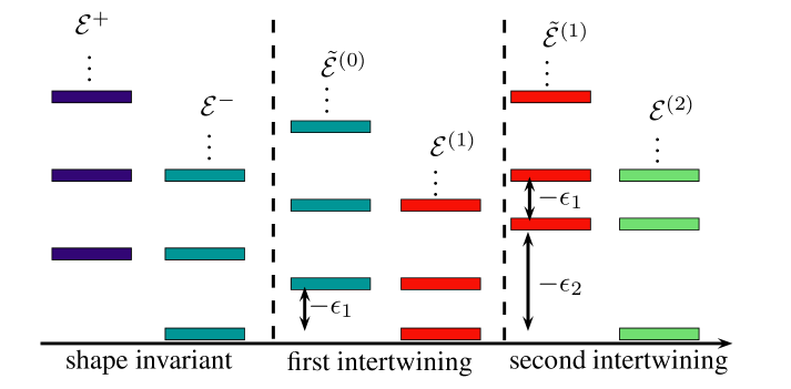
The third step of our method is to identify the eigenfunctions and eigenvalues of the new system. The energy levels for and are those of , displaced by the quantity , plus the ground state of at zero energy:
| (20) |
with . A diagram of these energies can be seen in figure 1. The unknown eigenfunctions associated to the previous energies are given by:
| (21) |
where the eigenfunctions of , and consequently those of , are assumed to be known. In addition, the ground state of fulfills the condition .
Note that a similar generalization was proposed in [29], where was displaced as in Eq.(13) instead of and it was also supposed that . However, since the non-singular first-order SUSY transformations can be implemented for factorization energies below the ground state energy of the initial Hamiltonian, for in the case addressed in [29], then the non-singular domain is really larger that the one reported there, which should include as well the interval . Moreover, the search of the general solution of the key equations (16,18) of this treatment looks simpler for the Schrödinger equation (as in this paper) than for the Riccati equation (as in [29]), although both are indeed equivalent (remember that we can go from the Riccati equation (16) to the Schrödinger equation (18) through the change , and vice versa by using ). In addition, we will see next that our approach allows to guess simply how to iterate the method in a straightforward way, which was not seen in [29].
3.2 Iteration of the method: second intertwining
Let us repeat now the steps pointed out at the previous section: in the first place a factorization energy is subtracted to the Hamiltonian :
| (22) |
such that . Thus, the ground state energy of is (see figure 1), and we denote . The intertwining relation reads:
| (23) |
with the new Hamiltonian and intertwining operators being given by:
| (24) |
The Hamiltonians , are expressed in terms of the intertwining operators as and , which leads to a pair of equations similar to (16, 17):
| (25) |
| (26) |
Once again we pass from the Riccati equation (25) to the associated Schrödinger equation through the change:
| (27) |
leading to:
| (28) |
The intertwining operator helps to find , by connecting it with the corresponding Schrödinger solution for :
| (29) |
where denotes the Wronskian of and while fulfills:
| (30) |
| (31) |
| (32) |
The eigenvalues of and are related through:
| (33) |
The unknown eigenfunctions, associated with the last eigenvalues, are:
| (34) |
where
3.3 th intertwining
For the th intertwining the same scheme is followed: the Hamiltonian is first displaced by an amount :
| (35) |
where . The intertwining relation for the th step is:
| (36) |
while the Hamiltonians , and intertwining operator are expressed as:
| (37) |
| (38) |
| (39) |
If the superpotential is expressed as , then it is obtained the following Schrödinger equation for zero factorization energy:
| (40) |
The intertwining operators supply the relation between and its predecessor, i.e., , where fulfills the Schrödinger equation:
| (41) |
By iterating these expressions for lower indices it turns out that , where
| (42) |
which allows to know all the superpotentials as well as the new potential:
| (43) |
The -order magnetic field reads now:
| (44) |
A useful form of the previous expression is also given by:
| (45) |
As previously, the eigenvalues and eigenfunctions of , must be identified. The general relation between eigenvalues is:
| (46) |
The eigenfunctions associated to the last eigenvalues are given by:
| (47) |
4 Graphene in particular magnetic fields
In this section we are going to address two known shape invariant solvable potentials, which will be achieved by assuming that the magnetic field is either constant or has an exponential decay [16, 17, 23, 29].
4.1 Constant magnetic field
The constant magnetic field is obtained from a linear vector potential , . This case leads to the well known harmonic oscillator potentials, which in terms of the superpotential are given by (9) with . Now we choose as our departure Hamiltonian:
| (48) |
whose eigenvalues and eigenfunctions are given by:
| (49) |
where , the normalization factor is and are the Hermite polinomials. The first step of the method is to move up the energy of as follows:
| (50) |
with . From the intertwining relation (14) it is obtained equation (16). The change in the last equation leads to the Schrödinger equation (18), whose general solution is:
| (51) |
with . Note that, in order to avoid singularities in the potential the parameter must be restricted to the interval . In particular, for the parameters and the superpotential becomes:
| (52) |
and the new potential reads:
| (53) |
In the variable it is obtained that:
| (54) |
which in a more compact form reads as:
| (55) |
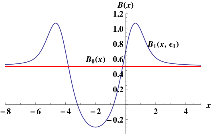
For this case the magnetic field is given by:
| (56) |
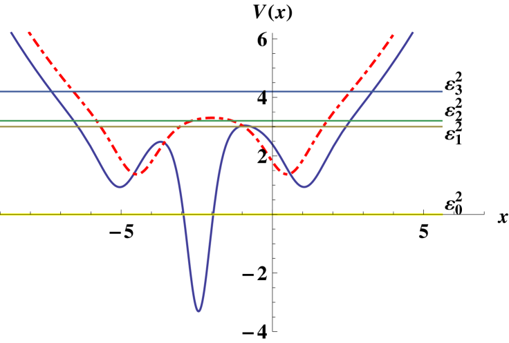
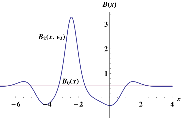
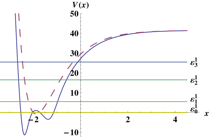
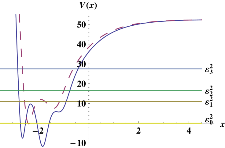
Some graphs of the potential and associated magnetic field are shown in figure 2. Since the two lowest energy levels are very close, the form of resembles the famous Mexican hat, which illustrates the spontaneous symmetry breaking in field theory. In our case the Mexican hat can be modified by changing , and its existence means that the Dirac electron can pass from the ground to the first excited state with a greater probability than for any two other states.
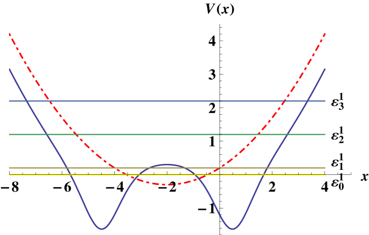
The eigenenergies of the system in our example are:
| (57) |
The corresponding eigenfunctions, taking into account (2), are given by:
| (58) |
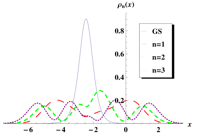
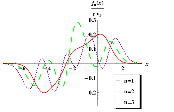
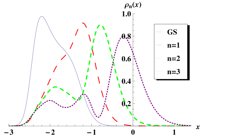
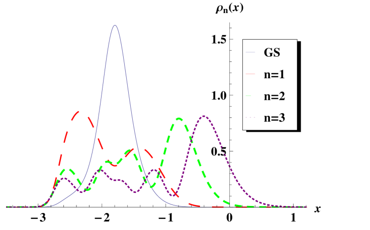
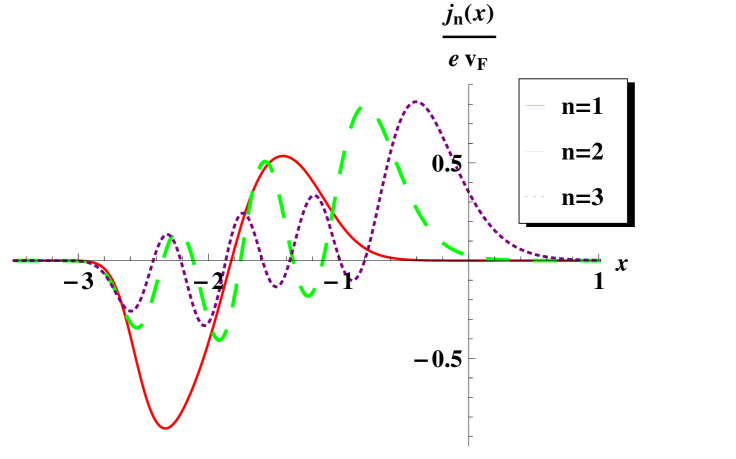
With these expressions it is customary to calculate the probability density and probability current. The probability density for the excited states of graphene is while for the ground state is . The probability currents are and respectively [23]. Some graphs for the probability density and probability current are shown in figure 3.
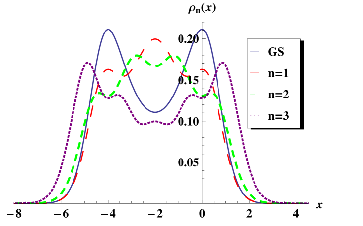
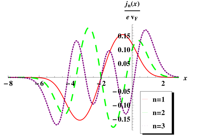
It is seen that the greater probability appears around the points where a minimum of the potential exists. Moreover, since the potential is symmetric with respect to the point , then the probability density has also the same symmetry.
4.1.1 Second-order magnetic field
In the second intertwining the potential (53) is moved up by an amount :
| (59) |
Then, it is built the second-order potential:
| (60) |
Now it is required to find the general solution of Eq. (30), which is the same of Eq. (51) but the parameter is modified to . Then we find and we build the operators for the second intertwining, . For this example we choose the particular values and . Therefore, the eigenenergies of the system become:
| (61) |
The corresponding two-component spinors are:
| (62) |
where
| (63) |
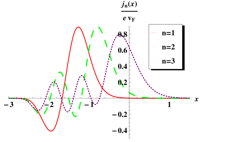
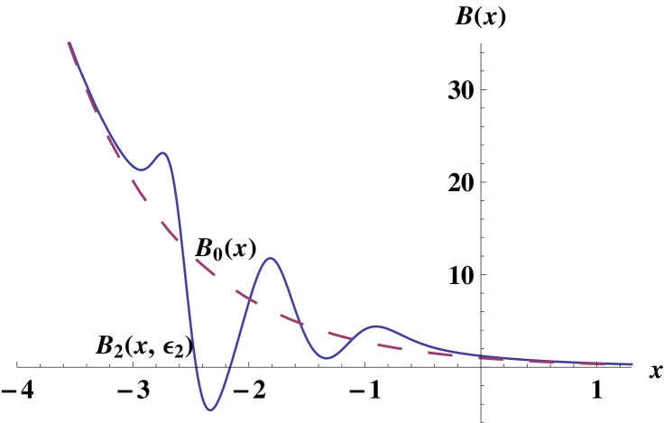
Some plots for this example are shown in figure 4, where it is drawn the second-order potential, magnetic field, probability density and current density. As in the first transformation, the shapes of the potential and magnetic field look closer to the standard parabola and horizontal line at the edges of the graphs.
Let us note that, in order to avoid singularities in , the parameter must fullfill , which is the opposite to the restriction for of the first intertwining. This choice for guarantees that none singularity will appear in the new potential .
4.2 Exponentially decaying magnetic field
In this example the vector potential reads , with , , thus the associated magnetic field becomes . The superpotential in this case is given by , , which leads to the Morse potentials:
| (64) |
We choose and displace it by to produce ; the new potential depends on , which is a solution of the Riccati Eq. (16). The new superpotential is written as , with being the general solution of the Schrödinger equation (18) given by:
| (65) |
where obeys the restriction and the parameters , are defined as:
| (66) |
Therefore, the superpotential turns out to be:
| (67) |
where the function reads:
| (68) |
The new potential and associated magnetic field are given by:
| (69) |
To illustrate these expressions we choose the factorization energy as : the corresponding plots can be observed in figure 5.

The eigenenergies for the problem are given by:
| (70) |
The eigenfunctions corresponding to take the form:
| (71) |
where is an eigenfunction of given by:
| (72) |
In this equation the normalization constant reads , while are the Laguerre polynomials, . The spinor expressions are similar to those of Eqs. (58).
Some plots for the probability and current density are shown in figure 6.
4.2.1 Second-order exponentially decaying magnetic field
This case is similar to the second intertwining for the harmonic oscillator, namely, the potential is moved up a quantity , and we choose , where is the first excited state for the Morse potential . The transformation parameters are now , and . Note that the appropriate values for are now , which is the opposite to the restriction for found in the first intertwining. The corresponding graphs for the potential, magnetic field, probability density and current density are displayed in figure 7.
5 Concluding remarks
The first-order intertwining method presented here generalizes the shape invariant technique that different authors have used previously to describe the behavior of an electron near to the Dirac points in a graphene layer with applied external magnetic fields [23, 24, 27, 28, 25, 26]. Similarly as in [29], we have modified the form of the magnetic field without destroying the exact solvability of the system, by using Schrödinger seed solutions instead of solutions for the associated Riccati equation. Once again, we recover the shape invariant results, but now in the limit . We have shown as well that the factorization energy and the parameter control the deformations induced in the initial form of the potential, magnetic field, probability density and current density.
In addition, we have introduced an iterative procedure for generating new families of higher-order potentials and magnetic fields, thus we know how to find the th-order potentials from the initial shape invariat one. The examples addressed through the second intertwining show more abrupt deformations with respect to the first transformation, but it is possible to control such deformations by appropriately choosing the four parameters , and , .
We think that it is possible in the future to develop specific models making use of the methods described in this article, for example, due to the local confinement that can be achieved through the auxiliary potentials, they could be important in electronics research. Finally, it is hoped that this work would become a guide for colleagues interested in theoretical developments of graphene.
Acknowledgments
The authors acknowledge the support of Conacyt, grant 284489. Miguel Castillo-Celeita also acknowledges the Conacyt fellowship 301117.
References
- [1] G.G. Naumis, S. Barraza-López, M. Oliva-Leyva, H. Terrones, Electronic and optical properties of strained graphene and other strained 2D materials: a review. Rev. Prog. Phys. 80, 096501 (2017).
- [2] P.R. Wallace. The Band Theory of Graphite. Phys. Rev. 71, 622 (1947).
- [3] K.S. Novoselov, A.K. Geim, S.V. Morozov, D. Jiang, Y. Zhang, S.V. Dubonos, I.V. Grigorieva, A.A. Firsov. Electric Field Effect in Atomically Thin Carbon Films. Science 306, 666 (2004).
- [4] M.I. Katsnelson. Graphene: carbon in two dimensions. Materials Today. 10, 20 (2007).
- [5] A.H. Castro Neto, F. Guinea, N.M.R. Peres, K.S. Novoselov, A.K. Geim. The electronic properties of graphene. Rev. Mod. Phys. 81, 109 (2009).
- [6] Y. Hernandez et al. High-yield production of graphene by liquid-phase exfoliation of graphite. Nat. Nanotechnol. 3, 563-568 (2008).
- [7] S. Pei and HM. Cheng. The reduction of graphene oxide. Carbon. 50, 3210-3228 (2012).
- [8] A.K. Geim and K.S. Novoselov. The rise of graphene. Nature 6, 183-191 (2007).
- [9] K.S. Novoselov, A.K. Geim, S.V. Morozov, D. Jiang, M.I. Katsnelson, I.V. Grigorieva, S.V. Dubonos, A.A. Firsov. Two-dimensional gas of massless Dirac fermions in graphene. Nature 438, 197-200 (2005).
- [10] M.I. Katsnelson, K.S. Novoselov, and A.K. Geim. Chiral tunneling and the Klein paradox in graphene. Nat. Phys. 2, 620-625 (2006).
- [11] V. Jakubský, LM. Nieto, and M.S. Plyushchay. Klein tunneling in carbon nanostructures: A free-particle dynamics in disguise. Phys. Rev. D. 83, 047702(4) (2011).
- [12] Y. Zhang, YW. Tan, H.L. Stormer and P. Kim. Experimental observation of the quantum Hall effect and Berry′s phase in graphene. Nature 438, 201-204 (2005)
- [13] J.R. Williams, L. DiCarlo, and C.M. Marcus. Quantum Hall Effect in a Gate-Controlled p-n Junction in Graphene. Science 317, 638-641 (2007).
- [14] C. Berger et al. Electronic Confinement and Coherence in Patterned Epitaxial Graphene. Science. 312, 1191-1196 (2006).
- [15] A. De Martino, L. Dell´Anna, and R. Egger. Magnetic Confinement of Massless Dirac Fermions in Graphene. Phys. Rev. Lett. 98, 066802 (2009).
- [16] G. Murguía, A. Raya, A. Sánchez and E. Reyes, The electron propagator in external electromagnetic fields in low dimensions, Am. J. Phys. 78(7), 700 (2010).
- [17] A. Raya and E. Reyes, Fermion condensate and vacuum current density induced by homogeneous and inhomogeneous magnetic fields in (2+1) dimensions, Phys. Rev. D. 82, 016004 (2010).
- [18] V. Jakubskỳ, S. Kuru, J. Negro, S. Tristao, Supersymmetry in spherical molecules and fullerenes under perpendicular magnetic fields, J. Phys.: Cond. Matt. 25, 165301 (2013).
- [19] V. Jakubský, S. Kuru, J. Negro, Carbon nanotubes in an inhomogeneous transverse magnetic field: exactly solvable model, J. Phys. A: Math. Theor. 47, 115307 (2014).
- [20] S. Kuru, J. Negro, S. Tristao, Degeneracy in carbon nanotubes under transverse magnetic delta-fields, J. Phys.: Cond. Matt. 27, 285501 (2015).
- [21] E. Díaz-Bautista and D.J. Fernández, Graphene coherent states. Eur. Phys. J. Plus. 132, 499 (2017).
- [22] M. Eshghi and H.Mehraban. Exact solution of the Dirac-Weyl equation in graphene under electric and magnetic fields. C. R. Physique 18, 47-56 (2017).
- [23] S. Kuru, J. Negro, L.M. Nieto. Exact analitic solutions for a Dirac electron moving in graphene under magnetic fields. J. Phys.: Condens. Matter. 21, 455305(11pp) (2009).
- [24] E. Milpas, M. Torres, G. Murguía, Magnetic field barriers in graphene: an analytically solvable model. J. Phys.: Cond. Matt. 23, 245304 (2011).
- [25] V. Jakubský and D. Krejčiřík. Qualitative analysis of trapped Dirac fermions in graphene. Ann. Phys. 349, 268-287 (2014).
- [26] V. Jakubský. Spectrally isomorphic Dirac systems: Graphene in an electromagnetic field. Phys. Rev. D 91, 045039 (2015).
- [27] Y. Concha, A. Huet, A. Raya, D. Valenzuela, Supersymmetric quantum electronic states in graphene under uniaxial strain, Mat.: Res. Express 5, 065607 (2018).
- [28] D. Jahani, F. Shahbazi, M.R. Setare, Magnetic dispersion of Dirac fermions in graphene under inhomogeneous field profiles, Eur. Phys. J. Plus 133, 328 (2018).
- [29] B. Midya and D.J. Fernández. Dirac electron in graphene under supersymmetry generated magnetic fields. J. Phys. A: Math. Theor. 47, 285302 (2014).
- [30] F. Cooper, A. Khare, U. Sukhatme, Supersymmetry and quantum mechanics, Phys. Rep. 251, 268-385 (1995).
- [31] B.K. Bagchi, Supersymmetry in quantum and classical mechanics, Chapman and HallCRC, Boca Raton (2000).
- [32] J.F. Cariñena and A. Ramos, Riccati equation, factorization method and shape invariance, Rev. Math. Phys. 12, 1279-1304 (2000).
- [33] A. Andrianov, F. Cannata, M. Ioffe, D. Nishnianidze, System with higher-order shape invariance: spectral and algebraic properties, Phys. Lett. A 266, 341-349 (2000).
- [34] D.J. Fernández, Supersymmetric quantum mechanics, AIP Conf. Proc. 1287, 3-36 (2010).
- [35] D.J. Fernández, Trends in supersymmetric quantum mechanics, Integrability, supersymmetry and coherent states, CMR Series, S. Kuru et al. (eds.), Springer Nature Switzerland AG (2019), to be published.
- [36] D.J. Fernández and V. Hussin, Higher-order SUSY, linearized non-linear Heisenberg algebras and coherent states, J. Phys. A: Math. Gen. 32, 3603-3619 (1999).
- [37] D.J. Fernández and N. Fernández-García, Higher-order supersymmetric quantum mechanics, AIP Conf. Proc. 744, 236-273 (2005).