Direct Measurement of the Quantum Wavefunction
Abstract
Central to quantum theory, the wavefunction is the complex distribution used to completely describe a quantum system. Despite its fundamental role, it is typically introduced as an abstract element of the theory with no explicit definition Cohen-Tannoudji2006 ; Mermin2009 . Rather, physicists come to a working understanding of the wavefunction through its use to calculate measurement outcome probabilities via the Born Rule Landau1989 . Presently, scientists determine the wavefunction through tomographic methods Vogel1989 ; Smithey1993 ; Breitenbach1997 ; White1999 ; Hofheinz2009 , which estimate the wavefunction that is most consistent with a diverse collection of measurements. The indirectness of these methods compounds the problem of defining the wavefunction. Here we show that the wavefunction can be measured directly by the sequential measurement of two complementary variables of the system. The crux of our method is that the first measurement is performed in a gentle way (i.e. weak measurement Aharonov1988 ; Ritchie1991 ; Resch2004 ; Smith2004 ; Pryde2005 ; Mir2007 ; Hosten2008 ; Dixon2009 ; Lundeen2009 ; Aharonov2010 ) so as not to invalidate the second. The result is that the real and imaginary components of the wavefunction appear directly on our measurement apparatus. We give an experimental example by directly measuring the transverse spatial wavefunction of a single photon, a task not previously realized by any method. We show that the concept is universal, being applicable both to other degrees of freedom of the photon (e.g. polarization, frequency, etc.) and to other quantum systems (e.g. electron spin-z quantum state, SQUIDs, trapped ions, etc.). Consequently, this method gives the wavefunction a straightforward and general definition in terms of a specific set of experimental operations Bridgman1927 . We expect it to expand the range of quantum systems scientists are able to characterize and initiate new avenues to understand fundamental quantum theory.
The wavefunction , also known as the ‘quantum state’, is considerably more difficult to measure than the state of a classical particle, which is determined simply by measuring its position and momentum . According to the Heisenberg Uncertainty Principle, in quantum theory a precise measurement of disturbs the particle’s wavefunction and forces a subsequent measurement of to become random. Thus we learn nothing of the particle’s momentum. Indeed, it is impossible to determine a completely unknown wavefunction of single system Wootters1982 .
Consider instead performing a measurement of on an ensemble of particles, all with the same . The probability of getting result is . Similarly, the probability of would be , where is the Fourier transform of Even these two probability distributions are not enough to determine unambiguously (see the 1d phase retrieval problem Trebino2002 ). Instead, one must reconstruct by performing a large set of distinct measurements (e.g. ), and then estimating a that is most compatible with the measurement results. This method is known as quantum state tomography Vogel1989 ; Smithey1993 ; Breitenbach1997 ; White1999 ; Hofheinz2009 . In contrast, we introduce a method to measure of an ensemble directly. Here, by ‘direct’ we mean that the method is free from complicated sets of measurements and computations; the average raw signal originating from where the wavefunction is being probed is simply proportional to its real and imaginary components at that point. The method rests upon the sequential measurement of two complementary variables of the system.
At the center of the direct measurement method is a reduction to the disturbance induced by the first measurement. Consider the measurement of an arbitrary variable . In general, measurement can be seen as the coupling between an apparatus and a physical system that results in the translation of a pointer. The pointer position indicates the result of a measurement. In a technique known as ‘weak measurement’, one reduces the coupling strength and this correspondingly reduces the disturbance created by the measurement Aharonov1988 ; Ritchie1991 ; Resch2004 ; Smith2004 ; Pryde2005 ; Mir2007 ; Hosten2008 ; Dixon2009 ; Lundeen2009 ; Aharonov2010 . This strategy also compromises measurement precision but this can be regained by averaging. The average of the weak measurement is simply the expectation value , indicated by an average position shift of the pointer proportional to this amount.
A distinguishing feature of weak measurement is that it does not disturb a subsequent normal (or ‘strong’) measurement of another observable in the limit where the coupling vanishes. For the particular ensemble subset that gave outcome one can derive the average of the weak measurement of . In the limit of zero interaction strength, this is called the Weak Value and is given Aharonov1988 by,
| (1) |
Selecting a particular subset of an ensemble based on a subsequent measurement outcome is known as ‘post-selection’, and is a common tool in quantum information processing Knill2001 ; Duan2001 .
Unlike the standard expectation value , the Weak Value can be a complex number. This seemingly strange result can be shown to have a simple physical manifestation: the pointer’s position is shifted by Re and receives a momentum kick of Im Aharonov1990 ; Lundeen2005 ; Jozsa2007 . The complex nature of the Weak Value suggests that it could be used to indicate both the real and imaginary parts of the wavefunction.
Returning to our example of a single particle, consider the weak measurement of position () followed by a strong measurement of momentum giving . In this case the Weak Value is
| (2) | ||||
| (3) |
In the case , this simplifies to
| (4) |
where is a constant (which can be eliminated later by normalizing the wavefunction). The average result of the weak measurement of is proportional to the wavefunction of the particle at . Scanning the weak measurement through gives the complete wavefunction. At each , the observed position and momentum shifts of the measurement pointer are proportional to Re and Im , respectively. In short, by reducing the disturbance induced by measuring and then measuring normally, we measure the wavefunction of the single particle.
As an experimental example, we performed a direct measurement of the transverse spatial wavefunction of a photon. Considering a photon travelling along the direction, we directly measure the wavefunction of the photon, sometimes called the ‘spatial mode’ (see the Supplementary Discussion). The Wigner function of the spatial mode of a classical beam has been measured directly but not for a single photon state Mukamel2003 ; Smith2005 .
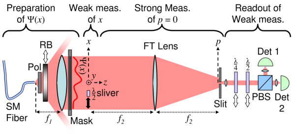
We produce a stream of photons in one of two ways, either by attenuating a laser beam or by generating single photons through spontaneous parametric downconversion (SPDC) (see the Supplementary Methods for details). The photons have a center wavelength of nm or nm, respectively. The experiment (details and schematic in Fig. 1) can be divided into four sequential steps: preparation of the transverse wavefunction, weak measurement of the transverse position of the photon, post-selection of those photons with zero transverse momenta, and readout of the weak measurement.
An ensemble of photons with wavefunction is emitted from a single mode (SM) fiber and collimated. We will begin by directly measuring this wavefunction (described in detail in Fig. 1). We then further test our method by inducing known magnitude and phase changes to the photons here to prepare a series of modified wavefunctions.
We weakly measure the transverse position of the photon by coupling it to an internal degree of freedom of the photon, its polarization. This allows us to use the linear polarization angle of the photon as the pointer. At a position where we wish to measure we rotate the linear polarization of the light by Consider if is set to . In this case, one can perfectly discriminate whether a photon had position because it is possible to perfectly discriminate between orthogonal polarizations, and . This is a strong measurement. Reducing the strength of the measurement corresponds to reducing , which makes it impossible to discriminate with certainty whether any particular photon had The benefit of this reduction in precision is a commensurate reduction in the disturbance to the wavefunction of the single photon.
We then use a Fourier Transform lens and a slit to post-select only those photons with . This constitutes the strong measurement of .
In this subset of the photon ensemble, we find the average value of our weak measurement of . The average rotation of the pointer, the linear polarization, is proportional to the real part of the Weak Value. Its complementary pointer variable, the rotation in the circular polarization basis, is proportional to the imaginary part of the Weak Value Lundeen2005 . Formally, if we treat the initial polarization as a spin-1/2 spin down vector, then the weak value is given by
| (5) |
where and are the Pauli x and y matrices, respectively, and is the final polarization state of the pointer Lundeen2005 . We measure the and expectation values by sending the photons through either through a half-wave plate or quarter-wave plate, respectively, and then through a polarizing beamsplitter (PBS). Thus, we read out Re (half-wave plate) and Im (quarter-wave plate) from the signal imbalance between detectors 1 and 2 at the outputs of the PBS.
With , we scan our measurement of in 1 mm steps and find the Weak Value at each step. In this way, we directly measure the photon transverse wavefunction, . We normalize the and measurements by the same factor, so that which eliminates the proportionality constant,
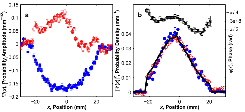
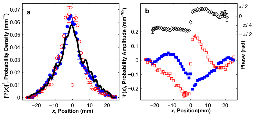
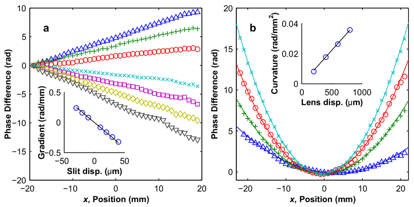
To confirm our direct measurement method, we test it on a series of different wavefunctions. Using our SPDC single photon source, we start by measuring the initial truncated Gaussian wavefunction (Fig. 2) described in Fig. 1. Switching to the laser source of photons, we then modify the magnitude, and then the phase, of the initial wavefunction with an apodized filter and glass plate, respectively, to create two new test (Fig. 3). We conduct more quantitative modification of the wavefunction phase by introducing a series of phase gradients and then phase curvatures (Fig. 4). For all the test wavefunctions, we have found good agreement between the expected and measured wavefunction, including its phase and magnitude (see the Figure Captions for details).
We now describe how the technique of weak measurement can be used to directly measure the quantum state of an arbitrary quantum system. We have the freedom to measure the quantum state in any chosen basis (associated with observable ) of the system. The method entails weakly measuring a projector in this basis, e.g. , and post-selecting on a particular value of the complementary observable (See the Supplementary Discussion for a precise definition of complementarity). In this case, the Weak Value is
| (6) |
where is a constant, independent of . Thus the Weak Value is proportional to the amplitude of state in the quantum state. Stepping through all the states in the basis directly gives the quantum state represented in that basis
| (7) |
This is the general theoretical result of this paper. It shows that in any physical system one can directly measure the quantum state of that system by scanning a weak measurement through a basis and appropriately post-selecting in the complementary basis.
Weak measurement necessarily trades efficiency for accuracy or precision. A comparison of our method to current tomographic reconstruction techniques will require careful consideration of the signal to noise ratio in a given system. In order to increase this ratio in the direct measurement of the photon spatial wavefunction, future experiments will investigate the simultaneous post-selection of many transverse momenta.
In our direct measurement method, the wavefunction manifests itself as shifts of the pointer of the measurement apparatus. In this sense, the method provides a simple and unambiguous Operational definition Bridgman1927 of the quantum state: it is the average result of a weak measurement of a variable followed by a strong measurement of the complementary variable. We anticipate that the simplicity of the method will make feasible the full characterization of quantum systems (e.g. atomic orbitals, molecular wavefunctions Itatani2004 , ultrafast quantum wavepackets Dudovich2006 ) previously unamenable to it. The method can also be viewed as a transcription of quantum state of the system to that of the pointer, a potentially useful protocol for quantum information.
Acknowledgements.
This work was supported by the Natural Sciences and Engineering Research Council and the Business Development Bank of Canada. The concept and theory was by J.S.L. All authors contributed to the design and building of the experiment and the text of the manuscript. J.S.L, B.S. and C.B. performed the measurements and data analysis. Reprints and permissions information is available at www.nature.com/reprints. The authors declare no competing financial interests. Readers are weclome to comment on the online version of this article at www.nature.com/nature. Correspondence and requests for materials should be addressed to J.S.L. (jeff.lundeen@nrc-cnrc.gc.ca).References
- (1)
- (2) Cohen-Tannoudji, C., Diu, B. & Laloe, F. Quantum Mechanics, vol. 1, 19 (Wiley-Interscience, 2006).
- (3) Mermin, N. D. What’s bad about this habit. Phys. Today 62, 8–9 (2009).
- (4) Landau, L. D. & Lifshitz, E. M. Quantum Mechanics: Non-relativistic theory, vol. 3 of Course of Theoretical Physics, 6 (Pergamon Press, Oxford; New York, 1989), third edn.
- (5) Vogel, K. & Risken, H. Determination of quasiprobability distributions in terms of probability distributions for the rotated quadrature phase. Phys. Rev. A 40, 2847–2849 (1989).
- (6) Smithey, D. T., Beck, M., Raymer, M. G. & Faridani, A. Measurement of the wigner distribution and the density matrix of a light mode using optical homodyne tomography: Application to squeezed states and the vacuum. Phys. Rev. Lett. 70, 1244–1247 (1993).
- (7) Breitenbach, G., Schiller, S. & Mlynek, J. Measurement of the quantum states of squeezed light. Nature 387, 471–475 (1997).
- (8) White, A. G., James, D. F. V., Eberhard, P. H. & Kwiat, P. G. Nonmaximally entangled states: Production, characterization, and utilization. Phys. Rev. Lett. 83, 3103–3107 (1999).
- (9) Hofheinz, M. et al. Synthesizing arbitrary quantum states in a superconducting resonator. Nature 459, 546–549 (2009).
- (10) Aharonov, Y., Albert, D. Z. & Vaidman, L. How the result of a measurement of a component of the spin of a spin-1/2 particle can turn out to be 100. Phys. Rev. Lett. 60, 1351–1354 (1988).
- (11) Ritchie, N. W. M., Story, J. G. & Hulet, R. G. Realization of a measurement of a “weak value”. Phys. Rev. Lett. 66, 1107–1110 (1991).
- (12) Resch, K. J., Lundeen, J. S. & Steinberg, A. M. Experimental realization of the quantum box problem. Phys. Lett. A 324, 125–131 (2004).
- (13) Smith, G. A., Chaudhury, S., Silberfarb, A., Deutsch, I. H. & Jessen, P. S. Continuous weak measurement and nonlinear dynamics in a cold spin ensemble. Phys. Rev. Lett. 93, 163602 (2004).
- (14) Pryde, G. J., O’Brien, J. L., White, A. G., Ralph, T. C. & Wiseman, H. M. Measurement of quantum weak values of photon polarization. Phys. Rev. Lett. 94, 220405 (2005).
- (15) Mir, R. et al. A double-slit ’which-way’ experiment on the complementarity-uncertainty debate. New J. Phys. 9, 287 (2007).
- (16) Hosten, O. & Kwiat, P. Observation of the spin hall effect of light via weak measurements. Science 319, 787–790 (2008).
- (17) Dixon, P. B., Starling, D. J., Jordan, A. N. & Howell, J. C. Ultrasensitive beam deflection measurement via interferometric weak value amplification. Phys. Rev. Lett. 102, 173601 (2009).
- (18) Lundeen, J. S. & Steinberg, A. M. Experimental joint weak measurement on a photon pair as a probe of hardy’s paradox. Phys. Rev. Lett. 102, 020404 (2009).
- (19) Aharonov, Y., Popescu, S. & Tollaksen, J. A time-symmetric formulation of quantum mechanics. Physics Today 63, 27–32 (2010).
- (20) Bridgman, P. The Logic of Modern Physics (New York: Macmillan, 1927).
- (21) Wootters, W. K. & Zurek, W. H. A single quantum cannot be cloned. Nature 299, 802–803 (1982).
- (22) Trebino, R. Frequency-Resolved Optical Gating: The Measurement of Ultrashort Laser Pulses (Springer, New York, NY, 2002).
- (23) Knill, E., Laflamme, R. & Milburn, G. J. A scheme for efficient quantum computation with linear optics. Nature 409, 46–52 (2001).
- (24) Duan, L. M., Lukin, M. D., Cirac, J. I. & Zoller, P. Long-distance quantum communication with atomic ensembles and linear optics. Nature 414, 413–418 (2001).
- (25) Aharonov, Y. & Vaidman, L. Properties of a quantum system during the time interval between two measurements. Phys. Rev. A 41, 11–20 (1990).
- (26) Lundeen, J. S. & Resch, K. J. Practical measurement of joint weak values and their connection to the annihilation operator. Phys. Lett. A 334, 337–344 (2005).
- (27) Jozsa, R. Complex weak values in quantum measurement. Phys. Rev. A 76, 044103 (2007).
- (28) Mukamel, E., Banaszek, K., Walmsley, I. A. & Dorrer, C. Direct measurement of the spatial wigner function with area-integrated detection. Opt. Lett. 28, 1317–1319 (2003).
- (29) Smith, B. J., Killett, B., Raymer, M. G., Walmsley, I. A. & Banaszek, K. Measurement of the transverse spatial quantum state of light at the single-photon level. Opt. Lett. 30, 3365–3367 (2005).
- (30) Itatani, J. et al. Tomographic imaging of molecular orbitals. Nature 432, 867–871 (2004).
- (31) Dudovich, N. et al. Measuring and controlling the birth of attosecond xuv pulses. Nature Phys. 2, 781–786 (2006).
I Supplementary Methods
I.1 Single Photon Source
In this section, we describe how we produce a stream of single photons. A mode-locked Ti:Sapphire laser produces 100 fs FWHM pulses of light centered on a wavelength of 800nm (Newport Mai-Tai HP). The pulses are frequency doubled in a 1mm long BBO crystal cut for Type I collinear phase-matching to have a wavelength of 400nm. The 800nm red light is reflected away with dielectric dichroic filters and the 400nm light is focused on a 0.3 mm long BBO cut for Type II collinear phase-matching. Through spontaneous parametric downconversion, pairs of collinear photons having a center wavelength of nm are produced in the crystals. One photon is horizontally polarized (H) and the other is vertically polarized (V). Although they are produced rarely, since they are always produced in pairs the presence of one photon can be used to ‘herald’ the presence of its twin. We split the photon pair into two separate beams with a polarizing beamsplitter (PBS). We couple the H photon into a multimode fiber which leads to a single photon detector (Silicon Avalanche Photodiodes, PerkinElmer SPCM-AQHR-13). A click at this detector then heralds the presence of the V photon in the other beam, thus producing a single photon state of light. The V photon is the subject of the measurements we describe in the main article.
I.2 Laser Source
In this section we give details of our laser source of photons. We use a diode laser that produces continuous wave light at nm as a brighter source of photons with which to test our direct measurement method. We temperature stabilize the diode to prevent drifts in its wavelength. The emitted photons are sent through a polarizer and then coupled into a single mode polarization maintaining fiber, which we couple to the initial single mode fiber in our experiment.
I.3 Waveplate Sliver Details
In addition to the polarization rotation, the waveplate sliver generates two unwanted transformations in the measured photons, a large shift and a phase-shift. Tilting the waveplate sliver about the axis allows us to null the induced phase-shift. We precompensate for the shift before the fiber in the following way. Because the photon is fairly broadband (10nm), its coherence length is short (30 um). The waveplate sliver (mm thick) described in the main paper displaces the photon by , where is the optical index. This displacement is longer than the photon’s coherence length. If displaced beyond one coherence length, the photon will not exhibit the required interference between the amplitude for a photon to go through the sliver and the amplitude to go around it. Therefore we precompensate for this by first creating two amplitudes for the single photon separated by exactly the displacement created by waveplate sliver. We achieve this exactness by using another piece of the waveplate the from which the sliver was cut. By placing this extra piece of waveplate so that it covers half of the vertically polarized beam emerging from the PBS and then coupling that beam into a single-mode polarization maintaining optical fiber (Nufern PM780-HP), we create the two amplitudes, and . We measure the wavefunction of the photons emerging from the other end of this fiber.
Propagating these two amplitudes through the waveplate sliver, we have and whereas the amplitudes to go around the sliver will remain and . The amplitudes from each process will interfere, whereas the and , being orthogonal, will not. The latter amplitudes simply add a constant background to our measurement of and halving the magnitude of and Nonetheless the proportionality to remains and this decrease in signal is inconsequential after normalizing
II Supplementary Discussion
II.1 The Transverse Photon Wavefunction
The total quantum state of the photon is a function of the photon’s polarization and the three spatial degrees of freedom, , , and . If there are no correlations between these four degrees of freedom, one can write the total wavefunction of the photon as a product of wavefunctions, one for each degree of freedom. Under these conditions, one can measure the wavefunction of each degree of freedom separately. Considering a photon travelling along the direction, we directly measure the wavefunction of the photon.
There are techniques for measuring the spatial mode of a classical beam of light. These include spatial-shear interferometry, Shack-Hartman sensors Platt2001 (31), spiral interferometry Juanola-Parramon2008 (32), the Gerchberg-Saxton algorithm Gerchberg1972 (33), and conoscopic holography Buse2000 (34). Some of these might be applicable to single photons. However, none of these techniques are direct, either measuring only phase gradients or and stitching these together to estimate the actual phase , or requiring computer algorithms to interpret the results.
II.2 Complementarity
Central to this method is the concept of complementarity, which is formalized by the theory of Mutually Unbiased (MU) Bases Durt2010 (35). Two bases and are MU if all their constituent states have the same overlap, i.e. for any values of and , where is the dimension of the Hilbert space. A strong measurement of will leave the system in a flat distribution of the basis. In any physical system there are always at least two bases that are mutually unbiased. By unitary transformation, once one of the bases in the MU pair is selected, the other is then fixed. Thus we are free to choose our basis for the direct measurement of the quantum state (i.e. we are guaranteed there will be at least one variable that we can post-select on). In every basis that is unbiased with respect to our direct measurement basis, there is a state for which is a constant, i.e. the phase of the overlap is independent of Durt2010 (35). Post-selecting on this state will result in a weak value that that is proportional to the quantum state. The proportionality constant, , is a constant, independent of .
The choice of state to post-select on is in fact somewhat arbitrary. Any state in can be used. Now, the stipulation thatis a constant sets the laboratory reference frame relative to which is measured. In the measurement of the photon transverse wavefunction, momentum is defined relative to a lab coordinate system set by an axis joining the center of the Fourier Transform lens to the slit. One is thus free to set to be whatever direction one chooses; the wavefunction will be measured relative to this coordinate frame.
The theory of MU bases is less developed for continuous variables such as those in our example, and of a single particle. In a Hilbert space defined by an unbounded continuous variables such as these, for any chosen variable then will be respectively unbiased for any ; there exist an infinite number of MU pairs of bases Weigert2008 (36). Theoretically, this creates a great deal of flexibility in the method to directly measure the wavefunction. In practice though, basis states of continuous variables are not physical, in that the range of in projector is zero, For a finite range measurement, , the associated states are no longer mutually unbiased. In this case, the most unbiased pair of bases will be and e.g. and .
References
- (1) Platt, B. C. & Shack, R. History and principles of shack-hartmann wavefront sensing. J. Refract. Surg. 17, S573–S577 (2001).
- (2) Juanola-Parramon, R., Gonzalez, N. & Molina-Terriza, G. Characterization of optical beams with spiral phase interferometry. Opt. Express 16, 4471–4478 (2008).
- (3) Gerchberg, R. W. & Saxton, W. O. A practical algorithm for the determination of the phase from image and diffraction plane pictures. Optik 35, 237 (1972).
- (4) Buse, K. & Luennemann, M. 3d imaging: Wave front sensing utilizing a birefringent crystal. Phys. Rev. Lett. 85, 3385–3387 (2000).
- (5) Durt, T., Englert, B., Bengtsson, I. & Zyczkowski, K. On mutually unbiased bases. ArXiv e-prints (2010). eprint 1004.3348.
- (6) Weigert, S. & Wilkinson, M. Mutually unbiased bases for continuous variables. Phys. Rev. A 78, 020303 (2008).