Discontinuous eikonal equations
in metric measure spaces
Abstract.
In this paper, we study the eikonal equation in metric measure spaces, where the inhomogeneous term is allowed to be discontinuous, unbounded and merely -integrable in the domain with a finite . For continuous eikonal equations, it is known that the notion of Monge solutions is equivalent to the standard definition of viscosity solutions. Generalizing the notion of Monge solutions in our setting, we establish uniqueness and existence results for the associated Dirichlet boundary problem. The key in our approach is to adopt a new metric, based on the optimal control interpretation, which integrates the discontinuous term and converts the eikonal equation to a standard continuous form. We also discuss the Hölder continuity of the unique solution with respect to the original metric under regularity assumptions on the space and the inhomogeneous term.
Key words and phrases:
eikonal equation, metric spaces, discontinuous inhomogeneous term, viscosity solutions2010 Mathematics Subject Classification:
35R15, 49L25, 35F30, 35D401. Introduction
1.1. Background and motivation
In this paper we study the eikonal equation in a metric measure space with a possibly discontinuous inhomogenous term, where is assumed to be a nonnegative, locally finite Borel measure. We assume that is a complete length space and is a bounded domain. We consider
| (1.1) |
with the Dirichlet boundary condition
| (1.2) |
where is a given positive Borel measurable function in and is a given bounded function on . Further assumptions on and will be introduced later.
Well-posedness of the eikonal equation and more general Hamilton-Jacobi equations is a classical topic. The theory of viscosity solutions provides a successful tool to solve such fully nonlinear PDEs in the Euclidean space. It is well known that when and satisfies the lower bound condition
| (1.3) |
there exists a unique viscosity solution of (1.1) with Dirichlet data (1.2) under appropriate regularity condition on . The uniqueness result is obtained by establishing a comparison principle while the existence of solutions can be proved via several different approaches including Perron’s method and a control-based formula.
Let us give more details on the connection with the optimal control theory, as it largely motivates our exploration and plays a central role in this work. It is widely known [40, 6] that, under appropriate conditions on and , the unique viscosity solution of (1.1) with the Dirichlet boundary condition (1.2) in the Euclidean space can be expressed by
| (1.4) |
This formula represents the so-called value function of an optimal control problem, where one tries to move a point from toward the boundary and minimize the total payoff comprising a running cost integrated along the trajectory and a terminal cost at the first hit on the boundary. See [38, 31] and references therein for more recent developments on representation formulas for general Hamilton-Jacobi equations.
The representation formula not only provides a clear understanding of the solution and promotes various control-related practical applications, but also suggests possible generalization of the theory for a possibly discontinuous function . In fact, much progress has been made in this direction in the Euclidean space. The study on discontinuous Hamilton-Jacobi equations in the Euclidean space was initiated in the work [36] and later found applications in geometric optics with different layers, image processing, shape from shading, etc. Further development in different contexts to treat discontinuous Hamiltonians including the time-dependent case can be found in [55, 47, 48, 53, 12, 11, 19, 8, 13, 54, 17, 27, 28]. The aforementioned papers in the Euclidean case, reduced to our eikonal problem, seem to need at least local essential boundedness of for their well-posedness results except for the papers [55, 53, 54]. In these three papers, the results regarding uniqueness and existence results rely on regularity conditions on the discontinuity set of or certain controllability assumptions for the optimal control formulation. Such conditions can hardly be extended further to our relaxed geometric setting due to the lack of smooth structure in general metric spaces.
In the present paper we aim to study in a direct manner the eikonal equation with potentially wilder discontinuity than those considered in [55, 53, 54]. We drop the local boundedness of the inhomogeneous data and allow it to be as discontinuous as a function in . It is worth adding that an important tool called viscosity solution theory has been developed for second order uniformly elliptic equations with measurable data in [10, 18], but it does not seem to apply to the first order case. For the Dirichlet problem (1.1)(1.2), our primary observation is that the formula (1.4) actually requires nothing more than the path integrability of along a curve connecting to the boundary, which is a much weaker assumption than the continuity or even boundedness of . Let us present a simple one-dimensional example to clarify this point.
Let and set such that
| (1.5) |
The value can be chosen to be any positive real number in order to meet the requirement (1.3). Such type of singular eikonal equations finds applications in lens design for wireless communication systems [16]. It is clear that with . Therefore the formula in (1.4) still makes sense for given boundary data at . For instance, setting , we see that the formula immediately yields
| (1.6) |
It seems to be the correct solution of (1.1)(1.2), for it satisfies the standard definition of viscosity solutions if we consider . Also, one can verify the validity of approximation via truncation of the running cost. Indeed, taking for large, we can obtain a unique viscosity solution for the truncated problem with the bounded function . By direct calculations, we easily see that the approximate solution converges uniformly to in . Moreover, although in general we cannot expect Lipschitz regularity of solutions due to the loss of boundness of , the example shows that the solution enjoys Hölder regularity that depends on the integrability of . This can be viewed as a natural consequence corresponding to the Morrey-Sobolev inequality, as the eikonal equation suggests at least formally.
To the best of our knowledge, the well-posedness and regularity issue for this type of discontinuous eikonal equations have not been carefully examined even in the Euclidean case. We are therefore motivated to tackle these problems in a general way that permits applications to a broad class of metric measure spaces with length structure. We develop the notion of Monge solutions used in [47, 8, 43] and show uniqueness and existence of solutions in this general setting. We also establish Hölder regularity of the solution under certain regularity assumptions on and . More details about our results will be given momentarily.
First-order Hamilton-Jacobi equations in metric spaces have recently attracted great attention for applications in optimal transport [5, 57], mean field games [14], topological networks [49, 35, 1, 33, 34] etc. Concerning the equations that depend on the gradient in terms of its norm, we refer to [4, 29, 26, 45] for several different notions of viscosity solutions as well as the associated uniqueness and existence results. In our previous paper [43], we proved the equivalence of these solutions and introduce another alternative notion, extending the approach of Monge solutions proposed in [47] to the eikonal equation in complete length spaces; see also an application of this Monge-type notion to the study of the first eigenvalue problem for the infinity Laplacian in metric spaces [41]. Our current work further develops the notion of Monge solutions so that viscosity solution theory will be available to handle a class of nonlinear equations in general metric measure spaces with data having a wider range of discontinuities.
Our work is new even from the point of view of pure analysis. There has been great progress on various aspects of first order analysis on metric measure spaces, including first order Sobolev spaces and their relation to variational problems and partial differential equations. One central notion that generalizes the norm of the gradient of a Sobolev function in Euclidean spaces is the so-called upper gradient. We refer the reader to [30] for a survey of the Sobolev spaces theory built upon this notion. From this point of view, the Dirichlet problem (1.1) with boundary data (1.2) can be interpreted as an extension problem for a function to with boundary value assigned on and the upper gradient prescribed in . In general, many possible choices can be expected, among which the viscosity solution constructed by the formula (1.4) is usually considered to be the most “physical”. This perspective can also be found in the work [15]. There is certainly no need to restrict the prescribed gradient to a continuous or bounded function class. We are thus inspired to address the extension problem for and investigate properties of the extended function .
1.2. General results on existence and uniqueness of solutions
Our presentation can be divided into two parts. The first part, consisting of Sections 2–4, is a general PDE theory with only the length structure and curve-wise integrals of involved. In our main well-posedness results, we impose certain key conditions on the closure of the domain and the inhomogeneous term . In the second part, adding a measure structure to the space, we provide more specific sufficient conditions for those assumptions on and .
One of the crucial steps in the first part is to find an appropriate notion of viscosity solutions in this setting that agrees with the representation formula (1.4) and justifies a comparison principle for us to prove the uniqueness. As mentioned above, we adopt the notion of Monge solutions, which in the case of a continuous , requires
| (1.7) |
where, for a locally Lipschitz function , the subslope is defined by
In the Euclidean space, this definition is known to be equivalent to the usual viscosity solutions [47]. One of its advantages is that it avoids using smooth test functions, whose lack of availability is indeed a key difficulty in the study of Hamilton-Jacobi equations in general metric spaces.
When is of class , the definition in (1.7) may not apply directly. For example, if one changes the value of to be finite in the aforementioned example, then the expected solution (1.6) does not satisfy definition (1.7) at . We thus need to somehow exploit collective information of rather than its pointwise value. Also, we always assume that the lower bound condition (1.3) holds for in order to obtain uniqueness. Heuristically speaking, since is uniformly positive in , we can rewrite the equation (1.1) as
and adopt a new pointwise slope by incorporating the value of into the metric. This approach enables us to study the eikonal equation as if the right hand side is a constant. Such connection can be rigorously realized by introducing the following new metric, which is also called optical length function in [47, 8] etc.,
| (1.8) |
where denotes the collection of all curves connecting and in on which the path integral is finite, namely,
We say that the curves in are admissible with respect to . We shall assume throughout Sections 2–4 that
| (1.9) |
so that the formula in (1.4) is well defined for any . In Section 5, we discuss some sufficient assumptions on implying (1.9).
Adopting the subslope with respect to this newly defined metric , defined by
| (1.10) |
one can simply define the Monge solution of (1.1) in Definition 3.1 by asking that satisfies
| (1.11) |
The same idea of changing metrics was also outlined in [9] in connection with metric geometry and in [56] for applications in homogenization.
This new definition of Monge solutions is consistent with the well-studied case where is continuous. In fact, if is continuous at , then
| (1.12) |
It is then easily seen that and are equivalent.
Switching the metric from to enables us to reduce the possibly discontinuous inhomogeneous data in (1.7) to the continuous standard form (1.11). As a consequence, most of our arguments in [43] can be applied to establish the comparison principle and prove existence of solutions of (1.1), (1.2) under the compatibility condition
| (1.13) |
However, a major challenge concerning the topological change of the space appears in the proof of comparison principle. Note that the metrics and are not topologically equivalent in general, especially when is unbounded. One can find examples where fails to imply ; see Example 2.4. For most of our analysis, we impose the following key compatibility condition
| (1.14) |
which ensures that the topology induced by is in agreement with the metric topology inherited from , and enables us to obtain not only the uniqueness but also the uniform continuity of Monge solutions.
In general, if (1.14) fails to hold, then, because of the change in the metric, the domain that is bounded in may become unbounded in . The notions of interior and boundary points of may also change accordingly. However, it is still possible to show uniqueness and existence of Monge solutions if we have boundedness of with respect to as well as a weaker version of (1.14) as below:
| (1.15) |
where . Here, we denote . In this case, we can get a unique Monge solution that is Lipschitz continuous in but possibly discontinuous in ; see Example 4.4 for a concrete example. Note that the completeness of is preserved under our metric change (Lemma 2.5), which enables us to establish a comparison principle based on Ekeland’s variational principle.
Our main result can be summarized as follows. Its proof is given in Section 4.
Theorem 1.1 (Existence and uniqueness of solutions).
Let be a complete length space and be a bounded domain. Assume that (1.3) and (1.9) hold. Let be given by (1.8), and be bounded. Consider the function defined by
| (1.16) |
Then the following results hold.
-
(i)
is Lipschitz in with respect to and is a Monge solution of (1.1).
- (ii)
- (iii)
The interpretation (1.17) is automatically guaranteed by (1.2) if is assumed to be compact. Our comparison results with and without compactness of are presented in Section 3.2. We also include a discussion in Section 4.2 about the case when the compatibility condition (1.13) on fails to hold. In the Euclidean space, this corresponds to loss of Dirichlet boundary data, and one needs to relax the boundary condition in the viscosity sense; see for example [51, 52, 37] for the well-posedness results under certain regularity conditions on . Thanks to the general setting considered in this present paper, we treat this problem in a more direct way. If the boundary data on a part of is lost, we take the remaining piece, denoted by , as the real boundary and regard as the interior of the domain. In fact, the formula (1.4) does yield the Monge solution property of in . Such flexibility in changing the notion of boundary and interior points leads us to uniqueness and existence of solutions to the reduced Dirichlet problem.
1.3. Regularity of solutions and further discussions
The second half of our presentation is devoted to understanding more deeply the key assumptions (1.9) and (1.14) in Theorem 1.1. We study this regularity problem in the setting of a general metric measure space with the measure assumed to be doubling. We recall that a locally finite Borel measure is doubling if there exists such that for all , where denotes the open metric ball centered at with radius , i.e.,
We also call the homogeneous dimension of the doubling metric measure space. It is not difficult to see that by the doubling property of , we have, for any metric balls ,
| (1.18) |
We prove the property (1.14) and Hölder regularity with respect to the metric of the solution defined by (1.16) under either of the following two assumptions.
-
(A1)
satisfies a -Poincaré inequality for some finite and , where is the homogeneous dimension from (1.18) above.
-
(A2)
satisfies an -Poincaré inequality and .
Theorem 1.2 (Regularity of solutions).
Let be a complete bounded metric measure space with a doubling measure. Let be bounded and be the Monge solution defined by (1.16). If and satisfy (A1), then is -Hölder continuous in with respect to the metric . If and satisfy (A2), then is Lipschtiz continuous in with respect to the metric .
Here, the -Poincaré inequality is a condition that indicates the richness of curves of a space; see Section 5 for a more precise description and [30] for more detailed introduction. In our assumptions, a balance is taken between the regularity of the space and the function . In order to consider merely -integrable with a finite , we assume -Poincaré inequality in (A1), which is stronger than the -Poincaré inequality in (A2),
Our results in Theorem 1.2 resemble the Morrey-Sobolev embedding theorem. In the proof, we apply a geometric characterization of the Poincaré inequality provided by [21] for both cases of (A1) and (A2) with adaptations for our eikonal equation. We can also show that is in the Sobolev class under the conditions of Theorem 1.2. While (A1) and (A2) seem close to optimal for us to obtain (1.14), both of them are actually too strong to directly show (1.9), which is far weaker than (1.14) and simply requires the existence of one curve on which is integrable. We construct an example in , showing that (1.9) can be obtained even for some ; see Example 5.4. It would be interesting to find more general sufficient conditions for (1.9).
It is worth remarking that the class in our study is only used to describe the extent of discontinuity of and cannot be understood as the usual -integrable function space. Since the Monge solution obtained by (1.4) substantially depends on path integrals of , changing, especially decreasing, the value of even on a null set will drastically affect the solution. In other words, our Monge solution strongly depends on the choice of representatives of the equivalence class for .
Section 6 is devoted to discussions on how to alleviate the instability of solutions with respect to increasing on null sets. Our method generalizes the approach in [12, 8]. Instead of taking the solution for function , we generate a class of solutions for different representatives from its equivalence class under the assumption (A1) or (A2). More precisely, for any null set , we can find a Monge solution of (1.1)(1.2) with replaced by , where denotes the characteristic function of . This change in amounts to restricting to be integrable only on curves transversal to . Here, a curve is said to be transversal to if , where stands for the one-dimensional Hausdorff measure. By substituting for each pair of points with the class of transversal curves
| (1.19) | ||||
and taking the associated optical length function
| (1.20) |
we can obtain the same existence and uniqueness results for any given null set .
We are particularly interested in the maximal solution over all null sets , as it corresponds to the choice of the largest function in the equivalence class of and represents the strongest possible instability. It can be defined by
| (1.21) |
where is the maximal optical length function over all , that is,
| (1.22) |
We proved in Proposition 6.9 and Remark 6.11 that is the maximal weak solution of (1.1), (1.2) under (A2) together with appropriate assumptions on and boundary data as well as almost everywhere continuity of . Here, the notion of weak solutions is a generalization of the Euclidean counterpart, requiring to satisfy almost everywhere in , where denotes the slope of , i.e., for ,
This result extends the discussion about the well-known maximal weak solution characterization of viscosity solutions in the Euclidean space [47, 8] to the setting of metric measure spaces and possibly unbounded discontinuous inhomogeneous term . It is however not clear to us how to handle the case when is not continuous almost everywhere. Another important open question is under what assumptions can we can eliminate the instability, i.e., in . Some discussions regarding this issue can be found in [53] for the Euclidean space but the case for general metric spaces seems more difficult.
Let us conclude the introduction by mentioning that in this work we choose not to pursue more general Hamilton-Jacobi equations. One can easily generalize our method if a control-based formula is available and a new metric incorporating the discontinuity of the Hamiltonian can be found. Even for the eikonal equation itself, our general setup actually implicitly allows more general dependence of the Hamiltonian on the space variable. Typical examples of include the sub-Riemannian manifolds. For instance, when is taken to be the first Heisenberg group with the Carnot-Carathéodory metric, the eikonal equation (1.1) can be written in the Euclidean coordinates as
We refer to [7, 2, 3] etc. for discussions on the eikonal equation with in the sub-Riemannian setting.
Acknowledgements
The authors thank Professors Yoshikazu Giga, Nao Hamamuki and Atsushi Nakayasu for valuable comments on the first draft of the paper. The work of the first author was supported by JSPS Grant-in-Aid for Scientific Research (No. 19K03574, No. 22K03396). The work of the second author is partially supported by the grant DMS-#2054960 of the National Science Foundation (U.S.A.). The work of the third author was supported by JSPS Grant-in-Aid for Research Activity Start-up (No. 20K22315) and JSPS Grant-in-Aid for Early-Career Scientists (No. 22K13947).
2. Optical length function
The notion of optical length dates back to the paper of Houstoun [32], see also [50, (3)] in the context of the behavior of light rays in general relativity. Briani and Davini [8] use this notion to define the Monge solution for discontinuous Hamiltonians in the Euclidean space. See recent developments of this approach on Carnot groups in [25]. In the context of metric measure spaces, the notion of optical length is constructed in [15], but there the terminology of optical length was not used. Other applications can be found in [30, 39].
We define the optical length function as in (1.8). Hereafter, we sometimes adopt the notation for a rectifiable curve . Under our standing assumption (1.9), it is not difficult to see that satisfies all the axioms of a metric on .
Lemma 2.1 (Metric properties of optical length).
Proof.
By (1.3), it is clear that in and in addition, if and only if . Moreover, the definition (1.8) immediately implies (2.1). This completes the proof of (1). The statement (2) is obvious. We finally prove (3), which is also quite straightforward. For any , there exist and such that
By connecting the curve and to build a curve joining and , we can easily see that
We conclude the proof by sending . ∎
Remark 2.2.
Under the assumption (1.9), using the metric , we can introduce a new notion of length of curves in . For any curve , define
We note that when in , defines the intrinsic metric and equipped with this metric is a length space. For a general function one can still verify that is a length space with metric and the length of curves in this metric is given by defined above.
As an immediate consequence of (2.1), the closure/boundary of with respect to is contained in the closure/boundary with respect to . We can obtain the bi-Lipschitz equivalence between and if a reverse version of (2.1) holds. It is the case when is uniformly bounded. However we cannot expect the bi-Lipschitz equivalence when is unbounded. A simple example is as follows.
Example 2.3.
Let with the Euclidean metric and the one-dimensional Lebesgue measure. Let and be the function given by (1.5). In this case, we have
for all and therefore
Note however that is bounded with respect to the metric , and the topology generated by agrees with the Euclidean topology on ; moreover, is complete and compact in both metrics.
One can further consider the case when is unbounded in ; in fact, in Example 2.3, replacing with the following function
we see that for any . Observe that this choice of does not belong to for any . Since such situation is not our focus in this work, we do not pursue this direction here and leave it for future discussions.
Even if is bounded in , due to the unboundedness of in general it may happen that as . An example on metric graphs is as follows.
Example 2.4.
In , let be the closed line segment between points and , and be the line segments connecting and for We take with being the intrinsic metric of this graph. See Figure 1.
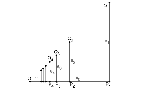
It is not difficult to see that is a complete geodesics space. For with coordinates in , let
Denoting , by direct calculations, for any we have
(Here we choose the optimal integration path from to and then to .) We thus observe that as , but .
Lemma 2.5 (Completeness).
Proof.
Suppose that is a Cauchy sequence with respect to the metric . Thanks to (2.1) in Lemma 2.1, we see that is also a Cauchy sequence with respect to the metric . Since is a closed set in the complete space , there exists such that as .
By definition of Cauchy sequences, for any , we can take such that for all . Similarly, we can choose with satisfying for all . We repeat this process to obtain a sequence such that . By definition of , we can find curves in joining and such that
Concatenating these curves in order, we build a curve connecting to satisfying
which yields . In view of the arbitrariness of , we have actually proved the convergence of to in the metric . ∎
We cannot guarantee the compactness of without imposing further assumptions. Indeed, in Example 2.4 we see that the sequence is bounded but without a convergent subsequence in ; indeed, for each we have that . It follows that is not compact.
3. Monge Solutions and Comparison Principle
3.1. Definition of Monge solutions
Let us now study the Dirichlet problem (1.1), (1.2). We begin with the definition of Monge solutions to (1.1).
Definition 3.1 (Monge solutions).
We say that a locally bounded function is a Monge solution (resp. subsolution, supersolution) to (1.1) in if for every ,
| (3.1) |
We stress that the topology in the local boundedness of and limsup in the definition above is taken with respect to the metric . Since implies by (2.1), we see that
| (3.2) |
implies
| (3.3) |
In general, we cannot expect that the reverse inequality of (3.3) holds without further assumptions like (1.14).
We also emphasize that our definition does not require any continuity or semicontinuity of . This relaxation constitutes a difference from the standard definition of discontinuous viscosity solutions. Recall that when defining a (possibly discontinuous) subsolution , we usually assume (and for the symmetric supersolution definition). Here, and denote the classes of upper and lower semicontinuous functions in respectively with respect to . We do not adopt such restrictions here.
Remark 3.2.
Using the subslope defined in (1.10), we can see in a straightforward manner that our Monge solutions (resp., subsolutions, supersolutions) of (1.1) can simply be understood as Monge solutions (resp., subsolutions, supersolutions) of
| (3.4) |
Proposition 3.3.
On the other hand, Definition 3.1, together with (1.14), does not guarantee the upper semicontinuity of a Monge solution. However, for Monge solutions that arise from the associated Dirichlet problem, we will later use its optimal control interpretation to show the continuity of solutions.
Thanks to the metric change, one can essentially apply the results in [43] to (3.4) in the complete metric space to show both uniqueness and existence of Monge solutions of (1.1)(1.2) under appropriate assumptions on the boundary data . The compatibility condition (1.13) we will impose on , combined with (1.14), basically ensures that the topology stays equivalent when converting the metric from to .
3.2. Comparison principle
Let us prove a comparison principle, where we assume the semicontinuity of Monge sub- and supersolutions with respect to the metric . We say that is upper (resp., lower) semicontinuous with respect to , denoted by (resp., ), if for every fixed , we have
It is not difficult to see that (resp., ) if (resp., ) with respect to , since implies that .
Theorem 3.4 (Comparison principle for Monge solutions).
Proof.
Since and are bounded, we may assume that by adding a positive constant to them. It suffices to show that in for all . Assume by contradiction that there exists such that for some . By (3.5), we may take small such that
for all , where we denote for . We choose small, where is the lower bound of as in (1.3), such that
and
| (3.6) |
Thus there exists such that and therefore .
In view of Lemma 2.5, we see that is complete. Since are bounded from above and upper semicontinuous in with respect to the metric , by Ekeland’s variational principle (cf. [23, Theorem 1.1], [24, Theorem 1]), there exists such that
| (3.7) |
and
| (3.8) |
Note that by (2.1), the relation (3.7) combined with the choice of implies that . Then from (3.8), it follows that
| (3.9) |
when is small enough. Hence, by (2.1) we get
By the Monge subsolution property of and the Monge supersolution property of , it follows that , which is a contradiction to (3.6). Hence, we obtain in for all . Letting , we end up with in . Our proof is thus complete. ∎
Remark 3.5.
If in Theorem 3.4 we further assume that is compact, then the proof becomes simpler. Under this assumption, there is no need to use Ekeland’s variational principle, since is upper semicontinuous and hence attains a maximum at a point in the compact set . The condition (3.5) can also be simplified; it is sufficient to assume that on , since it guarantees a positive maximum of in for in our proof above. We summarize this observation in the following theorem.
Theorem 3.6 (Comparison principle in a compact space).
We would also like to remark that the comparison results may be applied to the situation with only partial boundary data (or the so-called boundary condition in the viscosity sense). In general, even though is prescribed on , a Monge solution may only fulfill the condition on a subset of . We discuss such situation in detail in Section 4.2.
We concluding this section by remarking that the boundedness condition on and in Theorem 3.4 is essential. In fact, without assuming the boundedness, we have the following simple counterexample for uniqueness of Monge solutions.
Example 3.7.
Let be the unit circle in , centered at , that is,
Here is a complete geodesic space with its intrinsic length metric. Let and . Take to be
See Figure 2.
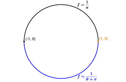
Note that
is a Monge solution of (1.1), (1.2), which can be derived from the formula (1.16) in Theorem 1.1. Note that as , we must have . On the other hand, we observe that
is also a Monge solution that also satisfies (1.17). This example shows that in general we may have multiple solutions, continuous but unbounded in . In this example, once we equip with the metric , the topology on changes so that now is homeomorphic to the Euclidean set , with boundary . In effect, is no longer connected with respect to the topology generated by the metric , allowing us to construct two distinct solutions.
4. Existence of Monge solutions
In this section, we establish an optimal control interpretation of the Dirichlet boundary condition (1.2) for the problem (1.1) and prove our main result, Theorem 1.1. We also discuss the case when the boundary compatibility condition (1.13) fails to hold and turn it into another Dirichlet problem of the same type but with reduced boundary data.
4.1. Optimal control formulation for the Dirichlet problem
Recall that the standing assumption (1.9) still holds. In other words, there exist curves in connecting any such that . It is a condition on as well as the regularity of .
Lemma 4.1 (Lipschitz continuity in ).
Let be a complete length space, be a bounded domain, satisfy (1.3), and be bounded. Then the function , as defined by (1.16), satisfies
| (4.1) |
In particular, is Lipschitz in with respect to and hence locally bounded with respect to the topology generated by . Moreover, if (1.14) holds, then is uniformly continuous in with respect to .
Proof.
Let us now prove our main result, Theorem 1.1.
Proof of Theorem 1.1.
We first show (i). By Lemma 4.1, we see that is Lipschitz with respect to and is a Monge subsolution; indeed, by (4.1) we have that for any ,
| (4.2) |
and thus
| (4.3) |
On the other hand, in view of the definition of from (1.16), for any and any , there exist and such that
| (4.4) |
Let be a point on with and denote by the portion of between and . Then by (1.16) again, we deduce that
It follows that
which, by (1.3), yields
Due to the arbitrariness of and , we obtain the Monge supersolution property of . We have thus shown that is a Monge solution of (1.1) in the sense of Definition 3.1.
Let us show (ii) and (iii). We prove (1.17) under the additional compatibility condition (1.13) on the boundary value . Indeed, fixing and arbitrarily, by the definition of in (1.16) we can see that
| (4.5) |
For any small, the definition of also implies the existence of such that
| (4.6) |
Since the compatibility condition (1.13) yields
applying Lemma 2.1 we deduce from (4.6) that
Combining (4.5) with the above inequality we obtain
| (4.7) |
for all and . Therefore,
| (4.8) | ||||
By the additional assumption (1.15), we obtain (1.17) by passing to the limit of (4.8) as . In particular, we have on . The uniqueness of solutions follow from the comparison principle, Theorem 3.4. Suppose that there is another such solution satisfying (1.17). For any with , we can find such that and
By (1.17), this yields (3.5). Using Theorem 3.4, we end up with in , which completes the proof of (ii).
Remark 4.2.
Following Example 2.3, we now give an explicit example of unique Monge solution of the Dirichlet problem in one dimension with inhomogeneous term.
Example 4.3.
The statement (i) in Theorem 1.1 is a very general existence result for Monge solutions. It allows us to have a discontinuous (with respect to ) Monge solution of (1.1) even when (1.14) fails to hold. In this case, under the assumptions of (ii), we have unique existence of a solution that is Lipschitz with respect to but possibly discontinuous in the metric . Below we give a typical example illustrating such behavior based on Example 2.4.
Example 4.4.
Let and be given as in Example 2.4. Let ; in other words, we set . Also, we take at . We have shown in Example 2.4 that is complete with respect to the metric . Applying Theorem 1.1(ii), we obtain a unique Monge solution of (1.1)(1.2) satisfying (1.17). In particular, by (1.16) we have , for all . This clearly shows that is not continuous at with respect to the metric . However, is Lipschitz continuous with respect to the metric .
Let us present an additional property of the Monge solution , which is a direct generalization of [43, Proposition 4.15].
Proposition 4.5 (Additional regularity).
4.2. Loss of boundary data and reduced Dirichlet problem
In general, the condition (1.13) may not hold. As a result, it is possible that holds only on a subset of . This set may also depend on but we write to emphasize that it is the part where the Dirichlet condition is maintained. The loss of boundary data occurs on . At points the Monge condition (3.1) holds, and so the function constructed in (1.16) solves the problem in the new domain . We thus can use the comparison results above with replaced by to guarantee the uniqueness of solutions. The following typical, well-understood example in reveals such a situation.
Example 4.6.
Let and in . Set and . It turns out that there are no solutions that are continuous in and satisfy both (1.1) and (1.2) simultaneously. However, is the unique solution that satisfies only the partial boundary condition . In fact, holds and we can still use the comparison principle if we consider and . One can certainly take another solution for , which is a Monge solution in and satisfies the boundary condition . However, this solution does not satisfy the Monge condition (3.1) at , and moreover, such solutions are not necessarily unique from the PDE viewpoint; is also a Monge solution in with . Indeed, it is the only Monge solution in with boundary data . We resolve the uniqueness issue by taking so that is the only solution in satisfying . The function is regarded as a natural choice of the unique solution here also due to the optimal control interpretation given by (1.16).
Let us provide a more general result for the case when (1.13) fails to hold and on . As explained at the end of Section 3, we still expect that there exists a solution such that on a subset of . In fact, we take
| (4.11) |
By (1.16), it is clear that
| (4.12) |
In general, the set may be empty. However, if is compact with respect to and and , or if is compact with respect to and . In either case, contains the minimizers of on . Also, is a closed set with respect to the metric .
Using we can reduce the original Dirichlet problem to
| (4.13) |
with boundary condition
| (4.14) |
It turns out that given by (1.16) is the unique Monge solution of (4.13), (4.14) when . Here, for these new Monge solutions, we certainly need to extend the definition of Monge solutions to . More precisely, we say a locally bounded function is a Monge solution of (4.13) if it satisfies the property in Definition 3.1 with playing the role of the domain there, and with (3.1) replaced by
| (4.15) |
One can define Monge subsolutions and supersolutions of (4.13) in a similar way.
Proposition 4.7 (Well-posedness with possible loss of boundary data).
Let be a complete length space and be a bounded domain. Assume that (1.3) and (1.9) hold. Let be bounded and be defined by (1.16). Let be given by (4.11). Then is a Monge solution of (4.13), (4.14). If in addition and (1.15) holds, then is the unique Lipschitz (with respect to ) Monge solution of the Dirichlet problem (4.13)(4.14) satisfying
| (4.16) |
Proof.
We have shown in Theorem 1.1 that is a Monge solution in . Part of the proof holds also for boundary points. In fact, by (4.1) we get, for any fixed ,
which yields (4.3) with . Now, for any , since , by (1.16), for any we still have (4.4) for some and . Then we can follow the same argument in the proof of Theorem 1.1 to prove that
Hence, (4.15) holds for all . In view of (4.12), we also have on . Thus is a Monge solution of (4.13), (4.14).
Remark 4.8.
In the Euclidean space, when and , we usually relax the meaning of the Dirichlet condition on , requiring to satisfy
| (4.17) |
in the viscosity sense. Under appropriate assumptions on the regularity of , one can show that the generalized Dirichlet (or state constraint) problem still admits a unique viscosity solution [51, 52, 37]. Our result in Proposition 4.7 essentially handles this type of generalized Dirichlet boundary problems in metric spaces. In fact, we have (4.15) at each , which corresponds to the viscosity inequality (4.17). Such topological change was also observed in [42, Remark 5.10] for evolutionary Hamilton-Jacobi equations in metric spaces.
5. Existence of admissible curves and regularity of solutions
We have seen that the existence of admissible curves (1.9) plays an important role in finding the Monge solutions of (1.1). The consistency of local topology condition (1.14), which guarantees the continuity with respect to the original metric and uniqueness of the Monge solution of the Dirichlet problem, is also related to the existence of admissible curves. We already provided an example, Example 2.4, to show that (1.14) fails to hold in general. It is natural to ask under what assumptions we can obtain (1.9) and (1.14). In this section, we attempt to answer this question.
We introduce some notations and definitions for our use in this section. Let be a metric measure space with being a locally finite Borel measure. We use to denote an open ball when the center and radius are irrelevant to our analysis. In this case, we also write for any for simplicity of notation.
Let . Let be a collection of nonconstant rectifiable curves in . We say that a curve connecting is a -quasiconvex curve if the length of the curve is at most . Let denote the collection of -quasiconvex curves connecting . A metric space is said to be quasiconvex if there exists such that every pair of points can be connected by a -quasiconvex curve.
Let be the family of all Borel measurable functions such that for every . For each , the -modulus of is defined as
and the -modulus of is defined as
For any given function , a Borel function is said to be a -weak upper gradient of if
holds for all rectifiable paths outside a family of curves with -modulus zero. Consult [30] for an introduction about modulus of curve family and upper gradients.
Let . A metric measure space is said to support a -Poincaré inequality if there exist constants and such that for every measurable function and every upper gradient of , the pair satisfies
| (5.1) |
on every ball . If , the right hand side above is replaced by Here and in the sequel, for an integrable function and a measurable set of finite measure, we take
We say that a metric measure space is a PI-space if the measure is doubling and the space supports a -Poincaré inequality for some .
Theorem 5.1 (Regularity in -PI spaces).
Let be a complete doubling metric measure space supporting a -Poincaré inequality with , where is the homogeneous dimension satisfying (1.18). Then there exists a constant depending on the constants of PI-space and such that for every function and its -weak upper gradient , the following inequality holds for each open ball and every :
| (5.2) |
where is the scaling constant in Poincaré inequality. Furthermore, for any pair of distinct points , there exists depending on the constants of PI-space and such that
| (5.3) |
where is the family of all rectifiable curves in joining and .
A stronger version of the above result on Ahlfors -regular space with can be found in [21, Theorem 5.1].
Proof of Theorem 5.1.
The proof of (5.2) can be found in [30, Theorem 9.2.14]. We only show the modulus estimate (5.3) below. We only consider a pair of distinct points such that . Otherwise, the proof is complete. We pick , that is, for every rectifiable curve . Define
and then is measurable [39, Corollary 1.10] and is an upper gradient of . In fact, it is clear that and
Therefore is an upper gradient for in . It follows that is also an upper gradient for .
Let be a Lipschitz function satisfying that , on and on . Define a function . It easily follows that and . One can also verify that is an upper gradient of . In particular, since on , we obtain is an upper gradient for on . Hence, it follows that
Since is arbitrary, by definition we obtain (5.3). ∎
This theorem implies the following result.
Proposition 5.2 (Hölder regularity).
Proof.
In general, if for , then (1.9) may not hold in general, as can be seen in the following simple example, which is an adaptation of Example 2.3.
Example 5.3.
Let with being the Euclidean metric and being the one-dimensional Lebesgue measure. Let and
It is clear that for any . Then for any , and .
The critical case is complicated. For with , we can prove the conditions (1.9) and (1.14) if , since the -modulus of the curve collection containing just one non-constant curve is positive. In general, we cannot expect the results in Proposition 5.2 to always hold if but for any . On the other hand, (1.9) is only about the existence of one curve on which is integrable and can be obtained even for some functions . A simple example is as below.
Example 5.4.
Let and with denoting the origin . That is, is the unit disk in centered at . We set
Let be given by
Observe that for but ; the value of on does not affect the integral of in . However, for each pair of distinct points , one can find a curve in . For , we can take a curve connecting first to along the circular arc and then to along the horizontal line segment. This choice enables us to guarantee , which shows that a bounded metric space with respect to the metric . The topology induced by , however, is distinct from the Euclidean topology. Indeed, for and any curve joining and , denoting by the portion of in the Euclidean disk , we have , which yields for all . Hence, as , although converges to in the Euclidean topology. (As the metric is locally bi-Lipschitz equivalent to the Euclidean metric in as well, we see that this sequence cannot converge in with respect to .)
The following result, which can be found in [21, Theorem 3.1] and [22, Theorem 2.10], is a variant of Theorem 5.1 for the case .
Theorem 5.5 (Regularity in -PI spaces).
Let be a complete doubling metric measure space. Then the following statements are equivalent.
-
(1)
supports an -Poincaré inequality.
-
(2)
There exists such that for all satisfying , where we recall that denotes the collection of -quasiconvex curves connecting .
-
(3)
There exists such that whenever with and with , there is a quasiconvex curve joining such that and , where denotes the one-dimensional Hausdorff measure.
The following is the version of Proposition 5.2 corresponding to .
Proposition 5.6 (Lipschitz regularity).
Proof.
It is not difficult to see that Theorem 5.5 (2) implies (1.9). The proof of (1.14) involves the condition (3) in Theorem 5.5. In fact, since , there exist a null set such that
| (5.6) |
Then by Theorem 5.5, for any , we can take a curve in joining them with and , which yields (5.5). Thus (1.14) clearly holds. ∎
Since the Monge solution defined by (1.16) is Lipschitz in the metric , as shown in Theorem 1.1, we obtain Theorem 1.2 as an immediate consequence of Proposition 5.2 and Proposition 5.6. Under the same assumptions, it is not difficult to show that is in the Sobolev class , that is, and has an upper gradient in . In fact, by (1.8) and (4.1) we see that is an upper gradient of .
6. Solutions for admissible curves transversal to null sets
In this section, we assume that satisfies (1.3) and is a complete doubling metric measure space with homogeneous dimention . Assuming either of the additional regularity assumptions (A1) and (A2) as stated in the discussion following (1.18), we consider a slightly different optical length function and the associated solutions using curves transversal to null sets in . This change improves the stability of solutions with respect to the perturbation on . We refer to [46, 44] for stability results on time-dependent Hamilton-Jacobi equations in metric spaces.
6.1. Optical length with transversal curves
Let be the collection of arc-length parametrized rectifiable curves in connecting with and transversal to a given null set , as given in (1.19). The associated optical length function is defined by (1.20).
Under the standing assumptions of this section, we consider if (A1) holds. Note that with . Proposition 5.2 then implies that if , and we can verify that and
If (A2) holds, then Theorem 5.5 implies that and therefore for any distinct points . Hence, in either case we have
| (6.1) |
We define the maximal optical length function by (1.22). It is easy to verify using Proposition 5.6 and Proposition 5.2 that the optical length function (as well as for any fixed null set ) also satisfies the metric properties, as discussed for in Lemma 2.1.
Moreover, we see that (1.14) holds for under either of the assumptions (A1), (A2). Indeed, it is an immediate consequence of Proposition 5.2 when (A1) holds. In the case of (A2), there exists a null set such that (5.6) holds. Since supports an -Poincaré inequality, by Theorem 5.5, there exists such that for any null set and we can find a curve transversal to satisfying
Recall that . It follows that
| (6.2) |
and thus (1.14) holds for . Furthermore, under the assumption (1.3), together with (2.1), we also obtain
| (6.3) |
Since for each null set , it is easily seen that
| (6.4) |
It turns out that the supremum in the definition of can be attained at a particular null set if either (A1) or (A2) holds.
Lemma 6.1.
Let be a complete metric measure space with a doubling measure. If (A1) or (A2) holds, then there exists a null set such that defined in (1.22) satisfies
| (6.5) |
Proof.
It suffices to show , since the reverse inequality holds obviously. We first fix a null set , and we now show that for any fixed there exists a null set containing such that
To see this, for any , we take a null set () such that
Set . Then,
and thus by letting . The claim is proved.
Since is complete and doubling, it follows that is separable [30, Lemma 4.1.13], and therefore there exists a countable dense subset . For every pair of points , there exists a null set containing such that
We construct a null set in slightly different ways for the cases (A1) and (A2).
If (A1) holds, we set . Then we have and
| (6.6) |
Fix and arbitrarily. Set with constant from (5.4) and let and . Proposition 5.2 implies that
| (6.7) |
There exists a null set containing such that
| (6.8) |
For , we can apply Theorem 5.1 to find a curve transversal to connecting and . In particular, there exists a curve such that
| (6.9) |
Analogously, there exists a curve transversal to a null set containing and connecting in such that
| (6.10) |
Choose any curve and let be a curve connecting and defined by joining , and . Therefore we obtain
| (6.11) | ||||
Since is arbitratry, it follows that
for all . We have completed the proof of (6.5) under the assumption (A1).
If, on the other hand, (A2) holds, then there exists a null set such that (5.6) holds. We define in this case. It is clear that is still a null set. For every , let . Then for any and and , there exists a null set containing such that (6.8) holds also in this case. Thanks to the -Poincaré inequality, we adopt (5.5) in Proposition 5.6 to get (6.7). The rest of the proof is the same as that under the assumption (A1). We find curves and satisfying estimates (6.9) and (6.10), and build again by concatenating and . The same estimate as in (6.11) yields (6.5) in this case. ∎
6.2. Transversal Monge solutions
Using the optical length (or equivalently with given in Lemma 6.1), we can consider a different notion of Monge solutions, which we call transversal Monge solutions.
Definition 6.2 (Transversal Monge solutions).
We say that a locally bounded function is a transversal Monge solution (resp. subsolution, supersolution) to (1.1) in if for any
| (6.12) |
Remark 6.3.
Remark 6.4.
Following Remark 3.2, we can show that holds for any transversal Monge solution and any where is continuous.
We can repeat our arguments in the previous section, replacing by , to prove the uniqueness and existence of transversal Monge solutions of (1.1)(1.2). Note that thanks to (A1) or (A2), is bounded if is bounded. Below we give the statements without proofs.
Theorem 6.5.
Theorem 6.6.
Let be a complete geodesic space with doubling and let be a bounded domain. Assume that satisfies (1.3) and that either (A1) or (A2) holds. Let be bounded, and let be defined by (1.21), where is given by (1.22). Then is a transversal Monge solution of (1.1), which is Lipschitz continuous with respect to and uniformly continuous with respect to in . Moreover, if satisfies
| (6.14) |
then is the unique transversal Monge solution of (1.1)(1.2).
Remark 6.7.
Recall that a metric space is said to be proper if every closed and bounded set is compact. A complete metric measure space with doubling is proper [30, Lemma 4.1.14]. Furthermore, Hopf-Rinow Theorem implies that a complete and proper length space is a geodesic space.
The Lipschitz continuity of can be obtained via the relation
| (6.15) |
which is a counterpart of (4.1) in the current setting.
6.3. Maximal weak solutions
In the Euclidean space, for bounded continuous inhomogeneous term , one can define weak solutions of (1.1) by requiring the function to be locally Lipschitz and satisfies the equation almost everywhere in . Such kind of solutions are also called Lipschitz a.e. solutions in the literature. We extend this notion to metric measure spaces for a possibly discontinuous .
Definition 6.8.
We say that is a weak solution (resp. subsolution, supersolution) to (1.1) if the slope exists and satisfies (resp. , ) at almost every .
When the measure on is doubling and supports an -Poincaré inequality, we know from [20] that is Lipschitz continuous with respect to the metric and that is the least -weak upper gradient of . Our construction of in this setting yields and in general we may not have equality. However, if is continuous almost everywhere, we do obtain that . This is the focus of this subsection.
We can show that the maximal weak subsolution is the transversal Monge solution provided that is upper semicontinuous almost everywhere and the metric space satisfies the -weak Fubini property. A metric measure space is said to satisfy the -weak Fubini property if for any null set and , given any distinct points , there exists a curve connecting transversal to such that . In particular, a space satisfying the -weak Fubini necessarily supports an -Poincaré inequality. More discussion on the -weak Fubini property can be found in [22, Section 4].
Proposition 6.9.
Let be a complete geodesic space with a doubling measure. Suppose that is a bounded domain with satisfying the -weak Fubini property. Assume that and that satisfies (1.3). Let satisfy (6.14) and be the transversal Monge solution defined in (1.21). Then, in holds for all . If in addition is assumed to be upper semicontinuous almost everywhere, i.e., there exists a set with such that is upper semicontinuous, then is a weak subsolution of (1.1), (1.2). In particular, is the maximal weak subsolution in the sense that
| (6.17) |
Remark 6.10.
If we further assume that supports a -Poincaré inequality for some , then we have almost everywhere [15, Theorem 6.1], where denotes the least -weak upper gradient of . In particular, the function defined in (1.16) is the maximal Lipschitz solution to the Dirichlet problem
where satisfy the conditions in Proposition 6.9.
Proof of Proposition 6.9.
We have seen in Theorem 6.6 that is uniformly continuous in with respect to the metric . Let us show that in for every . Take the null set . Note that is an upper gradient of , i.e.,
holds for every curve joining and in ; see [30, Lemma 6.2.6]. Let , where is the null set given in Lemma 6.1. It is clear that is still a null set. We fix . For any , we can choose a curve in connecting and such that it is transversal to and
| (6.18) |
This is possible because supports the -weak Fubini property. Due to the transversality, we get
Hence, it follows that
By (6.18), we thus have . Since is arbitrary, it follows that for every .
We next prove that is a weak solution of (1.1) under the upper semicontinuity of for a null set . Let and fix arbitrarily. In view of Remark 6.4, satisfies . In what follows we show that . Then by the upper semicontinuity of , for every we can take small such that
| (6.19) |
Using the -weak Fubini property of , for any it is possible to connect and by a curve in that is transversal to and satisfies . This implies that for any ; in other words, lies in . It follows from (6.19) and the transversality of to that
Applying (6.5) in Lemma 6.1, we therefore obtain
for all with small.
In view of the Lipschitz continuity of in (6.15), we get
Dividing the inequality by , letting and then sending , we end up with . Since is arbitrary and is a null set, we see that is a weak subsolution of (1.1). Note that holds on thanks to the definition (1.21). Hence, . Combining this with the first part of our result, we are led to (6.17). ∎
Remark 6.11.
We can define the class of weak supersolution and solution by replacing “" in (6.16) by and respectively. If is further assumed to be continuous, then by Remark 6.4, satisfies for any . It immediately follows that due to the property . In other words, is a weak supersolution of (1.1) since follows from (6.14). Since is also a weak subsolution, we see that is a weak solution.
References
- [1] Y. Achdou, F. Camilli, A. Cutrì, and N. Tchou. Hamilton-Jacobi equations constrained on networks. NoDEA Nonlinear Differential Equations Appl., 20(3):413–445, 2013.
- [2] P. Albano. On the eikonal equation for degenerate elliptic operators. Proc. Amer. Math. Soc., 140(5):1739–1747, 2012.
- [3] P. Albano, P. Cannarsa, and T. Scarinci. Regularity results for the minimum time function with Hörmander vector fields. J. Differential Equations, 264(5):3312–3335, 2018.
- [4] L. Ambrosio and J. Feng. On a class of first order Hamilton-Jacobi equations in metric spaces. J. Differential Equations, 256(7):2194–2245, 2014.
- [5] L. Ambrosio, N. Gigli, and G. Savaré. Heat flow and calculus on metric measure spaces with Ricci curvature bounded below—the compact case. In Analysis and numerics of partial differential equations, volume 4 of Springer INdAM Ser., pages 63–115. Springer, Milan, 2013.
- [6] M. Bardi and I. Capuzzo-Dolcetta. Optimal control and viscosity solutions of Hamilton-Jacobi-Bellman equations. Systems & Control: Foundations & Applications. Birkhäuser Boston Inc., Boston, MA, 1997. With appendices by Maurizio Falcone and Pierpaolo Soravia.
- [7] T. Bieske. The Carnot-Carathéodory distance vis-à-vis the eikonal equation and the infinite Laplacian. Bull. Lond. Math. Soc., 42(3):395–404, 2010.
- [8] A. Briani and A. Davini. Monge solutions for discontinuous Hamiltonians. ESAIM Control Optim. Calc. Var., 11(2):229–251 (electronic), 2005.
- [9] D. Y. Burago. Periodic metrics. In Representation theory and dynamical systems, volume 9 of Adv. Soviet Math., pages 205–210. Amer. Math. Soc., Providence, RI, 1992.
- [10] L. Caffarelli, M. G. Crandall, M. Kocan, and A. Swi\polhk ech. On viscosity solutions of fully nonlinear equations with measurable ingredients. Comm. Pure Appl. Math., 49(4):365–397, 1996.
- [11] F. Camilli. An Hopf-Lax formula for a class of measurable Hamilton-Jacobi equations. Nonlinear Anal., 57(2):265–286, 2004.
- [12] F. Camilli and A. Siconolfi. Hamilton-Jacobi equations with measurable dependence on the state variable. Adv. Differential Equations, 8(6):733–768, 2003.
- [13] F. Camilli and A. Siconolfi. Time-dependent measurable Hamilton-Jacobi equations. Comm. Partial Differential Equations, 30(4-6):813–847, 2005.
- [14] P. Cardaliaguet. Notes on mean field games (from P.-L. Lions’ lectures at collége de france). https://www.ceremade.dauphine.fr/ cardaliaguet/MFG20130420.pdf, 2013.
- [15] J. Cheeger. Differentiability of Lipschitz functions on metric measure spaces. Geom. Funct. Anal., 9(3):428–517, 1999.
- [16] Q. Chen, S. A. R. Horsley, N. J. G. Fonseca, T. Tyc, and O. Quevedo-Teruel. Double-layer geodesic and gradient-index lenses. Nature Communications, 13(1):2354, 2022.
- [17] X. Chen and B. Hu. Viscosity solutions of discontinuous Hamilton-Jacobi equations. Interfaces Free Bound., 10(3):339–359, 2008.
- [18] M. G. Crandall, M. Kocan, P. L. Lions, and A. Świ\polhkech. Existence results for boundary problems for uniformly elliptic and parabolic fully nonlinear equations. Electron. J. Differential Equations, pages No. 24, 22 pp. 1999.
- [19] K. Deckelnick and C. M. Elliott. Uniqueness and error analysis for Hamilton-Jacobi equations with discontinuities. Interfaces Free Bound., 6(3):329–349, 2004.
- [20] E. Durand-Cartagena and J. A. Jaramillo. Pointwise Lipschitz functions on metric spaces. J. Math. Anal. Appl., 363(2):525–548, 2010.
- [21] E. Durand-Cartagena, J. A. Jaramillo, and N. Shanmugalingam. Geometric characterizations of -Poincaré inequalities in the metric setting. Publ. Mat., 60(1):81–111, 2016.
- [22] E. Durand-Cartagena, J. A. Jaramillo, and N. Shanmugalingam. Existence and uniqueness of -harmonic functions under assumption of -Poincaré inequality. Math. Ann., 374(1-2):881–906, 2019.
- [23] I. Ekeland. On the variational principle. J. Math. Anal. Appl., 47:324–353, 1974.
- [24] I. Ekeland. Nonconvex minimization problems. Bull. Amer. Math. Soc. (N.S.), 1(3):443–474, 1979.
- [25] F. Essebei, G. Giovannardi, and S. Verzellesi. Monge solutions for discontinuous Hamilton-Jacobi equations in Carnot groups, preprint, 2023.
- [26] W. Gangbo and A. Świ\polhkech. Metric viscosity solutions of Hamilton-Jacobi equations depending on local slopes. Calc. Var. Partial Differential Equations, 54(1):1183–1218, 2015.
- [27] Y. Giga, P. Górka, and P. Rybka. A comparison principle for Hamilton-Jacobi equations with discontinuous Hamiltonians. Proc. Amer. Math. Soc., 139(5):1777–1785, 2011.
- [28] Y. Giga and N. Hamamuki. Hamilton-Jacobi equations with discontinuous source terms. Comm. Partial Differential Equations, 38(2):199–243, 2013.
- [29] Y. Giga, N. Hamamuki, and A. Nakayasu. Eikonal equations in metric spaces. Trans. Amer. Math. Soc., 367(1):49–66, 2015.
- [30] J. Heinonen, P. Koskela, N. Shanmugalingam, and J. T. Tyson. Sobolev spaces on metric measure spaces, volume 27 of New Mathematical Monographs. Cambridge University Press, Cambridge, 2015. An approach based on upper gradients.
- [31] J. Hong, W. Cheng, S. Hu, and K. Zhao. Representation formulas for contact type Hamilton-Jacobi equations. J. Dynam. Differential Equations, 34(3):2315–2327, 2022.
- [32] R. A. Houstoun. Note on Einstein’s theory of gravitation. Philos. Mag. (7), 33:899–903, 1942.
- [33] C. Imbert and R. Monneau. Flux-limited solutions for quasi-convex Hamilton-Jacobi equations on networks. Ann. Sci. Éc. Norm. Supér. (4), 50(2):357–448, 2017.
- [34] C. Imbert and R. Monneau. Quasi-convex Hamilton-Jacobi equations posed on junctions: The multi-dimensional case. Discrete Contin. Dyn. Syst., 37(12):6405–6435, 2017.
- [35] C. Imbert, R. Monneau, and H. Zidani. A Hamilton-Jacobi approach to junction problems and application to traffic flows. ESAIM Control Optim. Calc. Var., 19(1):129–166, 2013.
- [36] H. Ishii. Hamilton-Jacobi equations with discontinuous Hamiltonians on arbitrary open sets. Bull. Fac. Sci. Engrg. Chuo Univ., 28:33–77, 1985.
- [37] H. Ishii. A boundary value problem of the Dirichlet type for Hamilton-Jacobi equations. Ann. Scuola Norm. Sup. Pisa Cl. Sci. (4), 16(1):105–135, 1989.
- [38] H. Ishii and H. Mitake. Representation formulas for solutions of Hamilton-Jacobi equations with convex Hamiltonians. Indiana Univ. Math. J., 56(5):2159–2183, 2007.
- [39] E. Järvenpää, M. Järvenpää, K. Rogovin, S. Rogovin, and N. Shanmugalingam. Measurability of equivalence classes and -property in metric spaces. Rev. Mat. Iberoam., 23(3):811–830, 2007.
- [40] P.-L. Lions. Generalized solutions of Hamilton-Jacobi equations, volume 69 of Research Notes in Mathematics. Pitman (Advanced Publishing Program), Boston, Mass.-London, 1982.
- [41] Q. Liu and A. Mitsuishi. Principal eigenvalue problem for infinity Laplacian in metric spaces. Adv. Nonlinear Stud., 22(1):548–573, 2022.
- [42] Q. Liu and A. Nakayasu. Convexity preserving properties for Hamilton-Jacobi equations in geodesic spaces. Discrete Contin. Dyn. Syst., 39(1):157–183, 2019.
- [43] Q. Liu, N. Shanmugalingam, and X. Zhou. Equivalence of solutions of eikonal equation in metric spaces. J. Differential Equations, 272:979–1014, 2021.
- [44] S. Makida. Stability of viscosity solutions on expanding networks. preprint, 2023.
- [45] A. Nakayasu. Metric viscosity solutions for Hamilton-Jacobi equations of evolution type. Adv. Math. Sci. Appl., 24(2):333–351, 2014.
- [46] A. Nakayasu and T. Namba. Stability properties and large time behavior of viscosity solutions of Hamilton-Jacobi equations on metric spaces. Nonlinearity, 31(11):5147–5161, 2018.
- [47] R. T. Newcomb, II and J. Su. Eikonal equations with discontinuities. Differential Integral Equations, 8(8):1947–1960, 1995.
- [48] D. N. Ostrov. Extending viscosity solutions to eikonal equations with discontinuous spatial dependence. Nonlinear Anal., 42(4, Ser. A: Theory Methods):709–736, 2000.
- [49] D. Schieborn and F. Camilli. Viscosity solutions of Eikonal equations on topological networks. Calc. Var. Partial Differential Equations, 46(3-4):671–686, 2013.
- [50] B. D. Seckler and J. B. Keller. Geometrical theory of diffraction in inhomogeneous media. J. Acoust. Soc. Amer., 31:192–205, 1959.
- [51] H. M. Soner. Optimal control with state-space constraint. I. SIAM J. Control Optim., 24(3):552–561, 1986.
- [52] H. M. Soner. Optimal control with state-space constraint. II. SIAM J. Control Optim., 24(6):1110–1122, 1986.
- [53] P. Soravia. Boundary value problems for Hamilton-Jacobi equations with discontinuous Lagrangian. Indiana Univ. Math. J., 51(2):451–477, 2002.
- [54] P. Soravia. Degenerate eikonal equations with discontinuous refraction index. ESAIM Control Optim. Calc. Var., 12(2):216–230, 2006.
- [55] A. Tourin. A comparison theorem for a piecewise Lipschitz continuous Hamiltonian and application to shape-from-shading problems. Numer. Math., 62(1):75–85, 1992.
- [56] H. V. Tran and Y. Yu. Optimal convergence rate for periodic homogenization of convex Hamilton-Jacobi equations, 2022.
- [57] C. Villani. Optimal transport, volume 338 of Grundlehren der Mathematischen Wissenschaften [Fundamental Principles of Mathematical Sciences]. Springer-Verlag, Berlin, 2009. Old and new.