∎
email:chenmh@lzu.edu.cn;
Discovery of subdiffusion problem with noisy data via deep learning
Abstract
Data-driven discovery of partial differential equations (PDEs) from observed data in machine learning has been developed by embedding the discovery problem. Recently, the discovery of traditional ODEs dynamics using linear multistep methods in deep learning have been discussed in [Racheal and Du, SIAM J. Numer. Anal. 59 (2021) 429-455; Du et al. arXiv:2103.11488]. We extend this framework to the data-driven discovery of the time-fractional PDEs, which can effectively characterize the ubiquitous power-law phenomena. In this paper, identifying source function of subdiffusion with noisy data using approximation in deep neural network is presented. In particular, two types of networks for improving the generalization of the subdiffusion problem are designed with noisy data. The numerical experiments are given to illustrate the availability using deep learning. To the best of our knowledge, this is the first topic on the discovery of subdiffusion in deep learning with noisy data.
Keywords:
Deep learning, discovery of subdiffusion, noisy data1 Introduction
Deep learning has been extended to many different practical fields, including image analysis, natural language processing, system recognizing etc IYA:2016 . There are already some important progress for numerically solving the ODEs and PDEs systems in deep learning. For example, variational methods WEBY:2017 ; YGMK:2021 ; YLJ:2021 ; CGD:2021 , Galerkin methods DGM:2018 ; CJR:2021 , random particle method XUY:2020 , different operators method LZY:2021 , linear multistep method DUQ:2021 . Based on the the neural networks, the data-driven discovery of differential equations has been proposed in RTP:2019 ; SHR:2019 ; DEM:2020 ; MRI:2018 ; QWX:2019 ; DUQ:2021 including the space-fractional differential equations GRPK:19 . In particular, the discovery of traditional ODEs dynamics using linear multistep methods in deep learning have been discussed in DUQ:2021 ; RD:21 and RTP:2019 . Identifying source function from observed data is a meaningful and challenge topic for the time-dependent PDEs.
Over the few decades, fractional models have been attracted wide interest since it can effectively characterize the ubiquitous power-law phenomena with noise data EK:11 ; LWD:17 , which are applied in underground environment problems, transport in turbulent plasma, bacterial motion transport, etc. M2000 . In this work, we study the discovery of the following subdiffusion in deep learning with noise data, whose prototype is LWD:17 ; MS:12 ; WCDBD:22 , for
| (1.1) |
with a positive definite, selfadjoint, linear Laplacian operator. The Caputo fractional derivative Podlubny:99 is defined by
| (1.2) |
and is a given forcing term with noise data. In practice, is not completely known and is disturbed around some known quantity , i.e.,
Here is deterministic and is usually known while no exact behavior exists of the perturbation (noise) term. The uncertainty (lack of information) about (the perturbation term) is naturally represented as a stochastic quantity, see ZK:17 . In the following, we focus on the uniform noise and Gaussian noise. More general noise ZK:17 such as white noise, Wiener process or Brownian motion (which corresponds to the stochastic fractional PDEs LWD:17 ; WCDBD:22 ) can be similarly studied, since it can be discretized as like uniform noise form by a simple arithmetic operations LWD:17 ; MS:12 ; WCDBD:22 .
The main contribution of this paper is to discover subdiffusion via approximation in deep learning with noisy data, where we design two types neural networks to deal with the fractional order , since is a variable parameter. More concretely, we use two strategies (fixed and variable , respectively) to train network, which improves the generalization for the subdiffusion problem. The advantage of first Type is that model (4.2) can be trained for each fixed , which reduces the computational count and required storage, since it fixes as input data. Obviously, it may loss some accuracy. To recover the accuracy, second Type is complemented, which needs more computational count. It implies an interesting generalized structure by combining Type 1 and Type 2, which may keep suitable accuracy and reduces computational count.
The paper is organized as follows. In the next section, we introduce the discretization schemes for the subdiffusion problem (1.1) and its discovery of subdiffusion in Section 3. We construct the discovery of subdiffusion based on the basic deep neural network (DNN) in Section 4. The two types DNN are designed/developed for the subdiffusion model in Section 5. To show the effectiveness of the presented schemes, results of numerical experiments with noisy data are reported in Section 6. Finally, we conclude the paper with some remarks on the presented results.
2 Subdiffusion problem
In this section, we introduce the approximation for solving the subdiffusion. Let , be a partition of the time interval with the grid size . Denote the mesh points , with the uniform grid size , .
The objective for solving the initial value problem in (1.1) is to find the approximation for given source function .
The diffusion term is approximated by a standard second-order discretization:
| (2.1) |
There are serval ways to discretize the Caputo fractional substantial derivative (1.2). For convenience, we use the following standard scheme ChJB:21 ; SOG:17 ; Lin:07 with the truncation error , namely,
| (2.2) |
Here the coefficients are computed by , and
Thus, we approximate (1.1) by the discrete problem with given
| (2.3) |
Remark 2.1
When , the time Caputo fractional derivative uses the information of the classical derivatives at all previous time levels (non-Markovian process). If , it can be seen that by taking the limit in (1.2), which gives the following equation
3 Discovery of subdiffusion
The discovery of subdiffusion is essentially an inverse process of solving a subdiffusion problem (1.2). That means, suppose that only the information of at the pairs of the uniform grid points is provided, we need to recover the source function RD:21 . Assume and both are unknown in subfiffuion system (1.1) with given , the target is to approximate the close-form expression for . We can use the approximated source function to rebuild the discrete relation between and , namely,
| (3.1) |
4 Neural Network approximation
In this section, we introduce the basic deep neural network (DNN) CWHZ:21 ; ZuowShen:2021 ; CGD:2021 ; SHR:2019 , which will be used in discovery of subdiffusion.
4.1 Structure of deep neural network
As the input vector , the neural network can be denoted as
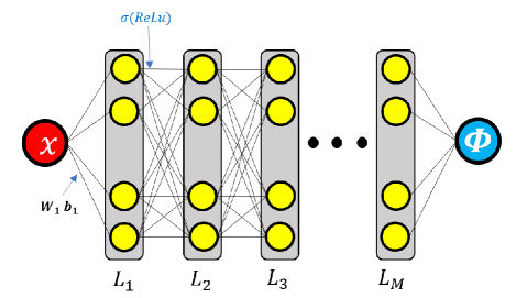
where is a nonlinear function in the whole neural network. The integer is number of the layer of DNN. The -th hidden layer has the following affine transform:
| (4.1) |
where belongs to a parameter functional space . The weight family and collection of bias . The dimensional is the number of neurons (width of neural network) in the m-th layer. The activation function is used as non-linear processing of information. Here we choose the ReLU function as the activation function. All DNN structures can be presented in Figure 1.
4.2 Discovery of subdiffusion in deep learning
Among many different structures of approximations, it is more predominant to employ neural networks as a nonlinear approximation tool to get source function , which is convenient to compute and implement. So the neural network approximation is focused in this paper. Consider the neural network approximation via discertization. We use as the set of all neural networks with special architecture RD:21 . Now we introduce a network to approximate . The model of neural network approximation is developed by replacing each with in (3.1)
| (4.2) |
Now we seek by minimizing the residual error (4.2) under a machine learning framework in practice, namely,
| (4.3) |
with the loss function
| (4.4) |
5 Two types of deep neural networks
It is an interesting question how we can train the discovery of subdiffusion with fractional order , since is variable parameter. Developed the structure of deep neural network in Subsection 4.1, we use two types (fixed and variable , respectively) of DNN for training the discovery of subdiffusion (4.2) in this work.
5.1 Type 1 of DNN: fixed
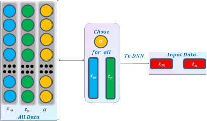
To train the source function of subdiffusion model (4.2) by the deep neural network approximation, we design the Type 1 of DNN for the fixed , see Fig 2, which just needs as input data.
5.2 Type 2 of DNN: variable
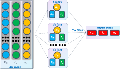
To discover/recover the source function of subdiffusion model (4.2) in DNN, we also design the Type 2 of DNN for the variable , see Fig 3, which uses as input data. Here can be chosen a sequence .
Remark 5.1
The advantage of Type 1 is that model (4.2) can be trained for each fixed , which reduces the computational count and required storage, since it fixes as input data. Obviously, it may loss some accuracy. To recover the accuracy, Type 2 is complemented, which needs more computational count. Hence, there is an interesting generalized structure by combining Type 1 and Type 2, which keeps suitable accuracy and reduces computational count.
6 Numerical Experiments
In this section, we discover subdiffusion problem (1.1) with uniform noise and Gaussian noise in deep learning. More general noise ZK:17 such as white noise, Wiener process or Brownian motion (which corresponds to the stochastic fractional PDEs LWD:17 ; WCDBD:22 ) can be similarly studied, since it can be discretized as like uniform noise form by a simple arithmetic operations LWD:17 ; MS:12 ; WCDBD:22 . Several examples are provided to show the performance of subdiffusion discovery via approximation in DNN by Algorithm 1.
| Feature | Statement | |||
|---|---|---|---|---|
| Environment |
|
|||
|
|
|||
|
|
|||
|
|
|||
|
|
The relative error is measured by
| (6.1) |
where we actually use the well-known Frobenius norm of the matrix , i.e.,
6.1 Numerical Experiments for discovery with uniform noise
Example 1
6.1.1 Type 1 in DNN
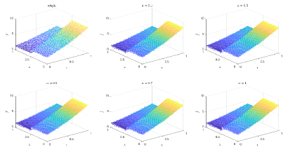
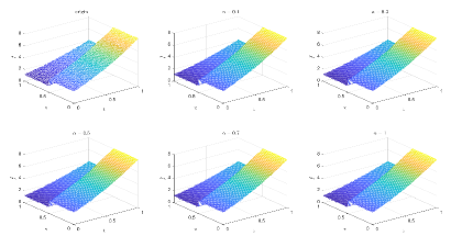
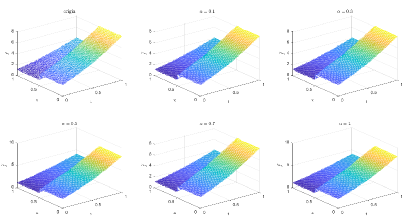
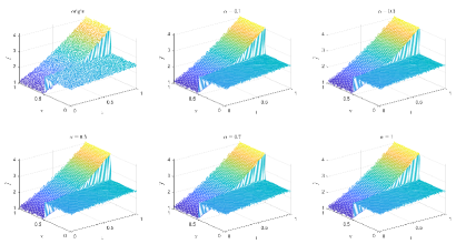
Table 1 and Figures 4-7 show the relative error (6.1) between the source function in Example 1 and discovery in (4.2) with epoch= in Type 1. From Table 1, it can be found that our proposed algorithm is stable and accurate faced with different discretization sizes and noise level, which is robust even for uniformly distributed noise level.
| Threshold | 0.1 | 0.3 | 0.5 | 0.7 | 1 | |
|---|---|---|---|---|---|---|
| noise | 1/25 | 1.3898e-01 | 1.3898e-01 | 1.3898e-01 | 1.3898e-01 | 1.3898e-01 |
| 1/50 | 8.1201e-02 | 8.1201e-02 | 8.1201e-02 | 8.1201e-02 | 8.1201e-02 | |
| 1/100 | 3.4951e-02 | 3.4951e-02 | 3.4951e-02 | 3.4951e-02 | 3.4951e-02 | |
| noise | 1/25 | 1.4190e-01 | 1.4190e-01 | 1.4190e-01 | 1.4190e-01 | 1.4190e-01 |
| 1/50 | 8.2515e-02 | 8.2515e-02 | 8.2515e-02 | 8.2515e-02 | 8.2515e-02 | |
| 1/100 | 1.6557e-02 | 1.6557e-02 | 1.6557e-02 | 1.6557e-02 | 1.6557e-02 | |
| noise | 1/25 | 1.3998e-01 | 1.3998e-01 | 1.3998e-01 | 1.3998e-01 | 1.3998e-01 |
| 1/50 | 8.1266e-02 | 8.1266e-02 | 8.1266e-02 | 8.1266e-02 | 8.1266e-02 | |
| 1/100 | 8.1891e-03 | 8.1891e-03 | 8.1891e-03 | 8.1891e-03 | 8.1891e-03 | |
| clean data | 1/25 | 1.2192e-01 | 1.2192e-01 | 1.2192e-01 | 1.2192e-01 | 1.2192e-01 |
| 1/50 | 8.1341e-02 | 8.1341e-02 | 8.1341e-02 | 8.1341e-02 | 8.1341e-02 | |
| 1/100 | 3.1629e-03 | 3.1629e-03 | 3.1629e-03 | 3.1629e-03 | 3.1629e-03 |
6.1.2 Type 2 in DNN
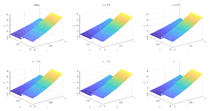
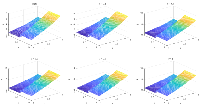
Table 2 and Figures 8-11 show the relative error (6.1) between the source function in Example 1 and discovery in (4.2) with epoch= in Type 2. The numerical experiments are given to illustrate the availability using deep learning. In fact, from Table 2, it can be found that our proposed algorithm is stable and accurate faced with different discretization sizes and noise level, and is also robust even for uniformly distributed noise level.
| Threshold | 0.1 | 0.3 | 0.5 | 0.7 | 1 | |
|---|---|---|---|---|---|---|
| noise | 1/25 | 1.0774e-01 | 1.0659e-01 | 1.0676e-01 | 1.0695e-01 | 1.0952e-01 |
| 1/50 | 7.9438e-02 | 7.9069e-02 | 7.9516e-02 | 7.9440e-02 | 8.1030e-02 | |
| 1/100 | 5.2110e-02 | 5.1856e-02 | 5.1991e-02 | 5.2098e-02 | 5.2704e-02 | |
| noise | 1/25 | 1.1791e-01 | 1.1925e-01 | 1.1919e-01 | 1.1859e-01 | 1.1716e-01 |
| 1/50 | 7.9669e-02 | 8.0419e-02 | 8.0401e-02 | 7.9954e-02 | 7.9223e-02 | |
| 1/100 | 1.5546e-02 | 1.5030e-02 | 1.5171e-02 | 1.4991e-02 | 1.6229e-02 | |
| noise | 1/25 | 1.2006e-01 | 1.2129e-01 | 1.2091e-01 | 1.2068e-01 | 1.2047e-01 |
| 1/50 | 8.0694e-02 | 8.1230e-02 | 8.1086e-02 | 8.0716e-02 | 8.0783e-02 | |
| 1/100 | 1.0260e-02 | 9.6543e-03 | 9.5003e-03 | 9.5757e-03 | 1.0225e-02 | |
| clean data | 1/25 | 1.2154e-01 | 1.2198e-01 | 1.2206e-01 | 1.2179e-01 | 1.2169e-01 |
| 1/50 | 8.1152e-02 | 8.1369e-02 | 8.1410e-02 | 8.1255e-02 | 8.1141e-02 | |
| 1/100 | 4.8904e-03 | 3.7653e-03 | 3.7053e-03 | 3.6545e-03 | 4.7890e-03 |
Example 2
Let us consider the following subdiffusion problem (1.1) with uniform noise
where the source function with the random noise is given by
Here is the uniform noise with (clean data) , , level for a single uniform distributed random number in the interval , respectively. In this experiment, we train the deep learning discovery in (4.2).
6.1.3 Type 1 in DNN
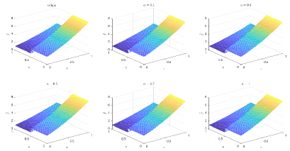
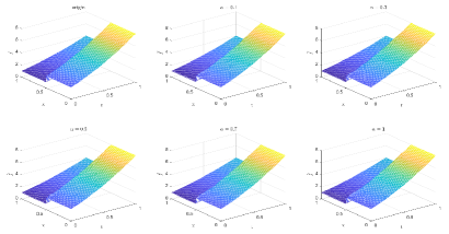
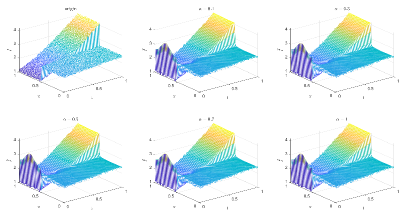
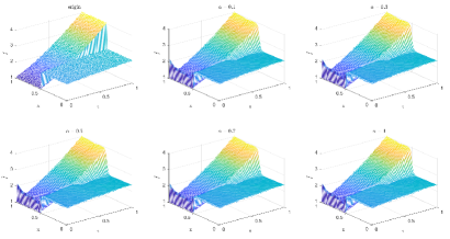
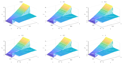
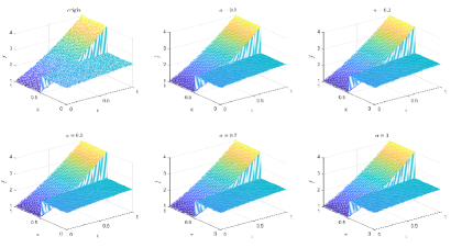
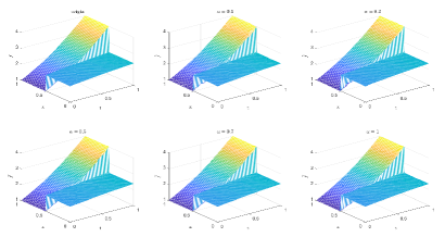
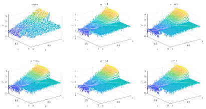
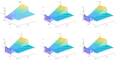
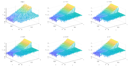
Table 3 and Figures 12-15 show the relative error (6.1) between the source function in Example 2 and discovery in (4.2) with different noise levels and epoch= in Type 1. The numerical experiments are given to illustrate the availability using deep learning for the different noise levels. From Table 3, it can be found that our proposed algorithm is stable and accurate faced with different discretization sizes and noise level, which is robust even for uniformly distributed noise level. From Figures 12-15, it appears a layer or blows up at (boundary noise pollution), since the low time regularity ShCh:2020 ; SOG:17 .
| Noise Level | 0.1 | 0.3 | 0.5 | 0.7 | 1 | |
|---|---|---|---|---|---|---|
| noise | 1/25 | 1.5132e-01 | 1.5132e-01 | 1.5132e-01 | 1.5132e-01 | 1.5132e-01 |
| 1/50 | 1.2040e-01 | 1.2040e-01 | 1.2040e-01 | 1.2040e-01 | 1.2040e-01 | |
| 1/100 | 1.1607e-01 | 1.1607e-01 | 1.1607e-01 | 1.1607e-01 | 1.1607e-01 | |
| noise | 1/25 | 1.1360e-01 | 1.1360e-01 | 1.1360e-01 | 1.1360e-01 | 1.1360e-01 |
| 1/50 | 8.3587e-02 | 8.3587e-02 | 8.3587e-02 | 8.3587e-02 | 8.3587e-02 | |
| 1/100 | 6.1966e-02 | 6.1966e-02 | 6.1966e-02 | 6.1966e-02 | 6.1966e-02 | |
| noise | 1/25 | 5.8198e-02 | 5.8198e-02 | 5.8198e-02 | 5.8198e-02 | 5.8198e-02 |
| 1/50 | 4.2641e-02 | 4.2641e-02 | 4.2641e-02 | 4.2641e-02 | 4.2641e-02 | |
| 1/100 | 3.5011e-02 | 3.5011e-02 | 3.5011e-02 | 3.5011e-02 | 3.5011e-02 | |
| clean data | 1/25 | 5.2867e-02 | 5.2867e-02 | 5.2867e-02 | 5.2867e-02 | 5.2867e-02 |
| 1/50 | 3.7670e-02 | 3.7670e-02 | 3.7670e-02 | 3.7670e-02 | 3.7670e-02 | |
| 1/100 | 2.0318e-02 | 2.0318e-02 | 2.0318e-02 | 2.0318e-02 | 2.0318e-02 |
6.1.4 Type 2 in DNN
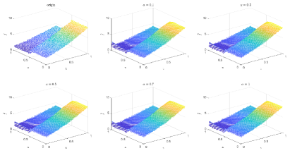
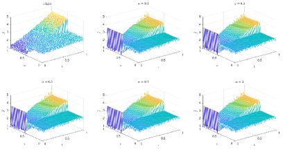
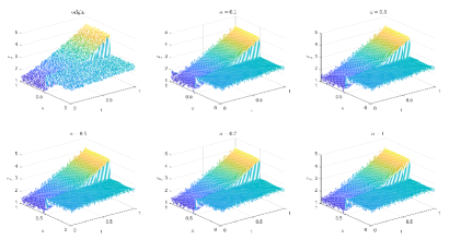
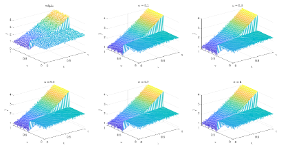
Table 4 and Figures 16-19 show the relative error (6.1) between the source function in Example 1 and discovery in (4.2) with different noise levels and epoch= in Type 2. The numerical experiments are given to illustrate the availability using deep learning for the different noise levels. From Table 4, it can be found that our proposed algorithm is stable and accurate faced with different discretization sizes and noise level, which is robust even for uniformly distributed noise level. From Figures 16-19, it also appears a little layer or blows up at (boundary noise pollution), since the low time regularity ShCh:2020 ; SOG:17 . It seems that Type 2 is better than Type1 from observed data.
| Noise Level | 0.1 | 0.3 | 0.5 | 0.7 | 1 | |
|---|---|---|---|---|---|---|
| noise | 1/25 | 8.6685e-02 | 8.5475e-02 | 8.4797e-02 | 8.4731e-02 | 8.1521e-02 |
| 1/50 | 7.2426e-02 | 7.1836e-02 | 7.1454e-02 | 7.1377e-02 | 6.9543e-02 | |
| 1/100 | 6.2809e-02 | 6.2084e-02 | 6.1725e-02 | 6.1470e-02 | 6.1917e-02 | |
| noise | 1/25 | 6.6977e-02 | 6.7135e-02 | 6.6908e-02 | 6.7067e-02 | 6.7562e-02 |
| 1/50 | 4.8547e-02 | 4.8697e-02 | 4.8523e-02 | 4.8578e-02 | 4.8868e-02 | |
| 1/100 | 2.7690e-02 | 2.7786e-02 | 2.7643e-02 | 2.7814e-02 | 2.7819e-02 | |
| noise | 1/25 | 6.3849e-02 | 6.3655e-02 | 6.3809e-02 | 6.3935e-02 | 6.3953e-02 |
| 1/50 | 4.3969e-02 | 4.3909e-02 | 4.3996e-02 | 4.4066e-02 | 4.4010e-02 | |
| 1/100 | 1.8282e-02 | 1.8648e-02 | 1.8545e-02 | 1.8526e-02 | 1.8353e-02 | |
| clean data | 1/25 | 5.6927e-02 | 5.8353e-02 | 5.8272e-02 | 5.7993e-02 | 5.8502e-02 |
| 1/50 | 3.8296e-02 | 3.9283e-02 | 3.9420e-02 | 3.9318e-02 | 3.9337e-02 | |
| 1/100 | 5.4745e-03 | 4.4494e-03 | 4.9254e-03 | 4.7000e-03 | 3.9269e-03 |
6.2 Numerical Experiments for discovery with Guassian noise
Example 3
Let us consider the Example 2 again with Guassian noise, namely,
where the source function with the random noise is given by
Here is the Guassian noise with (clean data) , , level, respectively, which is statistical noise having a probability density function equal to that of the normal distribution. In this experiment, we train the deep learning discovery in (4.2).
6.2.1 Type 1 in DNN
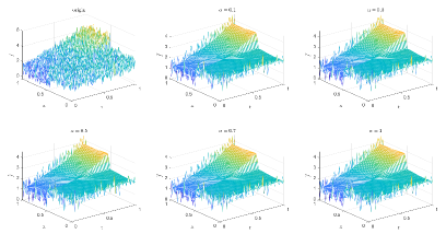
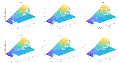
Table 5 and Figures 20-23 show the relative error (6.1) between the source function in Example 2 and discovery in (4.2) with different noise levels and epoch= in Type 1. The numerical experiments are given to illustrate the availability using deep learning for the different noise levels. From Table 5, it can be found that our proposed algorithm is stable and accurate faced with different discretization sizes and noise level, which is robust even for Guassian noise level. From Figures 20-23, it also appears a layer or blows up at (boundary noise pollution).
| Threshold | 0.1 | 0.3 | 0.5 | 0.7 | 1 | |
|---|---|---|---|---|---|---|
| noise | 1/25 | 2.1181e-01 | 2.1181e-01 | 2.1181e-01 | 2.1181e-01 | 2.1181E-01 |
| 1/50 | 2.1048e-01 | 2.1048e-01 | 2.1048e-01 | 2.1048e-01 | 2.1048e-01 | |
| 1/100 | 2.1618e-01 | 2.1618e-01 | 2.1618e-01 | 2.1618e-01 | 2.1618e-01 | |
| noise | 1/25 | 1.1250e-01 | 1.1250e-01 | 1.1250e-01 | 1.1250e-01 | 1.1250e-01 |
| 1/50 | 9.5174e-02 | 9.5174e-02 | 9.5174e-02 | 9.5174e-02 | 9.5174e-02 | |
| 1/100 | 9.1433e-02 | 9.1433e-02 | 9.1433e-02 | 9.1433e-02 | 9.1433e-02 | |
| noise | 1/25 | 1.1917e-01 | 1.1917e-01 | 1.1917e-01 | 1.1917e-01 | 1.1917e-01 |
| 1/50 | 8.6597e-02 | 8.6597e-02 | 8.6597e-02 | 8.6597e-02 | 8.6597e-02 | |
| 1/100 | 7.4511e-02 | 7.4511e-02 | 7.4511e-02 | 7.4511e-02 | 7.4511e-02 | |
| clean data | 1/25 | 7.0042e-02 | 7.0042e-02 | 7.0042e-02 | 7.0042e-02 | 7.0042e-02 |
| 1/50 | 4.0945e-02 | 4.0945e-02 | 4.0945e-02 | 4.0945e-02 | 4.0945e-02 | |
| 1/100 | 1.4316e-02 | 1.4316e-02 | 1.4316e-02 | 1.4316e-02 | 1.4316e-02 |
6.2.2 Type 2 in DNN
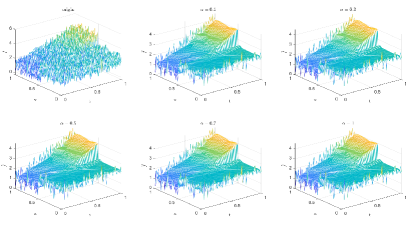
Table 6 and Figures 24-26 show the relative error (6.1) between the source function in Example 2 and discovery in (4.2) with different noise levels and epoch= in Type 2. The numerical experiments are given to illustrate the availability using deep learning for the different noise levels. From Table 6, it can be found that our proposed algorithm is stable and accurate faced with different discretization sizes and noise level, which is robust even for Guassian noise level. From Figures 24-26, it also appears a littlt layer or blows up at (boundary noise pollution).
| Threshold | 0.1 | 0.3 | 0.5 | 0.7 | 1 | |
|---|---|---|---|---|---|---|
| with noise | 1/25 | 2.1509e-01 | 2.1435e-01 | 2.1464e-01 | 2.1482e-01 | 2.1413e-01 |
| 1/50 | 2.1005e-01 | 2.0957e-01 | 2.0972e-01 | 2.0975e-01 | 2.0946e-01 | |
| 1/100 | 2.0500e-01 | 2.0510e-01 | 2.0529e-01 | 2.0529e-01 | 2.0537e-01 | |
| with noise | 1/25 | 1.0418e-01 | 1.0426e-01 | 1.0441e-01 | 1.0465e-01 | 1.0478e-01 |
| 1/50 | 9.2908e-02 | 9.2833e-02 | 9.2892e-02 | 9.3044e-02 | 9.2955e-02 | |
| 1/100 | 8.5171e-02 | 8.4946e-02 | 8.5225e-02 | 8.5757e-02 | 8.8259e-02 | |
| with noise | 1/25 | 7.3662e-02 | 7.4271e-02 | 7.4214e-02 | 7.4147e-02 | 7.4018e-02 |
| 1/50 | 5.7890e-02 | 5.8266e-02 | 5.8156e-02 | 5.8111e-02 | 5.8036e-02 | |
| 1/100 | 4.2822e-02 | 4.2814e-02 | 4.2745e-02 | 4.2785e-02 | 4.2809e-02 | |
| with noise | 1/25 | 5.6927e-02 | 5.8353e-02 | 5.8272e-02 | 5.7993e-02 | 5.8502e-02 |
| 1/50 | 3.8296e-02 | 3.9283e-02 | 3.9420e-02 | 3.9318e-02 | 3.9337e-02 | |
| 1/100 | 5.4745e-03 | 4.4494e-03 | 4.9254e-03 | 4.7000e-03 | 3.9269e-03 |
7 Conclusion
In this work, we firstly propose the discovery of subdiffusion with noisy data in deep learning based on the designing two types. The numerical experiments are given to illustrate the availability using deep learning even for the noise level. The advantage of first Type is that model (4.2) can be trained for each fixed , which reduces the computational count and required storage, since it fixes as input data. Obviously, it may loss some accuracy. To recover the accuracy, second Type is complemented, which needs more computational count. It implies an interesting generalized structure by combining Type 1 and Type 2, which may keep suitable accuracy and reduces computational count. As a result, even when discovering the interger-order equations, the proposed type DNNs have some advantages compared with the traditional numerical scheme and previous works to solve the data-driven discovery for differential equations. The interesting topic is reducing the computational count and storage by fast multigrid or conjugate gradient squared method CCNWL:20 ; CES:20 . Another interesting topic is how to design the correction of approximation for reducing the boundary noise pollution, since subdiffuison model appears a layer or blows up at ShCh:2020 ; SOG:17 with low time regularity.
References
- (1) Cao, R.J., Chen, M.H., Ng, M.K., Wu, Y.J.: Fast and high-order accuracy numerical methods for time-dependent nonlocal problems in . J. Sci. Comput. 84:8 (2020).
- (2) Chen, J.R., Jin, S., Lyu, L.Y.: A Deep learning Based Discotinuous Galerkin Method for Hyperbolic Equations with Discontinuous Solutions and Random Uncertainties. arXiv:2107.01127
- (3) Chen, M.H., Jiang, S.Zh., Bu, W.P.: Two schemes on graded meshes for fractional Feynman-Kac equation. J. Sci. Comput. 88:58 (2021)
- (4) Chen, M.H., Ekström, S.E., Serra-Capizzano, S.: A Multigrid method for nonlocal problems: non-diagonally dominant or Toeplitz-plus-tridiagonal systems. SIAM J. Matrix Anal. Appl. 41 1546-1570 (2020)
- (5) Chen, W.Q., Wang, Q., Hesthaven, J.S., Zhang, C.H.: Physics-informed machine learning for reduced-order modeling of nonlinear problems. J. Comput. Phys. 446, 110666 (2021)
- (6) Eliazar, I., Klafter, J.: Anomalous is ubiquitous. Ann. Physies 326, 2517–2531 (2011)
- (7) Du. Q., Gu, Y.Q., Yang, H.Z., Zhou, C.: The discovery of dynamics via linear multistep methods and deep learning:error estimation. arXiv:2103.11488
- (8) Duan, C.G., Jiao, Y.L, Lai, Y.M., Lu, X.L.,Yang, Z.J.: Convergence rate analysis for deep Ritz method. arXiv:2103.13330
- (9) E, W.N., Yu, B.: The Deep Ritz method:A deep learning-based numerical algorithm for solving variational problems. Commun. Math. Stat. 6, 1–12 (2018)
- (10) Goodfellow, I., Bengio, Y., Courville, A.: Deep Learning. Adaptive Computation and Machine Learning. MIT Press, Cambridge (2016)
- (11) Gu, Y.Q., Ng, M.K.: Deep Ritz method for the spectral fractional Laplacian equation using the Caffarelli-Silvestre extension. arXiv:2108.11592
- (12) Gulian, M.K., Raissi, M., Perdikaris, P., Karniadakis, G.: Machine learning of space-fractional differential equations. SIAM J. Sci. Comput. 41, A2485–A2509 (2019)
- (13) Jiao, Y.L., Lai, Y.M., Lo,Y.S., Wang.Y., Yang.Y.F.: Error Analysis of Deep Ritz Methods for Elliptic Equations. arXiv:2107.14478
- (14) Keller, R., Du, Q.: Discovery of dynamics using linear multistep methods. SIAM J. Numer. Anal. 59, 429–455 (2021)
- (15) Li, Y.J., Wang, Y.J., Deng, W.H.: Galerkin finite element approximations for stochastic space-time fractional wave equations. SIAM J. Numer. Anal. 55, 3173–3202 (2017)
- (16) Li, Z.Y., Kovachki, N., Azizzadenesheli., K., Liu, B. ,Bhattacharya, K., Stuart, A., Anandkumar, A.: Markov Neurl Operators for Learning Chaotic Systems. arXiv:2106.06898
- (17) Lin, Y.M., Xu, C.J.: Finite difference/spectral approximations for the time-fractional diffusion equation. J. Comput. Phys. 225, 1533–1552 (2007)
- (18) Meerschaert, M.M., Sikorskii, A.: Stochastic Models for Fractional Calculus. de Gruyter GmbH Berlin (2012)
- (19) Metzler R., Klafter J.: The random walk’s guide to anomalous diffusion: a fractional dynamics approach. Phys. Rep. 339, 1–77 (2000)
- (20) Podlubny I.: Fractional Differential Equations. Academic Press, New York (1999)
- (21) Qin, T., Wu, K., Xiu, D.: Data driven governing equations approximation using deep neural network. J. Comput. Phys. 395, 620–635 (2019)
- (22) Raissi, M.: Deep hidden physics models deep learning of nonlinear partial differential equations. The Journal of Machine Learning Research. 19, 1–24 (2018)
- (23) Rudy, S.H., Kutz, J.N, Brunton, S.L.: Deep learning of dynamics and signal-noise decompoisition with time-stepping constraints. J. Comput. Phys. 396, 483–506 (2019)
- (24) Shen, Z.W., Yang, H.Z., Zhang, S.J.: Deep Network Approximation Characterized by Number of Neurons Commun. Comput. Phys., 28, 1768–1811 (2019)
- (25) Shen, X., Cheng, X.L., Liang, .K.W.: Deep Euler Method: Solving ODEs by approximating the local truncation error of the euler method. arXiv:2003.09573
- (26) Sirignano, J., Spiliopoulos, K.: DGM: A deep learning algorithm for solving partial differental equations. J. Comput. Phys. 375, 1339–1364 (2018)
- (27) Shi, J.K., Chen, M.H.: Correction of high-order BDF convolution quadrature for fractional Feynman-Kac equation with Lévy flight. J. Sci. Comput. 85:28 (2020)
- (28) Stynes, M., O’riordan, E., Gracia, J.L.: Error analysis of a finite difference method on graded meshes for a time-fractional diffusion equation. SIAM J. Numer. Anal. 55, 1057–1079 (2017)
- (29) Tipireddy, R., Perdikaris, P., Stinis , P., Tartakovsky, A.: A comparative study of physics-informed neural network models for learning unknown dynamics and constitutive relations. arXiv:1904.04058
- (30) Wang, C., Chen, M.H., Deng, W.H., Bu, W.P., Dai, X.J.: A sharp error estimate of Euler–Maruyama method for stochastic Volterra integral equations. Math. Method Appl. Sci. Minor Revised.
- (31) Xu, Y., Zhang, H., Li, Y.G., Zhou, K., Liu, Q., Jurgen, K.: Solving Fokker-Planck equation using deep learning. Chaos. 30, 013133 (2020)
- (32) Zhang, Z.H., Karniadakis, G.E.: Numerical Methods for Stochastic Partial Differential Equations with White Noise. Springer, New York (2017)