DiscQuant: A Quantization Method for
Neural Networks Inspired by Discrepancy Theory
Abstract
Quantizing the weights of a neural network has two steps: (1) Finding a good low bit-complexity representation for weights (which we call the quantization grid) and (2) Rounding the original weights to values in the quantization grid. In this paper, we study the problem of rounding optimally given any quantization grid. The simplest and most commonly used way to round is Round-to-Nearest (RTN). By rounding in a data-dependent way instead, one can improve the quality of the quantized model significantly.
We study the rounding problem from the lens of discrepancy theory, which studies how well we can round a continuous solution to a discrete solution without affecting solution quality too much. We prove that given samples from the data distribution, we can round all but model weights such that the expected approximation error of the quantized model on the true data distribution is as long as the space of gradients of the original model is approximately low rank (which we empirically validate).
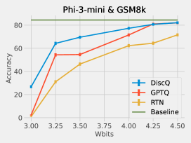
Our proof, which is algorithmic, inspired a simple and practical rounding algorithm called DiscQuant. In our experiments, we demonstrate that DiscQuant significantly improves over the prior state-of-the-art rounding method called GPTQ and the baseline RTN over a range of benchmarks on Phi3mini-3.8B and Llama3.1-8B. For example, rounding Phi3mini-3.8B to a fixed quantization grid with 3.25 bits per parameter using DiscQuant gets 64% accuracy on the GSM8k dataset, whereas GPTQ achieves 54% and RTN achieves 31% (the original model achieves 84%). We make our code available at https://github.com/jerry-chee/DiscQuant.
1 Introduction
Modern deep learning models continue to grow in size, incurring greater challenges to train and serve these models. Post training compression methods have emerged which aim to make model inference faster and cheaper. Compressing after pretraining is desirable among practitioners who either cannot afford to train models themselves, or do not want to change the expensive training process too much. In this paper, we study post training quantization (PTQ) of the model weights. Quantization reduces the memory requirements of the model, and speeds up inference for LLMs under memory-bound settings such as the generation phase (as opposed to prefilling phase which is compute-bound) (Kwon et al., 2023).
The quantization problem can be divided into two overall steps: (1) Construct a good low bit-complexity representation for the weights (we colloquially call this the quantization grid), and (2) Round the original weights to values in the quantization grid. Within step (1), we also consider those methods which apply a transformation on the weights to better match the encoding format. There has been much recent work on weights-only PTQ for LLMs. To date, the vast majority of such research has been focused on step (1): constructing good low bit representations (Shao et al., 2024; Tseng et al., 2024a; Egiazarian et al., 2024). However, work on rounding methods is under-explored. To the best of our knowledge, Round-to-Nearest (RTN) and GPTQ (Hassibi et al., 1993; Frantar et al., 2022, 2023) are the primary rounding methods for LLM weight quantization. RTN is a simple baseline, and GPTQ is a data dependent method which aims to match the activations of the quantized model with that of the original model layer-by-layer.
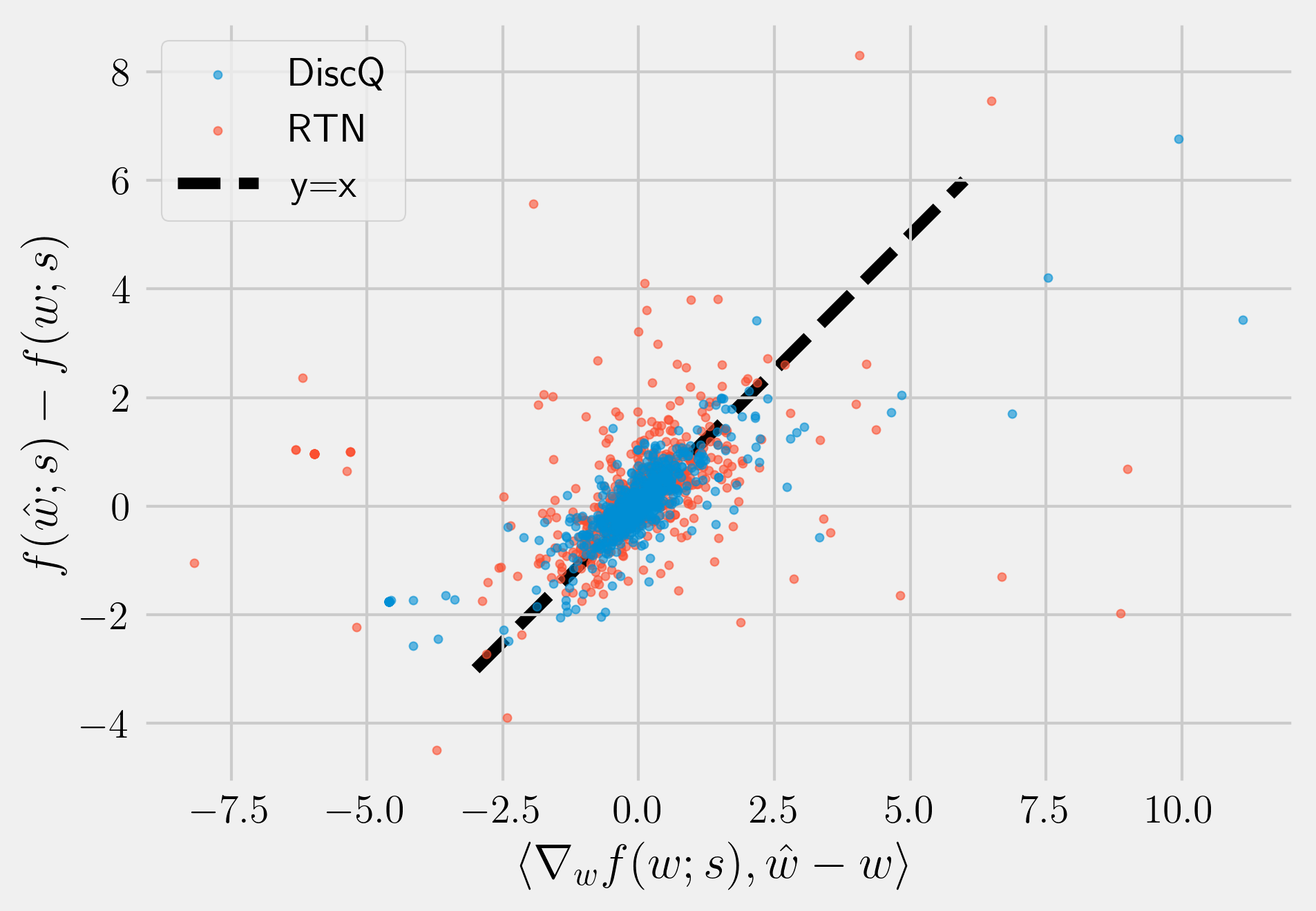
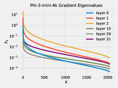
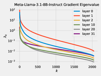
Let be the loss function of a neural network where are original pretrained weights and is an input sample; for example can be the usual cross-entropy loss on input . To find a good rounding solution, we are looking for perturbations of the original weights that correspond to values in the quantization grid, and do not increase the loss too much. We further impose the constraint that we only round each parameter up or down, this ensures that we are not changing the original model weights too much. Then the set of allowed quantization points can be pictured as vertices of a hypercube around . Let be these perturbed weights, and be the resulting change in loss function for a sample . We approximate via a first order Taylor expansion: . Some prior works such as Nagel et al. (2020); Hassibi et al. (1993) assume the gradients of a pretrained model to be nearly zero, and focus on the second order terms. We show that this assumption is not always true, the average gradients are close to zero but per-sample gradients can be big; in fact the first order term is a good approximation to (see Figure 4).
Therefore, to incur a small , we want for sampled from the data distribution . Suppose we are given independent samples , we can impose the constraints which correspond to an affine subspace of dimension . The intersection of the subspace and the hypercube is a convex polytope . It can be shown that any vertex of should have at least fully rounded parameters, see Figure 1 for an illustration. Since the number of parameters , any vertex of gives an almost fully rounded solution. Obviously this solution satisfies the linear constraints for the samples . But will it generalize to unseen samples from the data distribution ? We prove that it can generalize if the distribution of gradients for is approximately low rank. Let where be the covariance matrix of gradients. We prove the following theorem; the algorithm and the proof draws on techniques from discrepancy theory, in particular the famous Lovett-Meka algorithm (Lovett and Meka, 2012).
Theorem 1.1 (Informal).
If the eigenvalues of the covariance matrix of gradients decay polynomially fast, then given samples there is a randomized algorithm to find with weights rounded such that
From these insights we develop a practical rounding algorithm called DiscQuant. The Lovett-Meka algorithm does a random walk starting from the original weights until it converges to a vertex of . Instead, we can find a vertex of by minimizing a linear function over the convex polytope . DiscQuant uses stochastic gradient descent to minimize two objectives, one corresponding to low , and the other corresponding to minimizing a linear function. We take a knowledge distillation approach for the first term, minimizing the KL divergence between the original and quantized model. These two losses are balanced with a regularization parameter :
| (1) | ||||
Here is the next token distribution given prefix . An astute reader may notice that the first order approximation of the KL divergence in (1) is exactly zero, and how our discussion above applies. In Section 4 where we describe in detail our exact optimization objective, we also show that the second order term of KL divergence can be written as
So minimizing the KL divergence is a succinct way to impose constraints of the form or equivalently where and . Therefore our framework still applies.
After every step of gradient descent, we project the weights back to the hypercube . This ensures that the trajectory of DiscQuant remains within the convex polytope and eventually converges to a vertex of with almost all the coordinates rounded. Instead of picking a random direction to find a random vertex of , we use a special which let’s us find the vertex closest to the original weights (see Section 4). We use RTN to round the few unrounded parameters left at the end of the optimization.
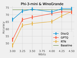
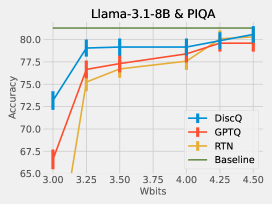
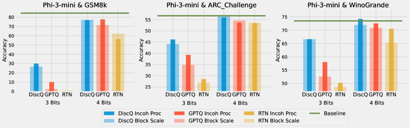
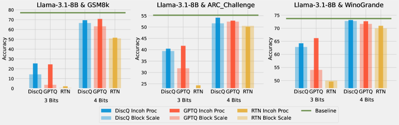
We perform extensive experiments which show the strength of our method: on models Phi-3-mini-4k-instruct and Meta-Llama-3.1-8B-Instruct, across a variety of evaluation tasks, and across the block scaling and incoherence processing quantization formats. DiscQuant is agnostic towards the quantization grid, and can therefore be composed with other quantization methods. Block scaling sets a bits parameter which determines the number of grid points, and a unique scaling parameter per groupsize weights (Frantar et al., 2023). Incoherence processing applies a random orthogonal transformation, which reduces the weight ranges and can make quantization easier (Chee et al., 2023; Tseng et al., 2024a). A subset of results can be found in Figure 2. Across tasks, models, and quantization levels, our method DiscQuant achieves superior compression over baselines GPTQ and RTN.
We summarize our main contributions:
-
•
Theoretical developments: We prove that it is possible to achieve generalization error on the true data distribution by rounding all but weights, so long as the gradients of the original model are approximately low rank.
-
•
Practical algorithm: We develop a simple and practical algorithm DiscQuant guided by our theoretical analysis. We perform extensive experiments on Phi-3-mini-4k-instruct and Meta-Llama-3.1-8B-Instruct, over block scaling and incoherence processing quantization formats, and a variety of evaluation tasks. Our method DiscQuant achieves superior or comparable quantization to the baselines GPTQ and RTN as can be seen from Figure 2.
2 Related Work
In this paper we focus on weights-only PTQ.
Quantization can also be applied to the activations or KV-cache (Ashkboos et al., 2024; Liu et al., 2024a, b).
Other compression method such as pruning
(Frantar and Alistarh, 2023; Sun et al., 2023) are also outside the scope of this work.
As discussed in the introduction, post training quantization can be divided into two overall steps: (1) Construct a good low bit-complexity representations for the weights (the quantization grid), and (2) Round the original weights to the values in the quantization grid.
To this date, the vast majority of PTQ research for LLMs has focused on step (1).
Note that determining a good compressed representation can involve both encoding formats, as well as transformations to ensure the weights better match the encoding format.
2.1 Quantization Grids
One of the more common quantization formats is called block scaling, or group-wise quantization (Frantar et al., 2023). In addition to the bits parameter determining the number of representable points, each groupsize parameters share a unique scaling parameter. Another successful encoding is to identify a small set of important weights and keep them in high precision (Dettmers et al., 2022, 2024; Kim et al., 2024). Shao et al. (2024) learns quantization parameters. Other works apply transformations to make quantization easier, either relatively simple invariant scalings (Xiao et al., 2023; Lin et al., 2024), or more complicated random orthogonal transformations (Chee et al., 2023; Liu et al., 2024a). Beyond block scaling, there has been work quantizing multiple parameters together using vector quantization (Tseng et al., 2024a; Egiazarian et al., 2024; van Baalen et al., 2024) or trellis quantization (Tseng et al., 2024b).
2.2 Rounding
To the best of our knowledge, GPTQ (Frantar et al., 2023) is the main rounding method for LLMs. It is based on the Optimal Brain Surgeon (Hassibi et al., 1993), which was adapted for pruning and quantization in Frantar et al. (2022) and then refined for quantization in GPTQ. GPTQ works by minimizing a layer-wise objective , where is the weight matrix of a linear layer and is the matrix of input activations to that layer (stacked as columns). Two other LLM rounding methods both use coordinate descent: Nair and Suggala (2024) only has results on the closed source PaLM-2 models with no released code, and Behdin et al. (2023) has results on the OPT, BLOOM, and Falcon model families.
There was more work on rounding methods several years ago, before the LLM boom. These papers were typically on smaller vision models. The line of work was started by AdaRound (Nagel et al., 2020) and continuing to AdaQuant (Hubara et al., 2021) and BRECQ (Li et al., 2021) employ a similar approach to ours, optimizing essentially interpolation variables between the closest up() and down() quantization grid points, while adding a concave regularization term to encourage rounding and using a rectified sigmoid to interpolate between and . They also do rounding layer by layer. However our method uses a linear term as a regularizer inspired from our theoretical insights using discrepancy theory and uses simple linear interpolation between and and we round the entire model at once.
2.3 Discrepancy Theory
Discrepancy theory is a deep branch of mathematics and theoretical computer science, and we refer the readers to standard textbooks for more details (Matousek, 2009; Chazelle et al., 2004; Bansal, 2022) To our knowledge, only Lybrand and Saab (2021) makes the connection between discrepancy theory and quantization. However, besides the high level motivational similarities, their work is not directly relevant to ours. Lybrand and Saab (2021) reduce the problem of understanding the error introduced by quantization on the output of a single neuron to a problem in discrepancy, and construct an algorithm for quantizing a single neuron. Their theoretical analysis on the generalization error only applies to quantizing the first layer of a neural network. On the other hand, we use discrepancy theory to understand when the whole network can be approximated by with in the quantization grid, and our theory holds for any network as a whole as long as our assumptions are true.
3 Connections to Discrepancy Theory
| Model | ||
|---|---|---|
| Phi3-mini-128k | 0.1021 | 4.7812 |
| Llama3.1-8B | 1.6328 | 107 |
Let be the loss function of a pre-trained neural network with weights on an input sample and let be the sample data distribution. Suppose we are also given a (scalar) quantization grid where is a finite set of quantization points available to quantize the parameter.111The quantization grid can depend on , like in Block Scaling (Frantar et al., 2023). So ideally, we should write , but we ignore the dependence to simplify notation. In this work, we focus on scalar quantization which allows us to write the quantization grid as a product set, i.e., each parameter can be independently rounded to a finite set of available values. Alternatively, in vector quantization a group of variables are rounded together to one of a finite set of quantization points in , which has been used in some prior works (Tseng et al., 2024a; Egiazarian et al., 2024; van Baalen et al., 2024). Generalizing our method to vector quantizers is an interesting future research direction.
Our goal is to find a rounding of the original weights such where . We further impose the constraint that for each parameter , we only round up or round down to the available values in , i.e., we only have two choices for denoted by where .222If or , we just set or respectively. We make this assumption because we don’t want to change any parameter of the original model too much during quantization, consider it an important property of algorithms we design. Using Taylor expansion:
| (2) |
Assuming that the quantization grid is fine enough and since we only round each parameter up or down, is small and so we can ignore the higher order terms. We claim that the first order term is the dominant term. Prior works such as Nagel et al. (2020); Hassibi et al. (1993); LeCun et al. (1989) have assumed that the first order term can be assumed to be zero because the model is trained to convergence and focused on reducing the second order term. But the model being trained to convergence just means that average gradient over many samples from the distribution is nearly zero. But the gradients still have some variance and gradients w.r.t. individual samples from the data distribution are not approximately zero (see Table 1). Figure 4 demonstrates this by showing that the error term is well-correlated with the first order approximation .333In the special case when is the KL distillation loss between the original model and quantized model, the first order term vanishes exactly. See Section 4 for why this analysis still applies.
So the goal now is to find a rounding such that for samples Suppose we sample samples independently from the data distribution, where . We now break our task into two parts of bounding the empirical error and generalization error as follows:
Question 3.1.
Can we find (with ) such that for all the samples ?
Question 3.2.
Once we find such a , will it generalize to the true data distribution, i.e., will for ? How many samples do we need for this?
3.1 Bounding empirical error (Question 3.1)
For simplicity, let us assume that the quantization grid is uniform and for all where is the distance between grid points. See Appendix C for how to genealize this to non-uniform grids. We will introduce new parameters and define . Note that interpolates between and where if and if . Let be the interpolation point corresponding to the original weights, i.e., . We can rewrite the linear constraints in terms of as follows:
Let be an matrix whose row is given by . Then the linear constraints can be simply written as . Our goal is to find a fully integral such that Let which is an affine subspace of dimension . Define as the intersection of the hypercube with this subspace. is a convex polytope and it is non-empty because Therefore any vertex of should have integral coordinates (i.e., coordinates such that ).444This is because at a vertex, we need to have tight constraints, and imposes only tight constraints. So the remaining tight constraints should come from the hypercube. These are also called basic feasible solutions in linear programming.
See Figure 1 for geometric intuition about why this is true. Since the number of parameters is much larger than the number of samples , any vertex of is almost fully integral and exactly satisfies all the linear constraints.
Suppose we further ask for a fully integral which approximately satisfies all the linear constraints, this precise question is answered by discrepancy theory which studies how to do this and relates the approximation error to properties of such as hereditary discrepancy (Lovász et al., 1986; Bansal, 2022). We don’t explore this direction further because the almost integral —a vertex of —is good enough if we apply RTN to the few remaining fractional parameters; we observe that the linear constraints are all approximately satisfied.
3.2 Bounding Generalization Error (Question 3.2)
How do we bound the generalization error if we know that the empirical approximation error is small? If is approximately orthogonal to sample gradients for to , why should we expect that is orthogonal to unseen gradients for samples ? This should happen only if the gradients are approximately low rank. More precisely, let
be the covariance matrix of the distribution of sample gradients and let be its eigenvalues. We observe that the eigenvalues decay very fast, see Figure 4 for empirical validation of this on some real world models. We model this by assuming that for . The assumption that is valid since
It is well-known that the gradients of a pretrained model have constant norm on most samples (see Table 1 for empirical validation). Therefore and so the the decay coefficient has to be at least 1.
Under this assumption, it is reasonable to expect generalization. But this is not at all obvious to find a generalizing solution. In fact, any deterministic algorithm which chooses one of the vertices of will most likely not generalize. We give a randomized rounding algorithm (see Algorithm B.2) based on the famous Lovett-Meka algorithm from discrepancy theory (Lovett and Meka, 2012) which finds a vertex of which has low generalization error. The algorithm starts at and does a random walk (Brownian motion) inside the dimensional subspace formed by the linear constraints imposed by the samples. Whenever it hits a face or of the hypercube, it fixes that variable and continues the random walk until almost all the variables are rounded.
In order to prove rigorous bounds we also need a mild assumption that the distribution of gradients is well-behaved. We use the notion by O’Donnell (2014) and say that for a parameter , a random vector is -reasonable if
For example and a Gaussian are both -reasonable. Our main theoretical result (proved in Appendix B) is then:
Theorem 3.3.
Let and be constants and let . Let be a -reasonable distribution with unknown covariance matrix whose Eigenvalues satisfy for all . Then there is a randomized polynomial time algorithm that given a and independent samples , produces an with high probability such that all but parameters in are fully rounded and
4 DiscQuant: Algorithm
In this section, we will present DiscQuant, a simple and practical algorithm for rounding inspired by the theoretical insights in Section 3. Instead of trying to approximate the loss function of the pre-trained model, i.e., , we will instead take a distillation approach and try to minimize the KL divergence between the next token distribution of the original model and the quantized model. Let be the distribution of the next token predicted by the original model given prefix where is a sample from the data distribution. We want .
Expanding using Taylor series, we can see that first order term vanishes exactly and so the second order term is the dominant term (see Appendix D). By Lemma D.1, Hessian of can be written as a covariance of gradients as:
Therefore
So minimizing is a succinct way to impose constraints of the form or equivalently where and . Therefore, we can use the same techniques developed in Section 3 to solve this as well. Assuming that the gradients are low rank, the set of satisfying these constraints (where ) form an affine subspace of dimension where is the number of samples. We are again interested in finding a vertex of the polytope which will have integral coordinates. At this point, we could use the Lovett-Meka algorithm (Algorithm B.2) which has provable generalization guarantees. But explicitly calculating all the gradients and storing them is infeasible. Instead a simple heuristic way to find a random vertex of polytope is to minimize a random linear function. Let be some arbitrary vector; we will try to minimize the linear function along with the KL divergence by taking a linear combination of them. The final optimization objective is shown in (3) where is a regularization coefficient.
| (3) | ||||
We solve the optimization problem (3) using projected stochastic gradient descent where we project to the hypercube after every gradient update. Optimizing (3) will keep us close the polytope and will approximately converge to a vertex of which is almost integral. We round whatever fractional coordinates are left using RTN to get a fully integral solution.
We use one additional heuristic to improve the performance of the algorithm in practice. Instead of choosing a random vertex of the polytope by choosing the vector at random, we will choose it carefully so as to find the vertex of the polytope which is closest to which is the interpolation point corresponding to the original model weights (i.e., such that ). We have:
where . Here we have used the fact that whenever and since is almost integral, we can use the approximation in the summation above. With this approximation, minimizing over almost integral is equivalent to minimizing . So in the DiscQuant algorithm, we use specifically instead of a random
5 Experiments
We evaluate our method on the Phi-3-mini-4k-instruct (Abdin et al., 2024) and Meta-Llama-3.1-8B-Instruct (Dubey et al., 2024) models, and compare against GPTQ and greedy rounding (i.e. round-to-nearest, or RTN). We use the lm-evaluation-harness Gao et al. (2023) to evaluate on the Wikitext, GSM8k_cot 8-shot, MMLU 5-shot, ARC_Challenge 0-shot, PIQA 0-shot, HellaSwag 0-shot, and Winogrande 0-shot tasks. We report standard errors from lm-evaluation-harness. Wikitext measures perplexity, GSM8k is a generative task, and the remaining are multiple choice tasks. Note that generative tasks are typically more difficult than multiple choice tasks, and better reflect how the models are used in practice. See Appendix A for details on the hardware used, and hyper-parameter settings. Our method has similar memory requires as knowledge distillation, which also requires two copies of the model. We do not perform inference timing experiments; DiscQuant can optimize over a given quantization grid, so that we can utilize any pre-existing inference optimizations. For example, there are inference kernels for block scaling (Frantar et al., 2024) and incoherence processing (Tseng et al., 2024a). Ablations on the loss formulation are in Appendix A.
| Method | Wbits | Wiki | GSM8k | MMLU | ArcC | PIQA | Hella | Wino |
|---|---|---|---|---|---|---|---|---|
| — | 16.0 | 9.5 | 84.41.0 | 70.40.4 | 56.71.4 | 80.80.9 | 77.40.4 | 73.51.2 |
| RTN | 3.0 | E | 1.00.3 | 23.30.4 | 26.91.3 | 53.41.2 | 28.20.4 | 48.61.4 |
| GPTQ | 3.0 | 28.2 | 2.30.4 | 37.70.4 | 34.81.4 | 64.31.1 | 56.50.5 | 52.61.4 |
| DiscQ | 3.0 | 17.7 | 26.81.2 | 45.60.4 | 44.11.5 | 73.91.0 | 63.30.5 | 66.61.3 |
| RTN | 3.25 | 22.5 | 31.01.3 | 53.20.4 | 48.41.5 | 72.51.0 | 68.30.5 | 62.61.4 |
| GPTQ | 3.25 | 13.8 | 54.31.4 | 59.00.4 | 49.61.5 | 77.31.0 | 71.10.5 | 66.51.3 |
| DiscQ | 3.25 | 12.6 | 64.21.3 | 60.70.4 | 53.51.5 | 78.71.0 | 72.30.4 | 72.51.3 |
| RTN | 3.5 | 18.8 | 46.31.4 | 57.00.4 | 46.21.5 | 73.81.0 | 70.00.5 | 63.91.4 |
| GPTQ | 3.5 | 12.8 | 54.61.4 | 61.70.4 | 51.61.5 | 78.91.0 | 72.30.4 | 68.31.3 |
| DiscQ | 3.5 | 12.0 | 69.51.3 | 63.00.4 | 51.11.5 | 78.91.0 | 73.00.4 | 73.91.2 |
| RTN | 4.0 | 14.6 | 62.21.3 | 61.20.4 | 53.61.5 | 76.31.0 | 72.90.4 | 65.31.3 |
| GPTQ | 4.0 | 11.5 | 71.51.2 | 65.10.4 | 54.61.5 | 78.81.0 | 74.70.4 | 70.91.3 |
| DiscQ | 4.0 | 11.2 | 77.31.2 | 65.70.4 | 56.81.4 | 79.50.9 | 74.50.4 | 72.01.3 |
| RTN | 4.25 | 11.2 | 64.41.3 | 67.50.4 | 55.51.5 | 79.30.9 | 76.10.4 | 69.11.3 |
| GPTQ | 4.25 | 10.3 | 81.01.1 | 68.50.4 | 56.91.4 | 79.70.9 | 76.10.4 | 72.11.3 |
| DiscQ | 4.25 | 10.2 | 80.71.1 | 68.40.4 | 57.31.4 | 80.70.9 | 76.30.4 | 74.21.2 |
| RTN | 4.5 | 10.8 | 71.61.2 | 67.70.4 | 57.51.4 | 79.30.9 | 76.60.4 | 72.21.3 |
| GPTQ | 4.5 | 10.1 | 82.01.1 | 68.80.4 | 55.81.5 | 80.80.9 | 76.50.4 | 71.81.3 |
| DiscQ | 4.5 | 10.0 | 82.11.1 | 68.50.4 | 56.61.4 | 80.20.9 | 76.70.4 | 74.21.2 |
| Method | Wbits | Wiki | GSM8k | MMLU | ArcC | PIQA | Hella | Wino |
|---|---|---|---|---|---|---|---|---|
| — | 16.0 | 8.7 | 77.01.2 | 68.00.4 | 55.21.5 | 81.30.9 | 79.30.4 | 73.71.2 |
| RTN | 3.0 | E | 0.50.2 | 23.20.4 | 22.31.2 | 52.41.2 | 29.10.5 | 50.01.4 |
| GPTQ | 3.0 | 23.2 | 3.60.5 | 24.60.4 | 31.81.4 | 66.61.1 | 45.80.5 | 54.11.4 |
| DiscQ | 3.0 | 15.2 | 14.31.0 | 44.60.4 | 39.41.4 | 73.21.0 | 64.40.5 | 62.81.4 |
| RTN | 3.25 | 15.2 | 10.80.9 | 50.50.4 | 44.31.5 | 75.21.0 | 71.40.5 | 67.21.3 |
| GPTQ | 3.25 | 10.7 | 56.31.4 | 60.50.4 | 46.31.5 | 76.71.0 | 74.40.4 | 68.71.3 |
| DiscQ | 3.25 | 10.5 | 58.31.4 | 60.20.4 | 49.11.5 | 79.10.9 | 75.10.4 | 72.11.3 |
| RTN | 3.5 | 12.7 | 35.91.3 | 51.40.4 | 48.41.5 | 76.71.0 | 73.00.4 | 69.11.3 |
| GPTQ | 3.5 | 10.4 | 57.01.4 | 62.10.4 | 49.91.5 | 77.31.0 | 75.10.4 | 71.11.3 |
| DiscQ | 3.5 | 10.3 | 60.71.3 | 60.90.4 | 51.71.5 | 79.20.9 | 76.30.4 | 72.51.3 |
| RTN | 4.0 | 12.5 | 50.81.4 | 59.30.4 | 50.51.5 | 77.61.0 | 74.70.4 | 69.91.3 |
| GPTQ | 4.0 | 9.9 | 63.21.3 | 64.40.4 | 52.41.5 | 78.41.0 | 75.90.4 | 71.71.3 |
| DiscQ | 4.0 | 9.8 | 66.51.3 | 63.40.4 | 51.61.5 | 79.20.9 | 76.90.4 | 72.81.3 |
| RTN | 4.25 | 9.4 | 70.61.3 | 65.70.4 | 54.21.5 | 80.10.9 | 78.00.4 | 73.91.2 |
| GPTQ | 4.25 | 9.1 | 74.61.2 | 66.80.4 | 53.41.5 | 79.60.9 | 77.90.4 | 73.51.2 |
| DiscQ | 4.25 | 9.1 | 74.91.2 | 66.90.4 | 53.61.5 | 79.90.9 | 78.40.4 | 72.61.3 |
| RTN | 4.5 | 9.3 | 71.91.2 | 65.80.4 | 54.81.5 | 80.30.9 | 78.40.4 | 72.41.3 |
| GPTQ | 4.5 | 9.0 | 73.81.2 | 66.90.4 | 53.61.5 | 79.60.9 | 78.10.4 | 73.71.2 |
| DiscQ | 4.5 | 9.1 | 74.81.2 | 66.80.4 | 54.11.5 | 80.60.9 | 78.70.4 | 72.91.2 |
5.1 Block Scaling
Our first experiments use standard block scaling quantization, determined by a bits and groupsize parameter. There are unique points, and every groupsize parameters share a unique 16-bit scale parameter. For example, 3.25 bits is achieved with bits=3, groupsize=64. We use the block scaling implementation from Frantar et al. (2024) which is symmetric linear quantization. Table 2 shows the results quantizing Phi-3-mini-4k-instruct. Across all tasks and all bit settings, our method DiscQuant achieves superior or comparable compression over the baseline GPTQ and RTN methods. The gap between DiscQuant and the baselines is greater at lower bits. On the ARC_Challenge, PIQA, and WinoGrade tasks, DiscQuant achieves full recovery with at least 0.25 fewer bits per parameter than GPTQ and RTN. For example on ARC_Challenge, DiscQuant achieves full recovery at 4 bits per weight, whereas GPTQ requires 4.25 bits, and RTN 4.5 bits. DiscQuant achieves better compression on the more difficult generative GSM8k task: at 4 bits DiscQuant gets 77.3% accuracy, while GPTQ gets 71.5%, and RTN gets 62.2%. Table 3 shows the results quantizing Meta-Llama-3.1-8B-Instruct. Overall the story is the same. Our method DiscQuant achieves improved compression on the majority of quantization levels and tasks. For example at 4 bits, DiscQuant gets 66.5% GSM8k accuracy, while GPTQ gets 63.2%, and RTN gets 50.8%.
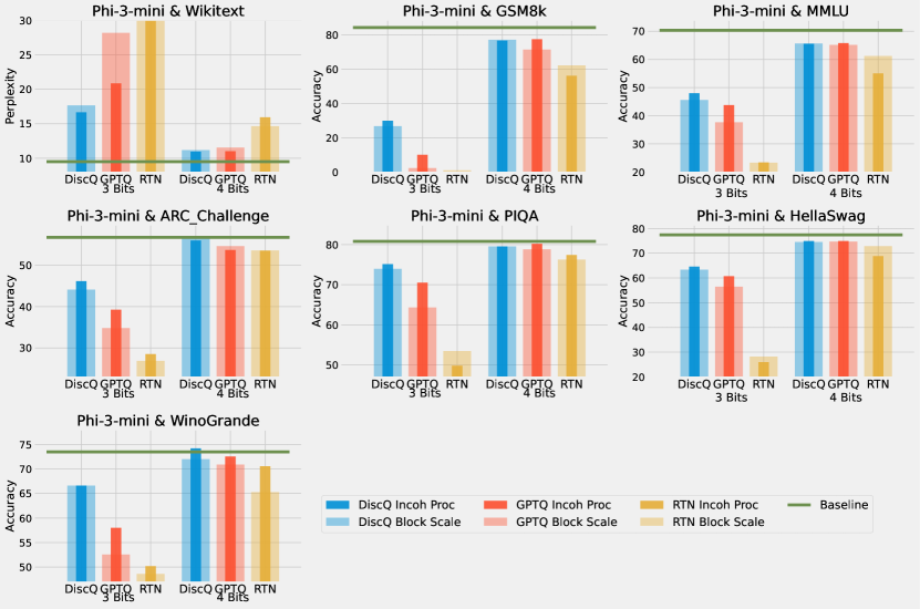
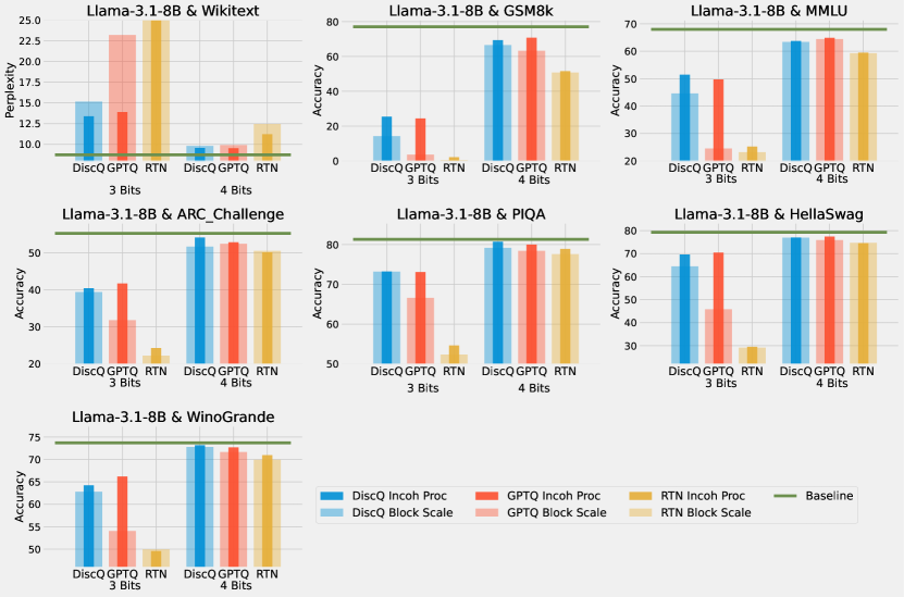
5.2 Incoherence Processing
We explore another quantization format to show that our method can compose with other quantization improvements. Incoherence processing has been shown to improve quantization, especially at less than 4 bits per weight (Chee et al., 2023). The weights are multiplied by certain random orthogonal matrices prior to quantization, which can reduce the range of the weights and make quantization easier. We employ the Randomized Hadamard Transform from Tseng et al. (2024a). We use the same block scaling quantization grid as in the previous subsection. A subset of our results are shown in Figure 5, where we superimpose bar plots for block scaling and block scaling + incoherence processing. In the majority of cases, adding incoherence processing increases the task accuracy, especially at lower bits. We do not use fractional bits, (i.e. no groupsize), due to the fact that both these methods effect outliers and can interfere with one another. Incoherence especially helps GPTQ at 3 bits, and for Phi-3 DiscQuant without incoherence is competitive to GPTQ with incoherence. For full results see Appendix A.

5.3 Effect of Data
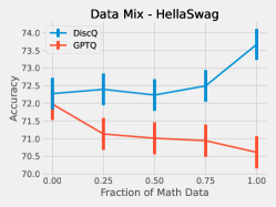
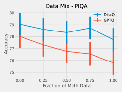
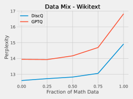
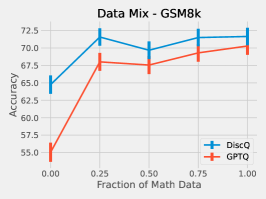
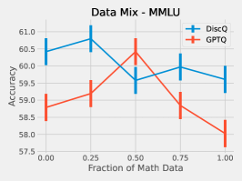
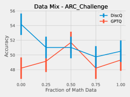
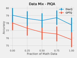
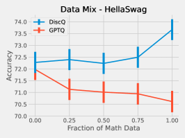
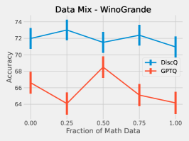
We perform a simple investigation into the effect of the dataset on quantization. We mix math subject data–GSM8k and MetaMathQA–with our standard RedPajama dataset. Figure 6 shows the results of quantizing Phi-3-mini-4k-instruct at 3.25 bits with such a mix. As expected, both methods increase accuracy on GSM8k when there is a greater fraction of math data. On HellaSwag, DiscQuant improves with more math data, where GPTQ gets worse. On PIQA, both methods get worse. See Appendix A for all tasks. There is a meaningful change in accuracy as a result of changing the data mix. Choosing an appropriate data mix for quantization remains an important open question.
References
- Abdin et al. (2024) Marah Abdin, Jyoti Aneja, Hany Awadalla, Ahmed Awadallah, Ammar Ahmad Awan, Nguyen Bach, Amit Bahree, Arash Bakhtiari, Jianmin Bao, and Harkirat Behl. Phi-3 technical report: A highly capable language model locally on your phone, 2024. URL https://arxiv.org/abs/2404.14219.
- Ashkboos et al. (2024) Saleh Ashkboos, Amirkeivan Mohtashami, Maximilian L Croci, Bo Li, Martin Jaggi, Dan Alistarh, Torsten Hoefler, and James Hensman. Quarot: Outlier-free 4-bit inference in rotated llms. In Thirty-either Conference on Neural Information Processing Systems, 2024.
- Bansal (2022) Nikhil Bansal. Discrepancy theory and related algorithms. In Proc. Int. Cong. Math, volume 7, pages 5178–5210, 2022.
- Behdin et al. (2023) Kayhan Behdin, Ayan Acharya, Aman Gupta, Sathiya Keerthi, Rahul Mazumder, Zhu Siyu, and Song Qingquan. Quantease: Optimization-based quantization for language models–an efficient and intuitive algorithm. arXiv preprint arXiv:2309.01885, 2023.
- Chazelle et al. (2004) Bernard Chazelle, William WL Chen, and Anand Srivastav. Discrepancy theory and its applications. Oberwolfach Reports, 1(1):673–722, 2004.
- Chee et al. (2023) Jerry Chee, Yaohui Cai, Volodymyr Kuleshov, and Christopher De Sa. QuIP: 2-bit quantization of large language models with guarantees. In Thirty-seventh Conference on Neural Information Processing Systems, 2023. URL https://openreview.net/forum?id=xrk9g5vcXR.
- Computer (2023) Together Computer. Redpajama: An open source recipe to reproduce llama training dataset, 2023. URL https://github.com/togethercomputer/RedPajama-Data.
- Dettmers et al. (2022) Tim Dettmers, Mike Lewis, Younes Belkada, and Luke Zettlemoyer. Llm.int(): 8-bit matrix multiplication for transformers at scale. In Advances in Neural Information Processing Systems, 2022.
- Dettmers et al. (2024) Tim Dettmers, Ruslan Svirschevski, Vage Egiazarian, Denis Kuznedelev, Elias Frantar, Saleh Ashkboos, Alexander Borzunov, Torsten Hoefler, and Dan Alistarh. Spqr: A sparse-quantized representation for near-lossless llm weight compression, 2024.
- Dubey et al. (2024) Abhimanyu Dubey, Abhinav Jauhri, Abhinav Pandey, Abhishek Kadian, Ahmad Al-Dahle, Aiesha Letman, Akhil Mathur, Alan Schelten, Amy Yang, Angela Fan, et al. The llama 3 herd of models, 2024. URL https://arxiv.org/abs/2407.21783.
- Egiazarian et al. (2024) Vage Egiazarian, Andrei Panferov, Denis Kuznedelev, Elias Frantar, Artem Babenko, and Dan Alistarh. Extreme compression of large language models via additive quantization. In Forty-First International Conference on Machine Learning, 2024.
- Frantar and Alistarh (2023) Elias Frantar and Dan Alistarh. Sparsegpt: Massive language models can be accurately pruned in one-shot. In Proceedings of the International Conference on Machine Learning, 2023.
- Frantar et al. (2022) Elias Frantar, Sidak Pal Singh, and Dan Alistarh. Optimal brain compression: A framework for accurate post-training quantization and pruning. In Advances in Neural Information Processing Systems, 2022.
- Frantar et al. (2023) Elias Frantar, Saleh Ashkboos, Torsten Hoefler, and Dan Alistarh. OPTQ: Accurate quantization for generative pre-trained transformers. In The Eleventh International Conference on Learning Representations, 2023.
- Frantar et al. (2024) Elias Frantar, Roberto L Castro, Jiale Chen, Torsten Hoefler, and Dan Alistarh. Marlin: Mixed-precision auto-regressive parallel inference on large language models. arXiv preprint arXiv:2408.11743, 2024.
- Gao et al. (2023) Leo Gao, Jonathan Tow, Baber Abbasi, Stella Biderman, Sid Black, Anthony DiPofi, Charles Foster, Laurence Golding, Jeffrey Hsu, Alain Le Noac’h, Haonan Li, Kyle McDonell, Niklas Muennighoff, Chris Ociepa, Jason Phang, Laria Reynolds, Hailey Schoelkopf, Aviya Skowron, Lintang Sutawika, Eric Tang, Anish Thite, Ben Wang, Kevin Wang, and Andy Zou. A framework for few-shot language model evaluation, 12 2023. URL https://zenodo.org/records/10256836.
- Hassibi et al. (1993) Babak Hassibi, Daivd G Stork, and Gregory J Wolff. optimal brain surgeon and general network pruning. In IEEE International Conference on Neural Networks, 1993.
- Hubara et al. (2021) Itay Hubara, Yury Nahshan, Yair Hanami, Ron Banner, and Daniel SOudry. Accurate post training quantization with small calibration sets. In Thirty-Eighth International Conference on Machine Learning, 2021.
- Kim et al. (2024) Sehoon Kim, Coleman Hooper, Amir Gholami, Zhen Dong, Xiuyu Li, Sheng Shen, Michael Mahoney, and Kurt Keutzer. Squeezellm: Dense-and-sparse quantization. In Forty-First International Conference on Machine Learning, 2024.
- Kurtic et al. (2023) Eldar Kurtic, Denis Kuznedelev, Elias Frantar, Michael Goin, and Dan Alistarh. Sparse fine-tuning for inference acceleration of large language models, 2023. URL https://arxiv.org/abs/2310.06927.
- Kwon et al. (2023) Woosuk Kwon, Zhuohan Li, Siyuan Zhuang, Ying Sheng, Lianmin Zheng, Cody Hao Yu, Joseph Gonzalez, Hao Zhang, and Ion Stoica. Efficient memory management for large language model serving with pagedattention. In Proceedings of the 29th Symposium on Operating Systems Principles, pages 611–626, 2023.
- LeCun et al. (1989) Yann LeCun, John Denker, and Sara Solla. Optimal brain damage. Advances in neural information processing systems, 2, 1989.
- Li et al. (2021) Yuang Li, Ruihao Gong, Xu Tan, Yang Yang, Peng Hu, Qi Zhang, Fengwei Yu, Wei Wang, and Shi Gu. Brecq: Pushing the limit of post-training quantization by block reconstruction. In The Nineth International Conference on Learning Representations, 2021.
- Lin et al. (2024) Jin Lin, Jiaming Tang, Haotian Tang, Shang Yang, Wei-Ming Chen, Wei-Chen Wang, Guangxuan Xiao, Xingyu Dang, Chuang Gan, and Song Han. Awq: Acttivation-aware weight quantization for on-device llm compression and acceleration. In Seventh Conference on Machine Learning and Systems, 2024.
- Liu et al. (2024a) Zechun Liu, Changsheng Zhao, Igor Fedorov, Bilge Soran, Dhruv Choudhary, Raghuraman Krishnamoorthi, Vikas Chandra, Yuandong Tian, and Tijmen Blankevoort. Spinquant–llm quantization with learned rotations. arXiv preprint arXiv:2405.16406, 2024a.
- Liu et al. (2024b) Zirui Liu, Jiayi Yuan, Hongye Jin, Shaochen Zhong, Zhaozhuo Xu, Vladimir Braverman, Beidi Chen, and Xia Hu. Kivi: A tuning-free asymmetric 2bit quantization for kv cache. In Forty-First International Conference on Machine Learning, 2024b.
- Loshchilov and Hutter (2019) Ilya Loshchilov and Frank Hutter. Decoupled weight decay regularization. The International Conference on Learning Representations, 2019.
- Lovász et al. (1986) László Lovász, Joel Spencer, and Katalin Vesztergombi. Discrepancy of set-systems and matrices. European Journal of Combinatorics, 7(2):151–160, 1986.
- Lovett and Meka (2012) Shachar Lovett and Raghu Meka. Constructive discrepancy minimization by walking on the edges. In FOCS, pages 61–67. IEEE Computer Society, 2012.
- Lybrand and Saab (2021) Eric Lybrand and Rayan Saab. A greedy algorithm for quantizing neural networks. Journal of Machine Learning Research, 22(156):1–38, 2021.
- Matousek (2009) Jiri Matousek. Geometric discrepancy: An illustrated guide, volume 18. Springer Science & Business Media, 2009.
- Nagel et al. (2020) Markus Nagel, Rana Ali Amjad, Mart Van Baalen, Christos Louizos, and Tijmen Blankevoort. Up or down? Adaptive rounding for post-training quantization. In Hal Daumé III and Aarti Singh, editors, Proceedings of the 37th International Conference on Machine Learning, volume 119 of Proceedings of Machine Learning Research, pages 7197–7206. PMLR, 13–18 Jul 2020. URL https://proceedings.mlr.press/v119/nagel20a.html.
- Nair and Suggala (2024) Pranav Ajit Nair and Arun Sai Suggala. Cdquant: Accurate post-training weight quantization of large pre-trained models using greedy coordinate descent, 2024. URL https://arxiv.org/abs/2406.17542.
- O’Donnell (2014) Ryan O’Donnell. Analysis of Boolean Functions. Cambridge University Press, 2014.
- Shao et al. (2024) Wenqi Shao, Mengzhao Chen, Zhaoyang Zhang, Peng Xu, Lirui Zhao, Zhiqian Li, Kaipeng Zhang, Peng Gao, Yu Qiao, and Ping Luo. Omniquant: Omnidirectionally calibrated quantization for large language models. In The Twelfth International Conference on Learning Representations, 2024. URL https://openreview.net/forum?id=8Wuvhh0LYW.
- Sun et al. (2023) Mingjie Sun, Zhuang Liu, Anna Bair, and J Zico Kolter. A simple and effective pruning approach for large language models. In Workshop on Efficient Systems for Foundation Models @ ICML2023, 2023. URL https://openreview.net/forum?id=tz9JV2PRSv.
- Tseng et al. (2024a) Albert Tseng, Jerry Chee, Qingyao Sun, Volodymyr Kuleshov, and Christopher De Sa. QuIP#: Even better llm quantization with hadamard incoherence and lattice codebooks. In Forty-First International Conference on Machine Learning, 2024a.
- Tseng et al. (2024b) Albert Tseng, Qingyao Sun, David Hou, and Christopher De Sa. QTIP: Quantization with trellises and incoherence processing. In Advances in Neural Information Processing Systems, 2024b.
- van Baalen et al. (2024) Mart van Baalen, Andrey Kuzmin, Markus Nagel, Peter Couperus, Cedric Bastoul, Eric Mahurin, Tijmen Blankevoort, and Paul Whatmough. Gptvq: The blessing of dimensionality in llm quantization. arXiv preprint arXiv:2402.15319, 2024.
- Xiao et al. (2023) Guangxuan Xiao, Ji Lin, Mickael Seznec, Hao Wu, Julien Demouth, and Song Han. Smoothquant: Accurate and efficient post-training quantization for large language models. In Fortieth International Conference on Machine Learning, 2023.
Appendix A Additional Experiments
| Method | Wbits | Wiki | GSM8k | MMLU | ArcC | PIQA | Hella | Wino |
|---|---|---|---|---|---|---|---|---|
| — | 16.0 | 9.5 | 84.41.0 | 70.40.4 | 56.71.4 | 80.80.9 | 77.40.4 | 73.51.2 |
| RTN | 3.0 | E | 0.00.0 | 23.40.4 | 28.51.3 | 49.81.2 | 26.00.4 | 50.21.4 |
| GPTQ | 3.0 | 20.8 | 10.00.8 | 43.80.4 | 39.21.4 | 70.51.1 | 60.70.5 | 58.01.4 |
| DiscQ | 3.0 | 16.7 | 29.91.3 | 48.00.4 | 46.21.5 | 75.11.0 | 64.50.5 | 66.61.3 |
| RTN | 4.0 | 15.9 | 56.31.4 | 55.00.4 | 53.51.5 | 77.41.0 | 68.80.5 | 70.61.3 |
| GPTQ | 4.0 | 11.0 | 77.61.1 | 65.80.4 | 53.71.5 | 80.20.9 | 74.90.4 | 72.51.3 |
| DiscQ | 4.0 | 11.0 | 76.71.2 | 65.60.4 | 56.01.5 | 79.50.9 | 74.90.4 | 74.21.2 |
| Method | Wbits | Wiki | GSM8k | MMLU | ArcC | PIQA | Hella | Wino |
|---|---|---|---|---|---|---|---|---|
| — | 16.0 | 8.7 | 77.01.2 | 68.00.4 | 55.21.5 | 81.30.9 | 79.30.4 | 73.71.2 |
| RTN | 3.0 | E | 2.10.4 | 25.20.4 | 24.31.3 | 54.71.2 | 29.50.5 | 49.61.4 |
| GPTQ | 3.0 | 13.9 | 24.41.2 | 49.70.4 | 41.71.4 | 73.11.0 | 70.40.5 | 66.21.3 |
| DiscQ | 3.0 | 13.4 | 25.41.2 | 51.50.4 | 40.41.4 | 73.21.0 | 69.60.5 | 64.21.3 |
| RTN | 4.0 | 11.2 | 51.61.4 | 59.50.4 | 50.11.5 | 78.91.0 | 74.50.4 | 71.01.3 |
| GPTQ | 4.0 | 9.5 | 70.71.3 | 64.90.4 | 52.81.5 | 80.00.9 | 77.40.4 | 72.71.3 |
| DiscQ | 4.0 | 9.6 | 69.41.3 | 63.70.4 | 54.11.5 | 80.70.9 | 77.00.4 | 73.21.2 |
A.1 Experimental Setup Details
The experiments for the Phi-3-mini model were conducted on either a single 80GB Nvidia A100 GPU, or 2x40GB A100 GPUs, while the Llama-3.1-8B model used either 2x80GB A100s, or 4x40GB A100s. We use the PyTorch framework. We initialize uniformly at random, and used AdamW (Loshchilov and Hutter, 2019) with a cosine learning rate schedule. We multiply the regularization coefficient with the KL loss term, and perform entry-wise gradient clipping on the KL loss term. For DiscQuant, we tuned the hyper-parameters for each model and bit setting. The hyper-parameters clamp, , lr, batch_size, num_iter and warmup were tuned. In the block scaling setting we found that clamp={1.0, 0.5}, =200, lr={0.1, 0.05}, batch_size={4,8}, num_iter=1024, warmup=128 worked well for both models. In the incoherence processing setting we found that clamp={0.05,0.01}, lr={0.05,0.01} worked well for both models, all other parameters being the same as before. For GPTQ, we used the actorder, true_sequential heuristics, and tuned the number of samples over {1024, 4096, 8192} for each model and bit setting. Our quantization dataset is constructed from the RedPajama-1T-Sample training set (Computer, 2023). We concatenate random samples until up to 2048 sequence length, truncating the last sample if necessary. Greedy or round-to-nearest requires no data, and no hyper-parameter tuning.
A.2 Incoherence Processing
Table 4 shows our results quantizing Phi-3-mini-4k-instruct with incoherence processing. At 3 bits per weight, DiscQuant achieves superior compression across all tasks. At 4 bits per weight, DiscQuant achieves comparable compression. For example, on ARC_CHallenge at 3 bits, DiscQuant achieves 46.2% accuracy, while GPTQ achieves 39.2%, and RTN 28.5%. Table 5 shows our results quantizing Meta-Llama-3.1-8B-Instruct with incoherence processing. DiscQuant performs comparably to GPTQ, and better than RTN. For example, on WinoGrande at 4 bits, DiscQuant achieves 73.2% accuracy, while GPTQ achieves 72.7%, and RTN 71.0%.
Figures 7 and 8 show the results adding incoherence processing superimposed over just using block scaling. Incoherence processing largely improves quantization at 3 bits across both models, whereas at 4 bits the improvements are smaller. In the Phi-3 model at 3 bits, DiscQuant without incoherence is better than GPTQ with incoherence. Across the other models and bit settings, DiscQuant and GPTQ are comparable after incoherence processing.
| KL Coeff | Intermed Coeff | Intermed Type | Wiki | GSM8k |
|---|---|---|---|---|
| 1.0 | 0.0 | None | 12.8 | 64.91.3 |
| 0.0 | 1.0 | Layer | 14.7 | 54.11.4 |
| 0.0 | 1.0 | Linear | 14.3 | 60.11.4 |
| 0.1 | 0.9 | Linear | 13.1 | 61.41.3 |
| 0.5 | 0.5 | Linear | 12.9 | 63.91.3 |
| 0.9 | 0.1 | Linear | 12.8 | 63.81.3 |
A.3 Effect of Data
Here we give the full set of evaluation tasks when changing the mix of math subject data when quantizing Phi-3-mini-4k-instruct to 3.25 bits. It is interesting that across all evaluation tasks, there is a meaningful change in evaluation metrics as a result of changing the data mix. We leave the question of appropriate data curation as an important open question.
A.4 Ablations
We tried several distillation formulations, but ultimately chose a standard KL divergence between the outputs of the original and quantized model as the best approach. See Table 6. We quantize Phi-3-mini-4k-instruct to 3.25 bits, using 1024 samples. We tune the hyper-parameters as described at the beginning of this section. Note that for these ablations we used fewer samples than in our main experiments. In addition to the standard KL divergence, we tried several intermediate loss formulations for knowledge distillation. We used a normalized L2 loss between the outputs of the teacher and student, either per decoder layer (Intermed Type = Layer), or between each linear layer (Intermed Type = Linear). This distillation formulation was presented in Kurtic et al. (2023) for recovering LLMs after pruning. We also investigated taking an affine combination between the KL and intermediate losses, trying several different coefficients. Table 6 shows our results; using just the KL divergence gives the best results. We also tried minimizing the ground truth loss instead of a distillation loss. We use the same setup as Table 6, and find that minimizing the ground truth loss achieves 52.7% GSM8k accuracy, and 13.6 Wikitext perplexity. Therefore we use the KL divergence.
Appendix B Rounding weights via Discrepancy Theory
B.1 The Lovett Meka algorithm
A seminal result by Lovett and Meka Lovett and Meka (2012) works as follows: we are given a point in the hypercube, vectors with and parameters so that . Then in randomized polynomial time one can find a point so that for all and at least half the coordinates of are integral. Their algorithm is simple and elegant: we construct as the outcome of a random walk starting at . Then iteratively, for some small step size we add the outcome of a random Gaussian times to the current point. After hitting some constraint , or , the Gaussian updates will be taken orthogonal to those normal vectors. In other words, the random walk will continue in the face of the described polytope. Still Lovett and Meka (2012) prove that performing the updates for iterations the walk will cover enough distance so that on average box constraints must become tight.
In our setting we only need to use parameters . However we use some properties of the Lovett-Meka algorithm that are not explicitly stated elsewhere. Here we denote as the sum of the singular values of a matrix (also called Schatten-1 norm, nuclear norm or trace norm of ).
Theorem B.1 (Derived from Lovett and Meka (2012)).
Let be any vectors with and let . Then in polynomial time one can compute a sample so that
-
(i)
One has and with probability at least one has .
-
(ii)
For any vector one has .
-
(iii)
For any symmetric matrix one has .
Proof.
(i) is explicitly in Lovett and Meka (2012). For (ii) we use that the outcome of the random walk is of the form
Here . But crucially each covariance matrix may depend on the outcome of . In particular it is not true that is Gaussian. But it is a Martingale and as for each step one has and , the variance still satisfies which settles (ii). Finally we argue why (iii) holds. We note that (ii) can be restated as . Then
∎
B.2 The main theoretical result
As explained earlier we assume that we are given a weight vector and have access to samples where is a distribution on whose covariance matrix has rapidly decaying Eigenvalues, say for some constants and . In order to prove rigorous bounds we also need a mild assumption that provides that the distribution is well-behaved. We use the notion by O’Donnell O’Donnell (2014) and say that for a parameter , a random vector is -reasonable if
For example and a Gaussian are both -reasonable. Our main theoretical result is then:
Theorem B.2.
Let and be constants and let . Let be a -reasonable distribution with unknown covariance matrix whose Eigenvalues satisfy for all . Then there is a randomized polynomial time algorithm that given a and independent samples , produces an so that with probability at least 0.99 one has
-
(i)
-
(ii)
where
Ignoring polylogarithmic factors, this means that we can find an with fractional coordinates left and . The algorithm to compute as in Theorem B.2 is simple:
Lovett-Meka Rounding Algorithm Input: Weight vector and parameter Output: Rounded vector (1) Sample . Initialize (2) FOR TO DO (3) IF then return (4) Set
A crucial aspect of analyzing this algorithm is understanding how far the covariance estimator is from the actual covariance matrix in terms of the Schatten 1-norm . We use the following result.
Proposition B.3.
Let , and let be a -reasonable distribution with covariance matrix whose Eigenvalues satisfy for all . Let be independent samples and let and . Then
where is as defined in Theorem B.2.
Proof of Theorem B.2.
Suppose is the vector that the algorithm returned in (3). It will be notationally convenient to define for all . We say that iteration is good if either or if . If an iteration is not good, we repeat the iteration until it is good. From Theorem B.1.(i) we know that every iteration is good with probability at least (independently of previous outcomes), thus by standard Chernov bounds, with probability at least 0.99, within the first iterations there must be at least many good iterations, for a sufficiently large constant. After good iterations, one has , and moreover the suffered discrepancy is
Thus the claim then follows. ∎
B.3 Analyzing the covariance estimator
It remains to prove Prop B.3.
Proof of Prop B.3.
We first present the proof for the case of and then discuss the modifications for the other two cases.
The claim is invariant under a change of basis, hence we may assume that is a diagonal matrix with Eigenvalues , i.e. for all . We can bound the variance terms for all entries (whether diagonal or not):
Claim I. For all one has .
Proof of Claim I. We recall that and . For all one has
Here we use the inequality . Moveover holds because is a diagonal matrix. Note that we have used Cauchy-Schwarz in and the assumption that is -reasonable in . ∎
Now let . It will be useful to note that and the sum of the Eigenvalues
in each block satisfies .
Our strategy is to use the triangle inequality to bound:
| (4) |
Here is the submatrix of that is indexed by rows and columns . In the following we will estimate the contribution of the different blocks depending on their parameter regime and whether they are diagonal or off-diagonal.
Claim II. Let and abbreviate . Then
assuming that for any outcome of .
Proof of Claim II. We recall that for any matrix one has .
Then for all we can bound
Now we can bound the contribution that off-diagonal blocks have to Eq (4). Here we use that and . Then
In the last step we use that the function is monotonically increasing while is monotonically decreasing as we assume that . Hence the term with dominates the sum.
It remains to bound the diagonal blocks. First we consider the regime of small indices. Here we use the bound which gives
| (6) |
Here the last summand (with ) dominates the sum in (6), again as is monotonically increasing.
The final regime to consider is the one of large indices, i.e. diagonal blocks with . In that case we can ignore any concentration that the randomness may provide and simply bound
| (7) | |||||
Here we use again the triangle inequality of the trace norm and the fact that the matrices and are always positive semidefinite. This concludes the argument for . If then for each and so (B.3) is bounded by . Moreover, the last two cases can be merged as
| (8) |
Finally, if then the first term (for ) dominates the sums in (B.3) and (8) and the extra term can be omitted. ∎
Appendix C Non-uniform Quantization Grid
We will introduce new parameters and define
where is component-wise product. Note that interpolates between and where if and if . Let be the interpolation point corresponding to the original weights, i.e., . We can rewrite the linear constraints in terms of as follows:
Let be an matrix whose row is given by . Then the linear constraints can be simply written as .
Appendix D Taylor Series for KL Divergence
Let be the distribution of the next token predicted by the original model given prefix where is a sample from the data distribution. Let
be the KL divergence between the original model and quantized model.
Lemma D.1.
Let
be the Taylor series expansion of the KL divergence where is the gradient and is the Hessian. Then
-
1.
,
-
2.
Therefore
Proof.
To simplify notation, we will ignore the variables coming from and and also drop them from and just write Adding these back and taking expectations over these variables, we get the desired result. We can expand the KL divergence using Taylor series and evaluate the first and second order terms.
where and
(1) We first evaluate
(2) We now evaluate .
∎
Appendix E LoRA experiments
See Table 7 for our LoRA experiments. We initialize the model with the optimal choice of DisQ for 3.25 bits and add LoRA adapters. We train LoRA adapters while freezing the rest of the parameters.
| LoRA lr | LoRA rank | GSM8k | Wiki | MMLU | Wino |
|---|---|---|---|---|---|
| 0.0 | 0 | 62.9 1.3 | 12.6 | 60.5 0.4 | 73.0 1.2 |
| 3E-06 | 8 | 63.2 1.3 | 12.6 | 60.8 0.4 | 72.8 1.3 |
| 3E-06 | 16 | 63.3 1.3 | 12.6 | 60.8 0.4 | 72.8 1.2 |
| 3E-06 | 32 | 63.3 1.3 | 12.6 | 60.8 0.4 | 73.0 1.2 |
| 1E-05 | 8 | 63.7 1.3 | 12.6 | 61.0 0.4 | 73.1 1.2 |
| 1E-05 | 16 | 63.5 1.3 | 12.6 | 60.9 0.4 | 73.2 1.2 |
| 1E-05 | 32 | 63.9 1.3 | 12.6 | 60.9 0.4 | 73.0 1.2 |
| 3E-05 | 8 | 64.4 1.3 | 12.5 | 61.1 0.4 | 73.0 1.2 |
| 3E-05 | 16 | 64.1 1.3 | 12.5 | 61.2 0.4 | 72.8 1.3 |
| 3E-05 | 32 | 64.1 1.3 | 12.5 | 61.0 0.4 | 72.9 1.2 |
| 1E-04 | 8 | 66.2 1.3 | 12.4 | 61.1 0.4 | 72.9 1.2 |
| 1E-04 | 16 | 66.7 1.3 | 12.4 | 61.4 0.4 | 72.6 1.3 |
| 1E-04 | 32 | 67.0 1.3 | 12.4 | 61.4 0.4 | 73.0 1.2 |
| 3E-04 | 8 | 65.3 1.3 | 12.3 | 61.2 0.4 | 73.5 1.2 |
| 3E-04 | 16 | 66.5 1.3 | 12.3 | 61.3 0.4 | 73.1 1.2 |
| 3E-04 | 32 | 66.8 1.3 | 12.3 | 61.4 0.4 | 73.1 1.2 |
| 1E-03 | 8 | 0.0 0.0 | 21056.1 | 22.9 0.4 | 51.3 1.4 |
| 1E-03 | 16 | 59.2 1.4 | 13.0 | 58.1 0.4 | 73.2 1.2 |
| 1E-03 | 32 | 59.4 1.4 | 12.9 | 58.5 0.4 | 72.7 1.3 |
| Base model | |||||
| — | — | 84.4 1.0 | 9.5 | 70.4 0.4 | 73.5 1.2 |