Discrete time crystals in Bose-Einstein Condensates and symmetry-breaking edge in a simple two-mode theory
Abstract
Discrete time crystals (DTCs) refer to a novel many-body steady state that spontaneously breaks the discrete time-translational symmetry in a periodically-driven quantum system. Here, we study DTCs in a Bose-Einstein condensate (BEC) bouncing resonantly on an oscillating mirror, using a two-mode model derived from a standard quantum field theory. We investigate the validity of this model and apply it to study the long-time behavior of our system. A wide variety of initial states based on two Wannier modes are considered. We find that in previous studies the investigated phenomena in the evolution time-window (2000 driving periods) are actually “short-time” transient behavior though DTC formation signaled by the sub-harmonic responses is still shown if the inter-boson interaction is strong enough. After a much longer (about 20 times) evolution time, initial states with no “long-range” correlations relax to a steady state, where time-symmetry breaking can be unambiguously defined. Quantum revivals also eventually occur. This long-time behavior can be understood via the many-body Floquet quasi-eigenenergy spectrum of the two-mode model. A symmetry-breaking edge for DTC formation appears in the spectrum for strong enough interaction, where all quasi-eigenstates below the edge are symmetry-breaking while those above the edge are symmetric. The late-time steady state’s time-translational symmetry depends solely on whether the initial energy is above or below the symmetry-breaking edge. A phase diagram showing regions of symmetry-broken and symmetric phases for differing initial energies and interaction strengths is presented. We find that according to this two-mode model, the discrete time crystal survives for times out to at least 250,000 driving periods.
I Introduction
Traditionally, spontaneous symmetry breaking (SSB) refers to a situation where the ground state or a thermal ensemble at a finite temperature of a many-body system is less symmetrical than its parent Hamiltonian. Breaking of different symmetries plays a profound role in many aspects of physics, including (spatial) crystal formation, magnetism, superconductivity and the origin of particle masses via the Higgs mechanism. However, spontaneous time-translational symmetry breaking had rarely been considered until Frank Wilczek proposed the controversial concept of a “time-crystal” (Wilczek, 2012). Wilczek’s original proposal, breaking of continuous time-translational symmetry in the ground state (or any thermal equilibrium state), was later rejected by the “no-go” theorem of Watanabe and Oshikawa (Watanabe and Oshikawa, 2015; Kozin and Kyriienko, 2019). Nevertheless, physicists have recently demonstrated that spontaneous discrete time-translational symmetry breaking (SDTTSB), i.e., discrete time crystals (DTCs), can exist in out-of-equilibrium systems, such as Floquet systems that are periodic in time with period (Sacha, 2015; Khemani et al., 2016; Else et al., 2016; Yao et al., 2017). Experimental evidence of time crystallinity has been reported recently in a variety of different platforms (Zhang et al., 2017; Choi et al., 2017; Rovny et al., 2018a; Pal et al., 2018; Rovny et al., 2018b; Smits et al., 2018; Liao et al., 2019; Smits et al., 2020). Discrete time crystals have developed rapidly recently and have attracted a lot of attention Else et al. (2017); Russomanno et al. (2017); Matus and Sacha (2019); Zhu et al. (2019); Sun et al. (2019); Machado et al. (2020); Natsheh et al. (2021); Pizzi et al. (2021). Reviews on the topic of time crystals can be found in Refs. (Sacha and Zakrzewski, 2018; Khemani et al., 2019; Else et al., 2020; Sacha, 2020).
However, a generic many-body system under periodic driving would normally keep absorbing energy and approach an infinite temperature state, a featureless state that cannot support SDTTSB (D’Alessio and Rigol, 2014; Lazarides et al., 2014; Ponte et al., 2015a). Therefore, the existence of a DTC relies on the prevention (or at least long-time suppression) of Floquet heating to stabilize the nonequilibrium quantum state. Indeed, several innovative mechanisms can help to avoid the heating problem in quantum many-body systems, including many-body localization (MBL) (Ponte et al., 2015b; Lazarides et al., 2015; Abanin et al., 2016), prethermalization (Kuwahara et al., 2016; Canovi et al., 2016; Machado et al., 2019) and, more recently, many-body quantum scars (Turner et al., 2018; Michailidis et al., 2020; Surace et al., 2021; Pizzi et al., 2020).
On the other hand, generalizing SSB to time-dependent Floquet systems where no well-defined ground state or any thermal equilibrium states exist requires a careful theoretical development (Watanabe and Oshikawa, 2015). It is now argued that a natural generalization of the equilibrium notion of SSB can be defined via the long-time steady state (Else et al., 2020). Following the nomenclature in Else et al. (2020), steady states in Floquet many-body systems are defined as those with expectation values of local observables that relax to constants at stroboscopic times In the case where time-translational symmetry is broken, we extend the definition to states with constant expectation values of local observables at with being an integer. In a generic many-body system, any short-ranged correlated initial state would usually approach a steady state after some possible transient evolution. Therefore, in isolated quantum systems out of equilibrium, SSB can be defined as the situation where the steady state (in the thermalization limit) is less symmetrical than its parent Hamiltonian. In particular, a DTC refers to the case where the steady state has a period that is a multiple of the drive period . In the simplest case, for , this amounts to a period-doubling or a subharmonic response at .
A well-known property of Floquet systems is that a time-independent effective Hamiltonian, namely the Floquet Hamiltonian , determines the stroboscopic () dynamics (Shirley, 1965; Sambe, 1973; Eckardt and Anisimovas, 2015). Therefore, the eigenstates and eigenvalues (namely Floquet states and Floquet energies, respectively) of or its equivalent Floquet evolution operator also encode all the necessary information to define SDTTSB. Indeed, Refs. (von Keyserlingk et al., 2016; von Keyserlingk and Sondhi, 2016; Moessner and Sondhi, 2017) have shown that all eigenstates of for a MBL DTC come in pairs with eigenvalues that have a phase difference , which is associated with the period-doubling of the steady state for systems starting with physically relevant initial states. In contrast, only one pair of eigenstates shows the -pairing in a many-body quantum scar system studied in (Pizzi et al., 2020).
Here, we revisit the initial proposal Sacha (2015) that identified the possibility of realizing DTCs in a bouncing BEC under periodic driving, where not all but an extensive set of eigenstates with eigenvalues under a symmetry-breaking edge come in pairs. This initial work (Sacha, 2015) and some of the following studies applies a mean-field approximation (Giergiel et al., 2018, 2020) or a time-dependent Bogoliubov approximation (Kuroś et al., 2020), which might artificially preclude or underestimate Floquet heating in this system since only one or a few modes are included. Mean-field theories assume that there is no depletion from the condensate mode, and Bogoliubov theory assumes any depletion is small. As well as allowing for large depletion and allowing for quantum fluctuations, a multi-mode treatment is needed to examine the possibility of thermalization, as this could prevent DTC formation Khemani et al. (2019); Else et al. (2020). We recently investigated the case via a fully comprehensive multi-mode quantum treatment based on a phase-space many-body approach involving the truncated Wigner approximation (TWA) (Wang et al., 2021), which can include thermalization effects. However, thermalization is found to be absent in our system, and we find a robust sub-harmonic response for interactions stronger than some critical value and lasting for a significant period of time, which is a practical criterion of DTC formation commonly adopted (Khemani et al., 2016; Else et al., 2016; Yao et al., 2017). Nevertheless, at present, the TWA is limited in the time regime that can be computed due to computation resource constraints.
Interestingly, we find for the parameter regime studied that only two (Wannier) modes were significantly occupied, suggesting that a many-body theory based on just two dominant modes should work well in this regime Wang et al. (2021). The two-mode model allows us to investigate the dynamics at much later evolution times. In this long-time regime, the system indeed relaxes to a steady state, where the dynamics are purified and the order parameter for time-symmetry breaking can be unambiguously determined. References (Sacha, 2015; Kuroś et al., 2020) also developed a beyond mean-field two-mode model. However, the approximation adopted in the derivation were not clearly justified. Here, we derive the two-mode model from a standard quantum field theory. We examine the two-mode approximation in comparison with the multi-mode TWA, and argue that the two-mode approximation for can be applied to a long evolution time. We also find that the spectrum of this model Hamiltonian determines the behavior and symmetry of the long-time steady state. We note that our two-mode model is not the same as two-mode treatments in mean-field theory (such as in Albiez et al. (2005)) where the condensate wave function is written as a linear combination of two mode functions. In contrast our two-mode model includes beyond mean-field effects and allows atoms to macroscopically occupy more than one mode. We found in our previous multi-mode TWA treatment that near the critical value of the interaction strength (which corresponds to the onset of DTC formation), the mean-field theory does not provide a good description of the position probability density or one-body projector, nor can it account for depletion from the condensate mode (see Figs 6, 9(b), 9(f) and 11 in Ref. Wang et al. (2021)). The present two-mode model can account for all of these features.
The paper is organized as follows. In Sec. II we introduce the many-body model for a BEC of bosonic atoms bouncing resonantly on an oscillating mirror and investigate the validity of the two-mode model for the case of period-doubling. In Sec. III we present details of our two-mode model and calculations of the evolution of the system out to very long times. In Sec. IV we discuss the symmetry breaking in terms of a symmetry-breaking edge of the two-mode Hamiltonian. Our results are summarized in Sec. V. Details and some derivations of equations are given in the Appendices.
II Many-body model
We consider bosons bouncing vertically on an oscillating mirror under strong confinement in the transverse directions, which can be regarded as a one-dimentional (1D) system. The quantum dynamics is determined by the many-body Schrödinger equation , where the Hamiltonian can be written
| (1) |
in terms of the field operators , for the annihilation, creation of a bosonic atom of mass at position . Here, the single-particle Hamiltonian is given by using gravitational units for convenience, where the length, time and energy in gravitational units are , and with being the gravitational acceleration. (Throughout this work, quantities shown in the figure are either dimensionless or are given in terms of gravitational units.) is the 1D coupling constant, where is the s-wave scattering length and is the oscillation frequency for the BEC atoms in a transverse trap. In the coordinate frame moving with the oscillating mirror (which can be transformed from the laboratory frame via a gauge transformation Buchleitner et al. (2002); Sacha (2015)), the temporally periodic potential is given by
| (2) |
with . Here, is the driving frequency of the mirror, and is the corresponding period. The parameter determines the driving amplitude. A formal method to solve the single-particle problem is the Floquet formalism, where the -periodic Floquet eigenenergies and eigenstates can be defined as
| (3) |
The single-particle classical motion under is chaotic for large , and only becomes regular with some suitable driving parameters and initial conditions. This regular motion can be recognized by the existence of regular resonance islands in the classical phase space that are located around periodic orbits with period , where is an integer Russomanno et al. (2017); Giergiel et al. (2018); Pizzi et al. (2021). Quantum mechanically, such regularity of the classical motion corresponds to the existence of special Floquet states , where . Applying a unitary transformation to these Floquet states, one can construct Wannier-like states that are localized both in space and time and with temporal period (Giergiel et al., 2018).
In this current work, we focus on the case with and as an example (Kuroś et al., 2020). The Floquet states of interest and have quasi-energies and . The two Wannier-like states are related to the two special Floquet states via
| (4) |
where one can verify that and . These Floquet states and Wannier-like states have been studied elsewhere (Kuroś et al., 2020; Wang et al., 2021) and are plotted in Fig. 1 of Ref. (Wang et al., 2021). The key property we note here is that at , is a Gaussian-like wave-packet. Therefore, if we prepare a weakly interacting BEC confined in a harmonic trap with suitable initial position above the oscillating mirror and trap frequency , almost all the atoms will initially occupy the mode . In our previous TWA calculations in Ref. Wang et al. (2021), we chose and , and found that at , atoms occupy mode out of a total atom number . We used over 50 gravitational modes in our TWA treatment, and listed the other parameters in the Table 1 of Ref. Wang et al. (2021). This small difference between and is mainly due to the small mismatch between and a Gaussian wave-packet. We also find that the values of and do not need to be fine-tuned: a finite perturbation does not significantly reduce (Kuroś et al., 2020).
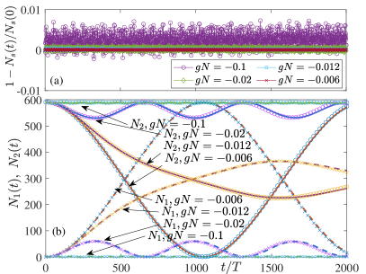
As pointed out in the Introduction, we have previously studied this system with finite interaction using a multi-mode phase-space method, namely the truncated Wigner approximation (TWA) (Wang et al., 2021). Interestingly, we find that for during the whole evolution time only these two Wannier-like modes are occupied. In Fig. 1 (a), we show the total occupation of these two Wannier-like modes , where is the occupation number of the mode . One can see that the fractional change of as a function of time essentially has just small fluctuations around zero. There is also no obvious trend of it increasing during the time window investigated. (In stark contrast, many modes will be occupied if we switch off the driving for the same initial condition and interaction strength - see Ref. (Wang et al., 2021).) The fluctuations shown in this figure reflect the stochastic nature of the TWA calculations (and imply the actual value of might be smaller than the calculation uncertainty). In view of only two modes being important in the TWA calculations for , in this work we apply a so-called two-mode approximation, where we project the Hamiltonian onto the Hilbert sub-space spanned by Fock states based on the two modes and , which we name the stable-island Hilbert space. We emphasize here that, in contrast to fermionic systems that are limited by the Pauli exclusion principle, our bosonic modes can be occupied by an arbitrary number of atoms. Therefore, the two-mode model is a generic many-body problem for large particle number , and the stable-island Hilbert space has a dimension of .
While the two-mode model is described in detail in the next sections, here in Fig. 1 (b), we first show the excellent agreement of the TWA and the two-mode results for different interaction strengths . We emphasize that our TWA calculations Wang et al. (2021) show that a DTC forms for interaction strengths above for an initial state prepared in a harmonic trap with initial position and trap frequency . Quantum fluctuations become significant near this critical interaction strength , and the TWA deviates strongly from the mean-field results. Nevertheless, the two-mode model is still in excellent agreement with the TWA in this case. The TWA in principle can include effects of many (much more than two) modes, and describe the many-body quantum dynamics exactly in the asymptotic limit. On the other hand, although the two-mode model only includes two modes, it can describe the quantum evolution within the truncated stable-island Hilbert space exactly for any arbitary . The excellent agreement between these two models gives us confidence that leakage of atoms to modes other than and is negligible during and most of the atoms seem to be able to remain in the stable-island Hilbert space for a much longer time. The fact that most atoms are “trapped” in this stable-island Hilbert space for a long time breaks the ergodicity of the system and prevents Floquet heating. The underlying physics may be related to a quantum version of the Kolmogorov–Arnold–Moser (KAM) theory as pointed out in Ref. (Sacha, 2020), where the existence of a stable island (as tori in phase space) is robust against weak interactions (Lichtenberg and Lieberman, 1992). However, non-ergodicity in KAM theory can be destroyed by an Arnold diffusion after astronomically long time (Sacha, 2020), implying DTC in our system has a finite lifetime.
III Two-mode approximation
In the two-mode approximation, we assume the bosonic atom field operator can be expanded solely by the two Wannier-like modes
| (5) |
where and are the annihilation and creation operators of a boson in the time-dependent mode . The time-dependence of the creation operators obeys and , which are determined by the properties of , and similar rules apply to the annihilation operators. One can obtain a many-body basis set via the Fock state Dalton et al. (2015)
| (6) |
where is the number of atoms in mode and is the number of atoms in mode . Expanding the many-body state vector in this basis set gives
| (7) |
where the total number of bosonic atoms is a good quantum number and is a suitable frequency (chosen below). These Fock states also satisfy and . We note that, while both the creation/annihilation operators and the Fock-state basis are time-dependent, the matrix elements of any direct product of creation and annihilation operators at the same time are time-independent, e.g., .
The time-evolution of the expansion coefficients is determined by the many-body Schrödinger equation, in a vector form
| (8) |
where is a time-dependent matrix with matrix elements . Here, the effective Hamiltonian operator is given by
| (9) |
where and . The phase factor occurring in the quantum state is given by , where The derivation is given in Appendix A.1. With an understanding that the creation and annihilation operators will always act on the Fock basis and introducing time-independent matrix elements, we hereafter leave implicit the time-dependence of and . The only explicit time-dependence remains in the parameter , which is periodic with period and . The effective Hamiltonian matrix also shares the same periodicity, implying that Eq. (8) can be formally solved using a Floquet approach. A many-body Floquet state and Floquet energy can be defined as
| (10) |
and the time evolution can be obtained via and (see Appendix B). We emphasize here that this approach, namely the many-body Floquet (MBF) approach, is a full and exact many-body quantum calculation as long as only two modes are occupied and depletion to other modes is negligible.
Another time scale in the Hamiltonian is given by which describes the tunneling of a single particle between the two modes. typically is in the order of , much longer than , the period of . An approximation to simplify and understand this problem is therefore to take a high-frequency expansion (HFE) of the Hamiltonian matrix , where , and keep only the lowest order - which is a time-independent effective Hamiltonian matrix. The corresponding Hamiltonian operator of agrees with the one given in Ref. (Sacha, 2015), which can be expressed in the same form as Eq. (9) with replaced by the -average value . However, we note that the time-independent Hamiltonian in Ref. (Sacha, 2015) is derived by expanding and truncating the Floquet Hamiltonian and field operators in an extended space-time Hilbert space. This expansion and truncation is thus an approximation that is effectively equivalent to our HFE approximation. Under the HFE approximation, the time evolution can be approximately given by and the initial condition . Here, and are eigenenergies and eigenstates of : .
Discussions on SDTTSB usually refer to initial states without extensive many-body quantum entanglement, which are physically accessible by simple preparation schemes. As mentioned before, by preparing a BEC in a harmonic trap with suitable potential height and width, the initial condition can be well approximated by a product state . If we turn off the interaction in the preparation stage, the particles can tunnel from to with a tunneling rate , and an additional relative phase can also be induced by some phase-printing scheme. Therefore, in principle, we can prepare a BEC initial product state, which in first quantization is
| (11) |
where all atoms occupy a single mode . Without loss of generality, we choose and .
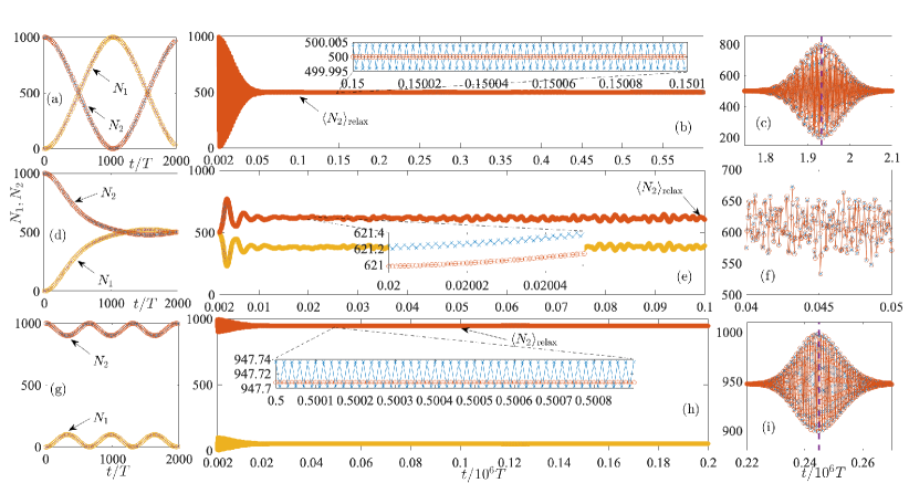
To investigate the dynamical evolution, we study the observables , which play a similar role to the one-body reduced density matrix elements. For simplification of notation, we define . Figure 2 shows a comparison between the MBF approach and HFE approximation for and . The initial state is chosen as wih . Figure 2 (a) (d) and (g) show perfect agreement between the HFE and MBF at relatively short time scales (0 to 2000). At longer time scales , Fig. 2 (b) (e) and (h) show that relaxes to a constant for the HFE. However, for an interaction strength near the critical value , has a relatively larger fluctuation. The MBF results here also show excellent agreement with the HFE, except for an almost negligible oscillation around the that can only be seen in the insets for a large zoom-in scale. This small oscillation can be understood as micro-motion originating from the time-dependence of the many-body Floquet states in the MBF approach. After an even longer evolution time, Fig. 2 (c) and (i) show a strong quantum revival for both strong and weak interaction, but no revival can be seen for the critical case, Fig. 2 (f). We also note that for , the quantum revival seems to be almost perfect, i.e. , in contrast to the case for where . Visible differences between the MBF and HFE show up in the quantum revival regime. Nevertheless, the HFE still accurately predicts the revival time and the overall revival profile. As one can see, the HFE is an excellent approximation. The HFE will also provide an insight into the symmetry breaking and give an analytical explanation of the time-evolution behavior, as shown in the next section.
While the quantum revival is interesting and indicates there is a relatively short transient period of deviation from an almost perfect temporal periodicity, the revival regime is much shorter than the steady-state regime. We discuss the quantum revivals with more detail in Appendix C and focus on the steady-state regime here. We emphasize that this relaxation value of reflects the time-translational symmetry of the steady state. For example, the quantum correlation function (QCF) is given by
| (12) |
where and refer to two different position coordinates. The position probability density at stroboscopic times with can be well approximated by , where the cross-terms can be neglected since and are well separated localized wave-packets at with being integer. We recall that . Therefore, if as in Fig. 2 (b), has the same period as the Hamiltonian, which represents a symmetry-unbroken state. On the other hand, if as in Fig. 2 (h), and , indicating that the system’s state breaks the discrete time-translational symmetry, i.e., a time crystal is present. Figures 2 (h) and (i) predict that the time crystal survives for times out to at least 250,000 driving periods.
We can also define a one-body projection operator (OBP) onto the Gaussian-like localized wave-packet as an observable (Wang et al., 2021). In the first quantization, the OBP is given by , where and lists individual particles as . The expectation value of the OBP can be related to the QCF via . At stroboscopic times with being integer, the OBP can be simplified as
| (13) |
The physical picture is clear: measures how many atoms occupy the Gaussian-like wave-packet at stroboscopic times. When is even [odd], this Gaussian-like wave-packet coincides with []. Therefore, via the investigation of the behavior of , we can obtain the evolution of the observable , which reveals the temporal symmetry of the steady state. If , then implies a -periodicity. On the contrary, if , has -periodicity, indicating SDTTSB. One can define a frequency response observable via the Fourier transformation
| (14) |
where we usually choose and so that is in the steady-state regime. In particular, the sub-harmonic response is given by
| (15) |
where is the population imbalance. (or equivalently ) indicates the symmetry-unbroken phase, and hence can be regarded as an order parameter.
IV Symmetry breaking
Under the HFE approximation, the effective time-independent Hamiltonian satisfies the symmetry determined by the operator which interchanges the mode indices . We find that and . The corresponding effective Hamiltonian operator can be rewritten as
| (16) | ||||
where , , and are the only four distinctive values of constrained by the symmetry (see Appendix A.2). The effective Hamiltonian is invariant under the symmetry operator Here, the number operators are given by , and . One might notice, under a mean-field approximation, that this effective Hamiltonian can be applied to investigate the bosonic self-trapping phenomenon, for example, in a BEC in a double-well potential Albiez et al. (2005). The connection of DTC formation and self-trapping was recognized in Ref. Sacha (2015). Here, we go beyond the mean-field approximation, and numerically investigate the whole eigen spectrum exactly. In our numerical investigation here, we have , , , and . Since the spectrum of is bounded from both below and above, the maximum and minimum eigenenergy of the can be obtained via the mean-field approach in the large limit. Neglecting the term associated with (which is much smaller than , and ), this approach leads to
| (17) |
and
| (18) |
where . (We use the conditions and here. We also focus on the case since is small. See Appendix D for details.) Here, and its physical meaning will be clear below.
For a given total number (since commutes with ), the Hamiltonian can be mapped to the Lipkin–Meshkov–Glick (LMG) model (see Appendix A.3) as (Ribeiro et al., 2008; Mazza and Fabrizio, 2012; Kuroś et al., 2020)
| (19) |
with and which are bosonic spin operators. The LMG Hamiltonian can be applied to describe spin-systems with infinite-range interaction. However, we emphasize here that our system consists of bosonic atoms with zero-range contact interactions. When the two-mode and HFE approximations are applicable, the time-independent LMG Hamiltonian in Eq. (19) becomes an excellent approximation for the Floquet Hamiltonian of the underlying physical system, and determines the dynamical properties of the original system. The LMG Hamiltonian is invariant under the symmetry operator The parameters are given by , . In the case of large and finite , a symmetry-broken edge exists for the LMG Hamiltonian Ribeiro et al. (2008); Mazza and Fabrizio (2012); Russomanno et al. (2017); Kuroś et al. (2020):
| (20) |
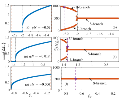
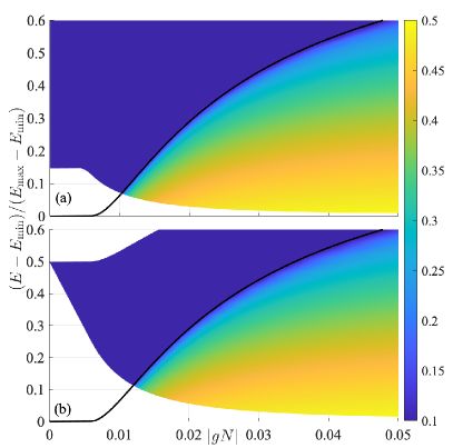
For the eigenenergies are non-degenerate whilst those for are essentially two-fold degenerate (see Fig. 3). From the expression for and , one can observe that for weak interaction , where is defined above and Eq. (73). For strong interaction , and the eigenpairs below and above the edge have distinct features. We emphasise that, according to group representation theory, since is the symmetry group, the eigenstates for would in general be non-degenerate and either even or odd under the symmetry operator, i.e., . However, for , eigenstates that satisfy form near-degenerate pairs and of opposite symmetry, with an energy gap that is exponentially small in . This energy gap is negligible for a large and finite in practice, and becomes exactly zero in the infinite (thermodynamic) limit. Therefore, we can choose a pair of symmetry-broken states that satisfy and , which are given by and . and have the same expectation energies and serve as a degenerate pair of symmetry-broken eigenstates. In contrast, any eigenstates with eigenenergies show no near-degeneracy and these states are symmetry-unbroken. Figures 3 (a), (c) and (e) show the symmetry-breaking edge for , and , respectively. The vertical axis shows the minimum of adjacent gaps: , which is exactly zero if and only if there is a double-degeneracy. One can see that this quantity indeed becomes essentially zero at , which is denoted by the black vertical dash-dotted lines. The red dashed line on the right (left) indicates (). For , only a symmetry-unbroken phase exists, since , and no near-degenerate pairs of energy levels occur.
A particularly useful observable to illustrate the importance of the symmetry-breaking edge is and , where and
| (21) |
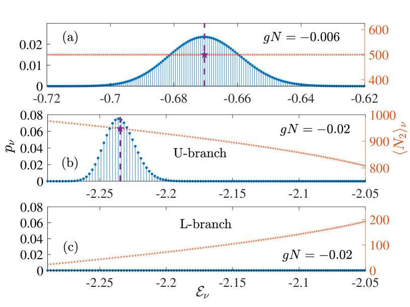
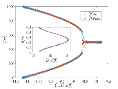
For symmetry-unbroken states, the permutation symmetry between modes ensures that . On the other hand, for symmetry-broken states, we have and , but in general . Without loss of generality, we denote (hence the U- and L-branch). Figures 3 (b), (d) and (f) show as a function of , with initial state and . The black dash-dotted vertical line indicates the symmetry-broken edge, which illustrates the onset of bifurcation of as a function of . We also show by the purple pentagram symbol and the initial energy by the dashed vertical line. Numerically, is calculated by averaging over a time-window of driving periods at . We can see that the relaxation value lies on the curve of the corresponding branches, which can be understood via dephasing. In general, for an initial state , the time-evolution of an observable is given by . Typically, only has noticeable values around a small energy window close to the initial energy. If there is no degeneracy, after long enough time, dephasing leads to , where is sometimes called the diagonal ensemble, and is the projection probability of the initial state to the ’s eigenstate. Essentially, the contributions for cancel out for large , as the phase factors in become more random. The initial energy can also be given by the diagonal ensemble . When the initial energy is well above the broken edge, gives as shown in Fig. 4 (a). When the initial energy is below the broken edge, as shown in Fig. 4 (b) and (c), we find that for initial state , only the U-branch has noticeable projections, since the degeneracy is lifted in a single branch, the dephasing formula still works, and gives .
To further explore the corresponding relation between the initial energy and the relaxation value, we investigate the case with an initial state defined in Eq. (11) with all bosons in a mode given by which has initial energy . Since this initial state represents all atoms occupying the same single-particle state, the initial energy reduces to a mean-field expression
| (22) | ||||
Figure 5 shows as a function of the initial energy for different initial states , and as a function of for . As one can see, in the deep regime in all branches (L, U and S), these two curves overlap, implying the dephasing mechanism leads to relaxation except very close to the critical point where finite-size effects become important. The inset shows the corresponding relationship between the initial state and the initial energy . We also note that the initial states considered here are initial states with no multi-mode entanglement, as these are the initial states of interest for spontaneous symmetry-breaking physics.
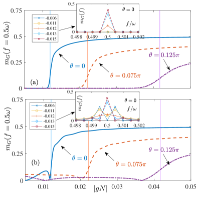
In Fig. 6 (a), we investigate the subharmonic response of the steady state as a function of for different initial states , which changes from to a finite value abruptly around a critical indicated by the thin vertical lines. These critical values for different can be obtained by equating and as shown in Fig. 7 (a). The inset of Fig. 6 (a) shows the frequency response for close to and the initial state . We can see that a single sharp peak appears abruptly when . However, in realistic experiments, one might not be able to access such very long evolution times. In Fig. 6 (b), we show that the transient behavior at relatively short times can be regarded as a precurser. One can see that, while not as smooth and clean as Fig. 6 (a), still shows an abrupt change to a much larger value near . In the inset, one can see that the frequency response of the transient states for at short times shows a double-peak structure for and which changes to a single-peak structure for , the same as the observation in (Wang et al., 2021). In the steady-state regime, we now have the intriguing situation where, as the magnitude of the interaction is increased from that just below the critical interaction to just above , the period of the bouncing atom cloud changes from period to period , to form a DTC. Although the numerical results presented here are calculated for a finite , we believe the conclusions remain valid in the thermodynamic limit ( and finite ). An analysis of the finite size effect is given in Appendix E.
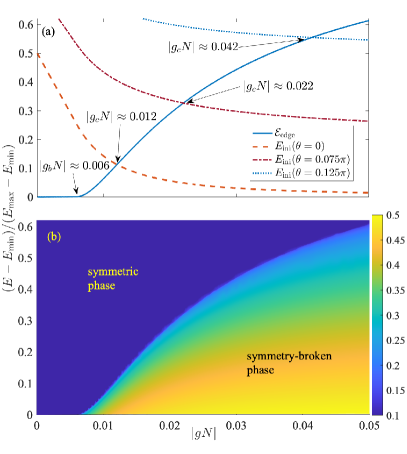
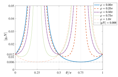
The whole phase diagram for different initial energy and interaction strength is summarized in Fig. 7. The solid line in Fig. 7 (a) shows the normalized , which agrees with the phase boundary indicated by the subharmonic response in Fig. 7 (b). The dashed, dash-dotted and dotted curves in Fig. 7 (a) show the initial energy as a function of for different initial states defined in Eq. (11) with and , respectively. The initial energy curve crosses the edge at the critical shown in Fig. 6. For a general initial product state , the critical as a function of for a given is shown in Fig. 8. (See Appendix D for details.) This shows that the onset of DTC formation depends on the choice of initial state through the initial energy , as well as on the system parameters , . Here, the critical for the onset of DTC formation is determined by equating the initial energy with the .
These phase diagrams indicate that the symmetry of the steady state characterized by the subharmonic response is determined by whether the initial energy is above or below the symmetry-breaking edge of the eigenenergy spectrum for a given interaction strength . The symmetry-breaking edge thus gives the abrupt phase transition boundary. This phase transition boundary is valid for any general initial product states (see Appendix D for details).
This symmetry breaking is associated with the time-translational symmetry breaking in the time crystal. Denoting the elements of the eigenstate vector as , the eigenstates can be written as . The permutation operator transforms the eigenstates as
| (23) | ||||
For symmetry-unbroken eigenstates, we also have , which leads to . Therefore, these eigenstates are -periodic, and satisfy the same discrete time-translational symmetry as the Hamiltonian. In contrast, for a pair of symmetry-broken approximate eigenstates, we have . These eigenstates therefore have a period of instead of , which breaks the discrete time-translational symmetry of the Hamiltonian. The eigenstates of can be regarded as an approximation of the many-body Floquet states in Eq. (9) with period . Therefore, the near-degeneracy of and in the symmetry-breaking regime plays the same role as the nearly -pairing of -Floquet states in MBL and many-body quantum scar DTCs (Sacha, 2020).
V Summary
We have derived a two-mode model from standard quantum field theory to study discrete time-translational symmetry breaking and the formation of DTCs in a Bose-Einstein condensate bouncing resonantly on an oscillating mirror. The validity of this simple many-body model has been investigated by comparing with previous multimode phase-space many-body calculations based on the TWA approach (Wang et al., 2021). The greatly reduced computational times using this simple many-body model allows us to study the long-time dynamical evolution of the many-body system. Using two Wannier modes constructed from two single-particle Floquet states, the dynamical evolution has been studied both via a fully time-dependent Floquet Hamiltonian (MBF) and by using a time-independent Hamiltonian based on a high frequency expansion (HFE). In the HFE approach, the Hamiltonian is equivalent to the Lipkin-Meshkov-Glick model (Ribeiro et al., 2008; Mazza and Fabrizio, 2012; Kuroś et al., 2020). The main initial state chosen has all bosons in the Wannier mode that closely resembles the condensate mode for a BEC in a harmonic trap treated in our TWA approach. However, a wide variety of initial states based on the two Wannier modes has also been studied. A new criterion for demonstrating the periodicity at stroboscopic times has been developed which involves the mean number of bosons in each Wannier mode.
We find that the evolution investigated in previous studies in the time-window out to about 2000 driving periods actually involves “short-time” transient phenomena though DTC formation is still shown if the inter-boson interaction is strong enough. The two-mode compares well with the TWA approach in regard to the critical for DTC formation. However the TWA treatment is needed to verify that quantum depletion to other modes is negligible. After much longer evolution times, initial states with no long-range correlations relax to a steady state and eventually show short-lived quantum revivals. In the steady state the mean boson number in each Wannier mode demonstrates that stroboscopic DTC behavior occurs for the same interaction regime found in the previous TWA calculations, the critical value for DTC formation with periodicity being about for the parameters considered and the initial state , which is the easiest to prepare in an experiment. However, the two-mode theory now more clearly shows that in the steady-state regime, for the initial state and for smaller , only periodicity occurs.
For a general initial product state condition , the magnitude of the critical value can be as low as (see Fig. 8 and Appendix D). The long-time behavior can be understood via the many-body Floquet quasi-eigenenergy spectrum of the two-mode model. For sufficiently strong interaction, a symmetry-breaking edge appears in the spectrum, where all quasi-eigenstates below the edge are symmetry-breaking while those above the edge are symmetric. The position of the edge is found to depend on the boson number and the inter-mode tunnelling rate, and gives as a function of without explicit dependence on initial details . Finally, a phase diagram showing regions of symmetry-broken and symmetric phases for differing initial energies and interaction strengths summarises the subharmonic response results. Here, we now allow for initial states where all bosons occupy a mode which is a linear combination of the two Wannier modes parameterized by . Our results predict that in the steady-state regime, after about driving periods (for the parameters considered), as the magnitude of the interaction is increased from just below to just above the critical interaction strength the period of the bouncing atom cloud changes abruptly from the driving period to period , to form a discrete time crystal. The present two-mode theory approach predicts that the discrete time crystal survives for times out to 250,000 driving periods. However, after astronomically long time, the escape of atoms to other modes beyond our two-mode model might eventually occur, leading to a finite lifetime of our long-lived DTC.
VI ACKNOWLEDGEMENTS
J.W acknowledges support from an ARC DECRA Grant no. DE180100592). The project is supported by an ARC Discovery Project grant (Grant no. DP190100815). K.S. acknowledges support of the National Science Centre Poland via Project 2018/31/B/ST2/00349.
Appendix A Derivations
In this Appendix we derive some of the key equations used in the main body of the paper.
A.1 Derivation of Equations (8), (9)
Substituting the two-mode expansion Eq. (5) of the field operators into the Hamiltonian in Eq. (1) gives
| (24) |
where
| (25) |
| (26) |
Using Eq. (4) for the Wannier modes and Eq. (3) for the Floquet modes we then find that
| (27) |
where
| (28) |
| (29) |
| (30) |
Hence the Hamiltonian is given by
| (31) |
We now expand the quantum state as
| (32) |
where are Fock states given by Eq. (6), with , bosonic atoms in modes , , respectively. Note that these basis states are time-dependent, as are the amplitudes .
Substituting into the time-dependent Schrödinger equation then gives
| (33) | ||||
so taking the scalar product with on each side gives
| (34) | ||||
We can eliminate the terms by using the expansion for the time-independent field creation operator to first derive an equation for the time derivative of the Wannier mode creation operators
| (35) | ||||
Hence the time derivative of the basis states is
| (36) | ||||
where we have used the result that the commute with any .
Hence on substituting for in Eq. (34) we see that the terms cancel out leaving
| (37) |
If we write we then find that the terms involving cancel out leaving
| (38) |
so we now have
| (39) |
| (40) |
where
| (41) |
and the quantum state is now given by
| (42) |
The phase factor is not physically important. Thus, Eqs. (40), (41) are equivalent to Eqs. (7), (8) in the main part of the paper after introducing the matrix for and a column vector for the amplitudes via and .
A.2 Derivation of Equation (16)
At this stage the HFE approximation has been made, so that is replaced by given by
| (43) |
| (44) |
which now means that all the coefficients in are time-independent.
Many of the coefficients are inter-related. Firstly, from the definition of we see that
| (45) |
which leads to
| (46) |
In addition to these coefficients, there are more, namely , , and .
We can show more inter-relationships by expressing the Wannier states by introducing the notation and for Wannier mode and for Wannier mode . Thus , where . We can then divide the time interval to in the definition for into time intervals to and to , and then make use of the properties and to convert the integral from to back into an integral from to . This gives the following expression for
| (47) | ||||
where the , dependence of the functions is left understood. This enables us to establish more inter-relationships, as the second term for one is often the first term for another , and vice-versa. Hence we find that
| (48) |
| (50) |
since we can show that
| (51) |
is real.
Also, we have
| (52) |
which are all real.
Hence, overall we have only independent coefficients which can be listed as
| (53) | ||||
This obviously enables the expression for to be simplified. Hence we have
| (54) | ||||
which is the same as Eq. (16).
A.3 Derivation of Lipkin-Meshkov-Glick Hamiltonian - Equation (19)
Here, we recast in terms of bosonic spin operators defined as
| (55) |
which along with and the standard bosonic commutation rules for the mode annihilation, creation operators enable the following substitutions to be made within
| (56) | ||||
From Eq. (54) we have
| (57) | ||||
so as we are only dealing with states which are eigenstates for the total boson number, we can replace by .
After combining similar terms we get
| (58) | ||||
which can be written as
| (59) |
where
| (60) | ||||
This is the same as Eq (19) in the main body of the paper, if the small term involving is discarded.
Appendix B Many-Body Floquet mode solution
We can define many-body Floquet states and Floquet energies as the solutions of the matrix equations (Eq. (10))
| (61) |
It can then be confirmed that a solution for the amplitudes can be found in the form
| (62) |
where the are time-independent.
Appendix C Quantum revival
The quantum revival time can be obtained from the spectrum (Buchleitner et al., 2002; Dalton and Ghanbari, 2012)
| (64) |
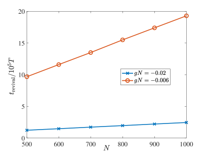
where are understood to be taken from the same branch (so that there is no near-degeneracy), and is the index for ascending eigenenergies. indicates the closest to the initial energy , and the second derivative can be approximated by . Interestingly, we numerically find that the revival time linearly depends on the particle number , as shown in Fig. 9. In other words, in the infinite limit, the revival would not be accessible.
Appendix D Initial product states
For initial states with and given by Eq. (11), all atoms occupy the same mode , and hence the energy can be given by a mean-field approach in the large limit, i.e., by replacing the creation and annhilation operators in the Hamiltonian (16) via
| (65) |
Neglecting the small terms associated with , the energy functional is given by
| (66) |
where . Inserting the definitions of and given in the main text
| (67) |
and
| (68) |
leads to
| (69) | ||||
which agrees with Eq. (22) in the main text. Equating [given in Eq. (22) or Eq. (69)] with the broken symmetry edge [given in Eq. (20)] leads to the critical interaction strength as a function of for a given
| (70) |
which is shown in Fig. 8. It is also important to note that the phase diagram does not depend explicitly on , where the subharmonic response is essentially zero (nonzero) for () for a given Figures 7 (b), 10 (a) and (b) show for different initial states , and , respectively, which agree with each other. However, the condition would limit the range of that can be accessed, which is indicated by the white areas (no data) in Figs. 10 (a) and (b).
In the large limit, since the spectrum is bounded from both below and above, the minimum and maximum energy state should also be well approximated by the mean-field expression, i.e., and . These expressions are explicitly given by
| (71) |
and for the negative considered in this work
| (72) |
whose expression in the second line can also be explicitly written as . In this work, we focus on the case , therefore; the critical condition gives
| (73) |
One can notice that the initial state corresponding to actually corresponds to the “Wannier initial condition” in our previous study (Wang et al., 2021). We also find here that the minimum value of for DTC formation based on Wannier initial conditions is given by . This corresponds to in Fig. 7 (b).
Appendix E Finite size effect
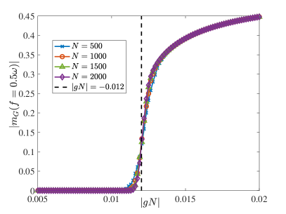
In Ref. (Pizzi et al., 2020), it is noticed that the amplitude of the subharmonic response of a DTC in a many-body quantum scar system is exponentially suppressed with system size, and in principle would disappear in the thermodynamic limit. In contrast, the subharmonic response of a DTC in a MBL system does not decay with respect to system size. It is thus interesting to study the finite size effect of our system, whose eigenspectra are different from both many-body quantum scar and MBL systems. Figure 11 shows the subharmonic response as a function of for different . We observe that the subharmonic response in the symmetry-broken phase does not decay with respect to , similar to the DTC in MBL systems.
References
- Wilczek (2012) Frank Wilczek, “Quantum time crystals,” Phys. Rev. Lett. 109, 160401 (2012).
- Watanabe and Oshikawa (2015) Haruki Watanabe and Masaki Oshikawa, “Absence of quantum time crystals,” Phys. Rev. Lett. 114, 251603 (2015).
- Kozin and Kyriienko (2019) Valerii K. Kozin and Oleksandr Kyriienko, “Quantum time crystals from Hamiltonians with long-range interactions,” Phys. Rev. Lett. 123, 210602 (2019).
- Sacha (2015) Krzysztof Sacha, “Modeling spontaneous breaking of time-translation symmetry,” Phys. Rev. A 91, 033617 (2015).
- Khemani et al. (2016) Vedika Khemani, Achilleas Lazarides, Roderich Moessner, and S. L. Sondhi, “Phase structure of driven quantum systems,” Phys. Rev. Lett. 116, 250401 (2016).
- Else et al. (2016) Dominic V. Else, Bela Bauer, and Chetan Nayak, “Floquet time crystals,” Phys. Rev. Lett. 117, 090402 (2016).
- Yao et al. (2017) N. Y. Yao, A. C. Potter, I.-D. Potirniche, and A. Vishwanath, “Discrete time crystals: Rigidity, criticality, and realizations,” Phys. Rev. Lett. 118, 030401 (2017).
- Zhang et al. (2017) J. Zhang, P. W. Hess, A. Kyprianidis, P. Becker, A. Lee, J. Smith, G. Pagano, I.-D. Potirniche, A. C. Potter, A. Vishwanath, N. Y. Yao, and C. Monroe, “Observation of a discrete time crystal,” Nature 543, 217 (2017).
- Choi et al. (2017) Soonwon Choi, Joonhee Choi, Renate Landig, Georg Kucsko, Hengyun Zhou, Junichi Isoya, Fedor Jelezko, Shinobu Onoda, Hitoshi Sumiya, Vedika Khemani, Curt von Keyserlingk, Norman Y. Yao, Eugene Demler, and Mikhail D. Lukin, “Observation of a discrete time crystal,” Nature 543, 221 (2017).
- Rovny et al. (2018a) Jared Rovny, Robert L. Blum, and Sean E. Barrett, “Observation of discrete-time-crystal signatures in an ordered dipolar many-body system,” Phys. Rev. Lett. 120, 180603 (2018a).
- Pal et al. (2018) Soham Pal, Naveen Nishad, T. S. Mahesh, and G. J. Sreejith, “Temporal order in periodically driven spins in star-shaped clusters,” Phys. Rev. Lett. 120, 180602 (2018).
- Rovny et al. (2018b) Jared Rovny, Robert L. Blum, and Sean E. Barrett, “ NMR study of discrete time-crystalline signatures in an ordered crystal of ammonium dihydrogen phosphate,” Phys. Rev. B 97, 184301 (2018b).
- Smits et al. (2018) J. Smits, L. Liao, H. T. C. Stoof, and P. van der Straten, “Observation of a space-time crystal in a superfluid quantum gas,” Phys. Rev. Lett. 121, 185301 (2018).
- Liao et al. (2019) L. Liao, J. Smits, P. van der Straten, and H. T. C. Stoof, “Dynamics of a space-time crystal in an atomic bose-einstein condensate,” Phys. Rev. A 99, 013625 (2019).
- Smits et al. (2020) J. Smits, H. T. C. Stoof, and P. van der Straten, “On the long-term stability of space-time crystals,” New J. Phys. 22, 105001 (2020).
- Else et al. (2017) Dominic V. Else, Bela Bauer, and Chetan Nayak, “Prethermal phases of matter protected by time-translation symmetry,” Phys. Rev. X 7, 011026 (2017).
- Russomanno et al. (2017) Angelo Russomanno, Fernando Iemini, Marcello Dalmonte, and Rosario Fazio, “Floquet time crystal in the lipkin-meshkov-glick model,” Phys. Rev. B 95, 214307 (2017).
- Matus and Sacha (2019) Paweł Matus and Krzysztof Sacha, “Fractional time crystals,” Phys. Rev. A 99, 033626 (2019).
- Zhu et al. (2019) Bihui Zhu, Jamir Marino, Norman Y Yao, Mikhail D Lukin, and Eugene A Demler, “Dicke time crystals in driven-dissipative quantum many-body systems,” New J. Phys. 21, 073028 (2019).
- Sun et al. (2019) Feng-Xiao Sun, Qiongyi He, Qihuang Gong, Run Yan Teh, Margaret D Reid, and Peter D Drummond, “Discrete time symmetry breaking in quantum circuits: exact solutions and tunneling,” New J. Phys. 21, 093035 (2019).
- Machado et al. (2020) Francisco Machado, Dominic V. Else, Gregory D. Kahanamoku-Meyer, Chetan Nayak, and Norman Y. Yao, “Long-range prethermal phases of nonequilibrium matter,” Phys. Rev. X 10, 011043 (2020).
- Natsheh et al. (2021) Muath Natsheh, Andrea Gambassi, and Aditi Mitra, “Critical properties of the Floquet time crystal within the Gaussian approximation,” Phys. Rev. B 103, 014305 (2021).
- Pizzi et al. (2021) Andrea Pizzi, Johannes Knolle, and Andreas Nunnenkamp, “Higher-order and fractional discrete time crystals in clean long-range interacting systems,” Nat. Comm. 12, 2341 (2021).
- Sacha and Zakrzewski (2018) Krzysztof Sacha and Jakob Zakrzewski, “Time crystals: a review,” Rep. Prog. Phys. 81, 016401 (2018).
- Khemani et al. (2019) Vedika Khemani, Roderich Moessner, and S. L. Sondhi, “A brief history of time crystals,” (2019), arXiv: 1910.10745.
- Else et al. (2020) Dominic V. Else, Christopher Monroe, Chetan Nayak, and Norman Yao, “Discrete time crystals,” Ann. Rev. Cond. Matt. Phys. 11, 467 (2020).
- Sacha (2020) Krzysztof Sacha, Time Crystals (Springer, 2020).
- D’Alessio and Rigol (2014) Luca D’Alessio and Marcos Rigol, “Long-time behavior of isolated periodically driven interacting lattice systems,” Phys. Rev. X 4, 041048 (2014).
- Lazarides et al. (2014) Achilleas Lazarides, Arnab Das, and Roderich Moessner, “Equilibrium states of generic quantum systems subject to periodic driving,” Phys. Rev. E 90, 012110 (2014).
- Ponte et al. (2015a) Pedro Ponte, Anushya Chandrana, Z. Papić, and Dmitry A. Abanin, “Periodically driven ergodic and many-body localized quantum systems,” Ann. Phys. 353, 196 (2015a).
- Ponte et al. (2015b) Pedro Ponte, Z. Papić, Fran çois Huveneers, and Dmitry A. Abanin, “Many-body localization in periodically driven systems,” Phys. Rev. Lett. 114, 140401 (2015b).
- Lazarides et al. (2015) Achilleas Lazarides, Arnab Das, and Roderich Moessner, “Fate of many-body localization under periodic driving,” Phys. Rev. Lett. 115, 030402 (2015).
- Abanin et al. (2016) Dmitry Abanin, Wojciech De Roeck, and François Huveneers, “A theory of many-body localization in periodically driven systems,” Ann. Phys. 372, 1–11 (2016).
- Kuwahara et al. (2016) Tomotaka Kuwahara, Takashi Mori, and Keiji Saito, “Floquet-Magnus theory and generic transient dynamics in periodically driven many-body quantum systems,” Ann. Phys. 367, 96 (2016).
- Canovi et al. (2016) Elena Canovi, Marcus Kollar, and Martin Eckstein, “Stroboscopic prethermalization in weakly interacting periodically driven systems,” Phys. Rev. E 93, 012130 (2016).
- Machado et al. (2019) Francisco Machado, Gregory D. Kahanamoku-Meyer, Dominic V. Else, Chetan Nayak, and Norman Y. Yao, “Exponentially slow heating in short and long-range interacting Floquet systems,” Phys. Rev. Research 1, 033202 (2019).
- Turner et al. (2018) C. J. Turner, A. A. Michailidis, D. A. Abanin, M. Serbyn, and Z. Papić, “Weak ergodicity breaking from quantum many-body scars,” Nat. Phys. 14, 745 (2018).
- Michailidis et al. (2020) A. A. Michailidis, C. J. Turner, Z. Papić, D. A. Abanin, and M. Serbyn, “Slow quantum thermalization and many-body revivals from mixed phase space,” Phys. Rev. X 10, 011055 (2020).
- Surace et al. (2021) Federica Maria Surace, Matteo Votto, Eduardo Gonzalez Lazo, Alessandro Silva, Marcello Dalmonte, and Giuliano Giudici, “Exact many-body scars and their stability in constrained quantum chains,” Phys. Rev. B 103, 104302 (2021).
- Pizzi et al. (2020) Andrea Pizzi, Daniel Malz, Giuseppe De Tomasi, Johannes Knolle, and Andreas Nunnenkamp, “Time crystallinity and finite-size effects in clean Floquet systems,” Phys. Rev. B 102, 214207 (2020).
- Shirley (1965) Jon H. Shirley, “Solution of the Schrödinger equation with a Hamiltonian periodic in time,” Phys. Rev. 138, B979–B987 (1965).
- Sambe (1973) Hideo Sambe, “Steady states and quasienergies of a quantum-mechanical system in an oscillating field,” Phys. Rev. A 7, 2203–2213 (1973).
- Eckardt and Anisimovas (2015) André Eckardt and Egidijus Anisimovas, “High-frequency approximation for periodically driven quantum systems from a Floquet-space perspective,” New J. Phys. 17, 093039 (2015).
- von Keyserlingk et al. (2016) C. W. von Keyserlingk, Vedika Khemani, and S. L. Sondhi, “Absolute stability and spatiotemporal long-range order in Floquet systems,” Phys. Rev. B 94, 085112 (2016).
- von Keyserlingk and Sondhi (2016) C. W. von Keyserlingk and S. L. Sondhi, “Phase structure of one-dimensional interacting Floquet systems. ii. symmetry-broken phases,” Phys. Rev. B 93, 245146 (2016).
- Moessner and Sondhi (2017) R. Moessner and S. L. Sondhi, “Equilibration and order in quantum Floquet matter,” Nat. Phys. 13, 424 (2017).
- Giergiel et al. (2018) Krzysztof Giergiel, Arkadiusz Kosior, Peter Hannaford, and Krzysztof Sacha, “Time crystals: Analysis of experimental conditions,” Phys. Rev. A 98, 013613 (2018).
- Giergiel et al. (2020) Krzysztof Giergiel, Tien Tran, Ali Zaheer, Arpana Singh, Andrei Sidorov, Krzysztof Sacha, and Peter Hannaford, “Creating big time crystals with ultracold atoms,” New J. Phys. 22, 085004 (2020).
- Kuroś et al. (2020) Arkadiusz Kuroś, Rick Mukherjee, Weronika Golletz, Frederic Sauvage, Krzysztof Giergiel, Florian Mintert, and Krzysztof Sacha, “Phase diagram and optimal control for n-tupling discrete time crystal,” New J. Phys. 22, 095001 (2020).
- Wang et al. (2021) Jia Wang, Peter Hannaford, and Bryan J Dalton, “Many-body effects and quantum fluctuations for discrete time crystals in Bose-Einstein condensates,” New J. Phys. , 063012 (2021).
- Albiez et al. (2005) Michael Albiez, Rudolf Gati, Jonas Fölling, Stefan Hunsmann, Matteo Cristiani, and Markus K. Oberthaler, “Direct observation of tunneling and nonlinear self-trapping in a single bosonic Josephson junction,” Phys. Rev. Lett. 95, 010402 (2005).
- Buchleitner et al. (2002) Andreas Buchleitner, Dominique Delande, and Jakub Zakrzewski, “Non-dispersive wave packets in periodically driven quantum systems,” Phys. Rep. 368, 409 (2002).
- Lichtenberg and Lieberman (1992) A. J. Lichtenberg and M.A. Lieberman, Regular and Chaotic Dynamics (Springer, 1992).
- Dalton et al. (2015) B J Dalton, J Jeffers, and S M Barnett, Phase Space Methods for Degenerate Quantum Gases (Oxford: Oxford University Press, 2015).
- Ribeiro et al. (2008) Pedro Ribeiro, Julien Vidal, and Rémy Mosseri, “Exact spectrum of the Lipkin-Meshkov-Glick model in the thermodynamic limit and finite-size corrections,” Phys. Rev. E 78, 021106 (2008).
- Mazza and Fabrizio (2012) Giacomo Mazza and Michele Fabrizio, “Dynamical quantum phase transitions and broken-symmetry edges in the many-body eigenvalue spectrum,” Phys. Rev. B 86, 184303 (2012).
- Dalton and Ghanbari (2012) B.J. Dalton and S. Ghanbari, “Two mode theory of Bose-Einstein condensates: interferometry and the Josephson model,” J. Mod. Opt. 59, 287 (2012).