Discrete-Time Distributed Observers over Jointly Connected Switching Networks and an Application

Tao Liu and Jie Huang This work has been supported by the Research Grants Council of the Hong Kong Special Administration Region under grant No. 14200617. (Corresponding author: Jie Huang.)Tao Liu and Jie Huang are with the Department of Mechanical and Automation Engineering, The Chinese University of Hong Kong, Shatin, N.T., Hong Kong. E-mail: tliu2@mae.cuhk.edu.hk, jhuang@mae.cuhk.edu.hk

Abstract

In this paper, we first establish an exponential stability result for a class of linear switched systems and then apply this result to show the existence of the distributed observer for a discrete-time leader system over jointly connected switching networks. A special case of this result leads to the solution of a leader-following consensus problem of multiple discrete-time double-integrator systems over jointly connected switching networks. Then, we further develop the adaptive distributed observer for the discrete-time leader system over jointly connected switching networks, which has the advantage over the distributed observer in that it does not require that every follower know the system matrix of the leader system. As an application of the discrete-time distributed observer, we will solve the cooperative output regulation problem of a discrete-time linear multi-agent system over jointly connected switching networks. A leader-following formation problem of mobile robots will be used to illustrate our design. This problem cannot be handled by any existing approach.

I Introduction

The distributed observer for a leader system is a distributed dynamic compensator that can estimate the state of the leader distributively in a sense to be described in Section III. It is an effective tool in dealing with various cooperative control problems for multi-agent systems. For a linear continuous-time leader system of the following form:

\dot{v}(t)=Sv(t),\qquad t\geq 0

(1)

where $v\in\mathbb{R}^{q}$ and $S\in\mathbb{R}^{q\times q}$ is a constant system matrix, a distributed observer was first developed in [17] over connected static networks, and then in [18] over jointly connected switching networks. On the other hand, for a linear discrete-time leader system of the following form:

v(t+1)=Sv(t),\qquad t=0,1,2,\ldots,

(2)

a distributed observer was also developed in [19] over connected static networks, and then in [20] over jointly connected switching networks.

It was shown in [18] that a distributed observer for (1) over jointly connected switching networks always exists if all the eigenvalues of the matrix $S$ have zero or negative real parts. However, the existence conditions of a distributed observer for (2) over jointly connected switching networks are much more stringent than the continuous-time case. Specifically, the result in [20] further requires that some subgraph of the jointly connected switching digraph be undirected and the matrix $S$ be marginally stable in the sense that all the eigenvalues of $S$ on the unit circle must be semi-simple. Moreover, while the solution of each subsystem of the distributed observer for (1) converges to the state of (1) exponentially, the solution of each subsystem of the discrete-time distributed observer for (2) is only shown to converge to the state of (2) asymptotically.

Due to this significant gap between the result of the distributed observer for the continuous-time system (1) and the result of the distributed observer for the discrete-time system (2), the applications of discrete-time multi-agent control systems also lag far behind the applications of continuous-time multi-agent control systems. For example, while the leader-following consensus problem of multiple continuous-time double-integrator systems over jointly connected switching networks was solved as early as 2012 in [18], the leader-following consensus problem of multiple discrete-time double-integrator systems over jointly connected switching networks is yet to be studied.

In this paper, we will further study the distributed observer for the discrete-time system (2) over jointly connected switching networks. We first establish an exponential stability result for a class of linear switched systems and then apply this result to show the existence of the distributed observer for the discrete-time system (2) over jointly connected switching networks. A special case of this result leads to the solution of the leader-following consensus problem of multiple discrete-time double-integrator systems over jointly connected switching networks. Then, we further develop the adaptive distributed observer for the discrete-time system (2) over jointly connected switching networks. It is noted that the adaptive distributed observer for the continuous-time system (1) was proposed in [1] over jointly connected switching networks. An advantage of the adaptive distributed observer over the distributed observer is that, it does not require that every follower know the system matrix $S$ of the leader. The discrete-time version of the adaptive distributed observer over connected static networks was proposed in [8] and further improved in [11]. However, the discrete-time version of the adaptive distributed observer over jointly connected switching networks is still missing. As an application of the discrete-time distributed observer, we will solve the cooperative output regulation problem of a discrete-time linear multi-agent system over jointly connected switching networks. A leader-following formation problem of mobile robots will be used to illustrate our design. This problem cannot be handled by any existing approach.

The rest of the paper is organized as follows. We present some technical lemmas in Section II and then establish the distributed observer and the adaptive distributed observer in Section III. In Section IV, we show the solvability of the cooperative output regulation problem of a discrete-time linear multi-agent system over jointly connected switching networks via the distributed observer approach. An example is given in Section V and the paper is concluded in Section VI with some remarks.

Notation. $\mathbb{Z}^{+}$ denotes the set of all nonnegative integers. Let $x:\mathbb{Z}^{+}\rightarrow\mathbb{R}^{n}$ . Then, we often denote $x(t)$ , $t\in\mathbb{Z^{+}}$ by a shorthand notation $x$ where no confusion occurs. $\rho(A)$ denotes the spectral radius, i.e., the maximal magnitude of the eigenvalues of a real square matrix $A$ . $\bm{1}_{N}$ denotes an $N$ dimensional column vector whose components are all $1$ . $\otimes$ denotes the Kronecker product of matrices. $||x||$ denotes the Euclidean norm of a vector $x$ and $\|A\|$ denotes the induced Euclidean norm of a real matrix $A$ . For $X_{i}\in\mathbb{R}^{n_{i}\times q}$ , $i=1,\dots,m$ , $\text{col}(X_{1},\dots,X_{m})=\left[\begin{array}[]{ccc}X_{1}^{T}&\cdots&X_{m}^{T}\\ \end{array}\right]^{T}.$

II Some Technical Lemmas

In what follows, we use $\bar{\mathcal{G}}_{\sigma(t)}=\left(\bar{\mathcal{V}},\bar{\mathcal{E}}_{\sigma(t)}\right)$ to denote a switching digraph¹¹1See Appendix for a summary of notation on digraph. with $\bar{\mathcal{V}}=\{0,1,\ldots,N\}$ and $\sigma:\mathbb{Z}^{+}\mapsto\mathcal{P}=\{1,2,\dots,n_{0}\}$ . This digraph is said to be jointly connected if there exists $T\geq 0$ such that, for all $t\in\mathbb{Z}^{+}$ , every node $i,i=1,\ldots,N$ , is reachable from the node $0$ in the union digraph $\bigcup_{s=0}^{T}\bar{\mathcal{G}}_{\sigma(t+s)}$ .

Let us first list the following two assumptions.

Assumption 1

The digraph $\bar{\mathcal{G}}_{\sigma(t)}$ is jointly connected.

Assumption 2

$\rho(S)\leq 1$ .

Denote the weighted adjacency matrix of $\bar{\mathcal{G}}_{\sigma(t)}$ by $\bar{\mathcal{A}}_{\sigma(t)}=[a_{ij}(t)]_{i,j=0}^{N}\in\mathbb{R}^{(N+1)\times(N+1)}$ . Since $\mathcal{P}$ only contains finitely many elements, there exist real numbers $e_{\max}\geq e_{\min}>0$ such that $e_{\min}\leq a_{ij}(t)\leq e_{\max}$ for all $t\in\mathbb{Z}^{+}$ and $(j,i)\in\bar{\mathcal{E}}_{\sigma(t)}$ .

For $i,j=0,1,\ldots,N$ , let

\omega_{ij}(t)=\begin{cases}\frac{1}{1+\sum_{j=0}^{N}a_{ij}(t)},\quad&\text{if}\ i=j\\ \frac{a_{ij}(t)}{1+\sum_{j=0}^{N}a_{ij}(t)},\quad&\text{otherwise.}\end{cases}

Then, we call $\bar{\Omega}_{\sigma(t)}=[\omega_{ij}(t)]_{i,j=0}^{N}\in\mathbb{R}^{(N+1)\times(N+1)}$ as the normalized weighted adjacency matrix of $\bar{\mathcal{G}}_{\sigma(t)}$ .

Now consider the following linear switched system:

x(t+1)=\bar{\Omega}_{\sigma(t)}x(t),\qquad t\geq t_{0}\geq 0

(3)

where $x=\text{col}(x_{0},x_{1},\ldots,x_{N})$ , $x_{i}\in\mathbb{R},i=0,1,\ldots,N$ .

The following proposition is extracted from Proposition 1 in [12].

Proposition 1

Under Assumption 1, for any $x(t_{0})$ , the $(N+1)$ components of the solution $x(t)$ of system (3) converge uniformly to a common value as $t\to\infty$ . $\Box$

Remark 1

Let $\hat{\mathcal{G}}_{\sigma(t)}$ be a subgraph of $\bar{\mathcal{G}}_{\sigma(t)}$ , which is obtained from $\bar{\mathcal{G}}_{\sigma(t)}$ by removing all edges $(i,0)$ for all $i=1,\ldots,N$ . Then, Assumption 1 implies that $\hat{\mathcal{G}}_{\sigma(t)}$ is also jointly connected.

Now let $\Lambda_{\sigma(t)}\in\mathbb{R}^{N\times N}$ consist of the last $N$ rows and the last $N$ columns of $\bar{\Omega}_{\sigma(t)}$ . Then, we can obtain the following result.

Lemma 1

Under Assumption 1, the linear switched system

y(t+1)=\Lambda_{\sigma(t)}y(t),\qquad t\geq t_{0}\geq 0

(4)

is exponentially stable.

Proof: Let $\hat{\Omega}_{\sigma(t)}\in\mathbb{R}^{(N+1)\times(N+1)}$ be the normalized weighted adjacency matrix of $\hat{\mathcal{G}}_{\sigma(t)}$ and consider the linear switched system

x(t+1)=\hat{\Omega}_{\sigma(t)}x(t),\qquad t\geq t_{0}\geq 0

(5)

where $x=\text{col}(x_{0},x_{1},\ldots,x_{N})$ , $x_{i}\in\mathbb{R},i=0,1,\ldots,N$ . By Remark 1, $\hat{\mathcal{G}}_{\sigma(t)}$ is also jointly connected. Thus, by Proposition 1, all components of any solution $x(t)$ of system (5) converge uniformly to a common value as $t\to\infty$ .

Since $\hat{\mathcal{G}}_{\sigma(t)}$ does not contain such edges as $(i,0),i=1,\ldots,N$ , at any time $t$ , $\hat{\Omega}_{\sigma(t)}$ takes the following form:

\hat{\Omega}_{\sigma(t)}=\left[\begin{array}[]{c|c}1&\mathbf{0}_{1\times N}\\ \hline\cr\Delta_{\sigma(t)}\bm{1}_{N}&\Lambda_{\sigma(t)}\\ \end{array}\right]

where $\Delta_{\sigma(t)}=\text{diag}\{\omega_{10}(t),\ldots\omega_{N0}(t)\}$ . Therefore, $x_{0}(t)=x_{0}(t_{0})$ for all $t\geq t_{0}$ . Thus, $x_{i}(t)\to x_{0}(t_{0}),i=1,\ldots,N$ , uniformly as $t\to\infty$ . Letting $x_{0}(t_{0})=0$ shows that all components of any solution $x(t)$ of system (5) converge uniformly to the origin.

Now, for any $y(t_{0})\in\mathbb{R}^{N}$ , let $x(t_{0})=\text{col}(0,y(t_{0}))\in\mathbb{R}^{N+1}$ . Then, the last $N$ components of the solution of (5) starting from $x(t_{0})$ coincide with the solution of (4) starting from $y(t_{0})$ . Thus, system (4) is uniformly asymptotically stable, or, what is the same, exponentially stable. $\Box$

Remark 2

This lemma can be viewed as a discrete-time counterpart of Corollary 4 in [18], which plays a key role in dealing with the leader-following control problems for continuous-time multi-agent systems. It can also be viewed as an extension of Lemma 3.1 in [9] from connected static networks to jointly connected switching networks. We believe that this lemma will also play a key role in dealing with the leader-following control problems for discrete-time multi-agent systems.

Lemma 2

Suppose the following system:

\xi(t+1)=E(t)\xi(t),\quad t\in\mathbb{Z}^{+}

(6)

where $E(t)$ is bounded over $\mathbb{Z}^{+}$ , is exponentially stable . Then, under Assumption 2, the following system:

\zeta(t+1)=(E(t)\otimes S)\zeta(t),\quad t\geq t_{0}\geq 0

(7)

is also exponentially stable.

Proof: Given any initial condition $\zeta(t_{0})$ , the solution of system (7) can be expressed as

$\displaystyle\zeta(t)$	$\displaystyle=\left(\prod_{s=1}^{t-t_{0}}\left(E(t-s)\otimes S\right)\right)\zeta(t_{0})$
	$\displaystyle=\left(\left(\prod_{s=1}^{t-t_{0}}E(t-s)\right)\otimes S^{t-t_{0}}\right)\zeta(t_{0})$
	$\displaystyle=\left(\Phi(t,t_{0})\otimes S^{t-t_{0}}\right)\zeta(t_{0}),\qquad t\geq t_{0}$	(8)

where $\Phi(t,t_{0})$ is the state transition matrix of system (6).

By our assumption on system (6), there exist positive constants $\alpha_{1}$ and $0<r_{1}<1$ , such that $\|\Phi(t,t_{0})\|\leq\alpha_{1}r_{1}^{t-t_{0}},t\geq t_{0}.$ Under Assumption 2, there exists $\epsilon>0$ such that $(\rho(S)+\epsilon)r_{1}<1$ and $\left\|S^{t-t_{0}}\right\|<\alpha(\epsilon)\left(\rho(S)+\epsilon\right)^{t-t_{0}}$ for some real constant $\alpha(\epsilon)$ [5]. Thus, from (II)

	$\displaystyle\\|\zeta(t)\\|$	$\displaystyle\leq\left\\|\left(\Phi(t,t_{0})\otimes S^{t-t_{0}}\right)\right\\|\\|\zeta(t_{0})\\|$
		$\displaystyle=\left\\|\Phi(t,t_{0})\right\\|\left\\|S^{t-t_{0}}\right\\|\ \\|\zeta(t_{0})\\|$
		$\displaystyle<\alpha_{1}\alpha(\epsilon)\left(\rho(S)+\epsilon\right)^{t-t_{0}}r_{1}^{t-t_{0}}\ \\|\zeta(t_{0})\\|$
		$\displaystyle=\alpha_{2}r_{2}^{t-t_{0}}\ \\|\zeta(t_{0})\\|,\qquad t\geq t_{0}$

where $\alpha_{2}=\alpha_{1}\alpha(\epsilon)$ and $r_{2}=(\rho(S)+\epsilon)r_{1}<1$ . Therefore, system (7) is also exponentially stable. $\Box$

III Discrete-Time Distributed Observers

In this section, we study two types of discrete-time distributed observers for the leader system (2) over jointly connected switching networks.

III-A Distributed Observer

Given the switching digraph $\bar{\mathcal{G}}_{\sigma(t)}=\left(\bar{\mathcal{V}},\bar{\mathcal{E}}_{\sigma(t)}\right)$ and its normalized weighted adjacency matrix $\bar{\Omega}_{\sigma(t)}=[\omega_{ij}(t)]_{i,j=0}^{N}\in\mathbb{R}^{(N+1)\times(N+1)}$ , consider the following dynamic compensators:

\eta_{i}(t+1)=S\eta_{i}(t)+S\sum_{j=0}^{N}\omega_{ij}(t)\left(\eta_{j}(t)-\eta_{i}(t)\right),i=1,\ldots,N

(9)

where $\eta_{0}=v$ , and, for $i=1,\ldots,N$ , $\eta_{i}\in\mathbb{R}^{q}$ .

Remark 3

If, for any initial conditions $v(0)$ and $\eta_{i}(0),i=1,\ldots,N$ , the solutions of systems (2) and (9) satisfy $\lim_{t\to\infty}(\eta_{i}(t)-v(t))=0,i=1,\ldots,N$ , then system (9) is called a distributed observer for the leader system (2).

Theorem 1

Under Assumptions 1 and 2, for any initial conditions $v(0)$ and $\eta_{i}(0),i=1,\ldots,N$ , the solutions of systems (2) and (9) satisfy

\lim_{t\to\infty}(\eta_{i}(t)-v(t))=0,\quad i=1,\ldots,N

exponentially.

Proof: Let $\tilde{\eta}_{i}=\eta_{i}-v,i=1,\ldots,N$ , and $\tilde{\eta}=\text{col}(\tilde{\eta}_{1},\ldots,\tilde{\eta}_{N})$ . Then, it can de derived that

\tilde{\eta}(t+1)=(\Lambda_{\sigma(t)}\otimes S)\tilde{\eta}(t),\quad t\in\mathbb{Z}^{+}.

(10)

By Lemmas 1 and 2, system (10) is exponentially stable. Thus, we have $\lim_{t\to\infty}(\eta_{i}(t)-v(t))=0,i=1,\ldots,N$ , exponentially. $\Box$

Remark 4

The discrete-time distributed observer over jointly connected switching networks was first studied in [20]. In comparison with the one in [20], the distributed observer (9) offers at least three advantages. First, we don’t require that the subgraph $\mathcal{G}_{\sigma(t)}=(\mathcal{V},\mathcal{E}_{\sigma(t)})$ of $\bar{\mathcal{G}}_{\sigma(t)}$ , where $\mathcal{V}=\{1,\ldots,N\}$ and $\mathcal{E}_{\sigma(t)}=\mathcal{\bar{E}}_{\sigma(t)}\cap(\mathcal{V}\times\mathcal{V})$ , be undirected for all $t\in\mathbb{Z}^{+}$ as in [20]. Second, while the system matrix $S$ in [20] is assumed to be marginally stable, we only require $\rho(S)\leq 1$ . Third, while the estimation errors were shown to be asymptotically decaying in [20], we show that the estimation errors decay to zero exponentially.

Remark 5

It is interesting to note that Theorem 1 implies that, under Assumptions 1 and 2, the leader-following consensus problem with $x_{0}(t+1)=Sx_{0}(t)$ as the leader system and the following system:

{x}_{i}(t+1)=Sx_{i}(t)+u_{i}(t),\quad i=1,\ldots,N\\

as $N$ follower subsystems is solvable by the following distributed control law:

u_{i}(t)=S\sum_{j=0}^{N}\omega_{ij}(t)\left(x_{j}(t)-x_{i}(t)\right),\ i=1,\ldots,N.

This problem has been an open problem until now. In particular, it includes the leader-following consensus problem of multiple discrete-time double-integrator systems as a special case. It is also interesting to note that the leaderless consensus problem for linear multi-agent systems over jointly switching networks was studied in [14] and [15]. However, since our result relies on our newly established key lemma (Lemma 1), the approach in [14] and [15] cannot lead to Theorem 1 directly.

III-B Adaptive Distributed Observer

The distributed observer (9) assumes that the control $u_{i}$ of every follower subsystem knows the system matrix $S$ of the leader system. In practice, such information may not be available for all follower subsystems for all $t\in\mathbb{Z}^{+}$ . Therefore, we further propose the following so-called adaptive distributed observer candidate:


$\displaystyle S_{i}(t+1)$	$\displaystyle=S_{i}(t)+\sum_{j=0}^{N}\omega_{ij}(t)\left(S_{j}(t)-S_{i}(t)\right),\ i=1,\ldots,N$	(11a)
$\displaystyle\eta_{i}(t+1)$	$\displaystyle=S_{i}(t)\eta_{i}(t)+S_{i}(t)\sum_{j=0}^{N}\omega_{ij}(t)\left(\eta_{j}(t)-\eta_{i}(t)\right)$	(11b)

where $S_{0}=S,\eta_{0}=v$ , and, for $i=1,\ldots,N$ , $S_{i}\in\mathbb{R}^{q\times q},\eta_{i}\in\mathbb{R}^{q}$ .

Remark 6

If, for any initial conditions $v(0)$ and $S_{i}(0)$ , $\eta_{i}(0),i=1,\ldots,N$ , the solutions of systems (2) and (11) satisfy $\lim_{t\to\infty}(S_{i}(t)-S)=0$ and $\lim_{t\to\infty}(\eta_{i}(t)-v(t))=0,i=1,\ldots,N$ , then system (11) is called an adaptive distributed observer for the leader system (2). It can be seen from (11a) that only those followers with $\omega_{i0}(t)\neq 0,i=1,\ldots,N$ , know the system matrix $S$ of the leader system at the time instant $t$ .

Before we state the next theorem, we quote Lemma 1 in [10] as follows.

Lemma 3

Consider the following system:

z(t+1)=C(t)z(t)+d(t),\qquad t\geq t_{0}\geq 0

(12)

where $C(t)$ and $d(t)$ are bounded over $\mathbb{Z}^{+}$ . Suppose the nominal system

z(t+1)=C(t)z(t),\qquad t\in\mathbb{Z}^{+}

is exponentially stable and $d(t)\to 0$ exponentially as $t\to\infty$ . Then, for any initial condition $z(t_{0})$ , the solution $z(t)$ of system (12) converges to the origin exponentially. $\Box$

Theorem 2

Consider systems (2) and (11). For any initial conditions $v(0)$ and $S_{i}(0)$ , $\eta_{i}(0),i=1,\ldots,N$

(i)

under Assumption 1, the solution of system (11a) satisfies

$\lim_{t\to\infty}(S_{i}(t)-S)=0,\quad i=1,\ldots,N$

exponentially;
(ii)

under Assumptions 1 and 2, the solutions of systems (2) and (11b) satisfy

$\lim_{t\to\infty}(\eta_{i}(t)-v(t))=0,\quad i=1,\ldots,N$

exponentially.

Proof: Part (i). Let $\tilde{S}_{i}=S_{i}-S,i=1,\ldots,N$ , and $\tilde{S}=\text{col}(\tilde{S}_{1},\ldots,\tilde{S}_{N})$ . Then, system (11a) can be put into the following compact form:

\tilde{S}(t+1)=(\Lambda_{\sigma(t)}\otimes I_{q})\tilde{S}(t),\quad t\in\mathbb{Z}^{+}.

(13)

By Lemma 1, system (13) is exponentially stable. Thus, we have $\lim_{t\to\infty}(S_{i}(t)-S)=0,i=1,\ldots,N,$ exponentially.

Part (ii). For $i=1,\ldots,N$ , let $\tilde{\eta}_{i}=\eta_{i}-v$ . Then, it can be derived from (11b) that

$\displaystyle\tilde{\eta}_{i}(t+1)$	$\displaystyle=S\tilde{\eta}_{i}+\tilde{S}_{i}\eta_{i}+S_{i}\sum_{j=0}^{N}\omega_{ij}(t)(\tilde{\eta}_{j}-\tilde{\eta}_{i})$
	$\displaystyle=S\tilde{\eta}_{i}+S\sum_{j=0}^{N}\omega_{ij}(t)(\tilde{\eta}_{j}-\tilde{\eta}_{i})+\tilde{S}_{i}v$
	$\displaystyle\quad+\tilde{S}_{i}\tilde{\eta}_{i}+\tilde{S}_{i}\sum_{j=0}^{N}\omega_{ij}(t)(\tilde{\eta}_{j}-\tilde{\eta}_{i}).$	(14)

Let $\tilde{\eta}=\text{col}(\tilde{\eta}_{1},\ldots,\tilde{\eta}_{N})$ and $\tilde{S}_{d}=\text{block diag}\{\tilde{S}_{1},\ldots,\tilde{S}_{N}\}$ . Then, system (III-B) can be put into the following compact form:

	$\displaystyle\tilde{\eta}(t+1)$	$\displaystyle=\left(\Lambda_{\sigma(t)}\otimes S\right)\tilde{\eta}+\tilde{S}_{d}(\bm{1}_{N}\otimes v)$
		$\displaystyle\quad+\left(\tilde{S}_{d}+\left[\begin{array}[]{c}(\Lambda_{\sigma(t)}-I_{N})_{1}\otimes\tilde{S}_{1}\\ \vdots\\ (\Lambda_{\sigma(t)}-I_{N})_{N}\otimes\tilde{S}_{N}\\ \end{array}\right]\right)\tilde{\eta}$		(18)

where $(\Lambda_{\sigma(t)}-I_{N})_{i},i=1,\ldots,N$ , denotes the $i$ th row of the matrix $(\Lambda_{\sigma(t)}-I_{N})$ .

Let

	$\displaystyle\Gamma_{1}(t)$	$\displaystyle=\Lambda_{\sigma(t)}\otimes S,\quad\Gamma_{3}(t)=\tilde{S}_{d}(t)(\bm{1}_{N}\otimes v(t))$
	$\displaystyle\Gamma_{2}(t)$	$\displaystyle=\tilde{S}_{d}(t)+\left[\begin{array}[]{c}(\Lambda_{\sigma(t)}-I_{N})_{1}\otimes\tilde{S}_{1}(t)\\ \vdots\\ (\Lambda_{\sigma(t)}-I_{N})_{N}\otimes\tilde{S}_{N}(t)\\ \end{array}\right].$

Then, system (III-B) becomes

\tilde{\eta}(t+1)=\left(\Gamma_{1}(t)+\Gamma_{2}(t)\right)\tilde{\eta}(t)+\Gamma_{3}(t),\quad t\in\mathbb{Z}^{+}.

(19)

By Part (i), $\lim_{t\to\infty}\tilde{S}_{d}(t)=0$ exponentially. Thus, $\lim_{t\to\infty}\Gamma_{2}(t)=0$ exponentially, and, under Assumption 2, $\lim_{t\to\infty}\Gamma_{3}(t)=0$ exponentially. As shown in Theorem 1, the system $\tilde{\eta}(t+1)=\Gamma_{1}(t)\tilde{\eta}(t)$ is exponentially stable. Since $\lim_{t\to\infty}\Gamma_{2}(t)=0$ exponentially, by Theorem 24.7 of [16], the system $\tilde{\eta}(t+1)=\left(\Gamma_{1}(t)+\Gamma_{2}(t)\right)\tilde{\eta}(t)$ is also exponentially stable. Since $\lim_{t\to\infty}\Gamma_{3}(t)=0$ exponentially, it follows from Lemma 3 that the solution of the system (19) converges to the origin exponentially. Thus, we have $\lim_{t\to\infty}(\eta_{i}(t)-v(t))=0,i=1,\ldots,N,$ exponentially. $\Box$

Remark 7

As a result of Theorem 2, we call system (11) an adaptive distributed observer for the leader system (2). For the special case where the digraph $\bar{\mathcal{G}}_{\sigma(t)}$ is static, the adaptive distributed observer (11) reduces to the one recently developed in [11].

IV An Application

The cooperative output regulation problem is an extension of the classical output regulation problem [2], [3], [7] from a single plant to a multi-agent system, and was first formulated and studied in [17]. It can also be viewed as an extension of the leader-following consensus problem as studied in [4], [6], [13] in the sense that, it not only achieves the asymptotical tracking, but also the disturbance rejection, where both the reference input and the disturbance are generated by the leader system.

In this section, we apply the distributed observer developed in Section III to solve the discrete-time cooperative linear output regulation problem over jointly connected switching networks. We note that it is also possible to apply the adaptive distributed observer approach to solve the discrete-time cooperative linear output regulation problem over jointly connected switching networks by referring to [10].

IV-A Problem Formulation

Consider the following discrete-time linear system:

	$\displaystyle x_{i}(t+1)$	$\displaystyle=A_{i}x_{i}(t)+B_{i}u_{i}(t)+E_{i}v(t),\quad i=1,\ldots,N$
	$\displaystyle e_{i}(t)$	$\displaystyle=C_{i}x_{i}(t)+D_{i}u_{i}(t)+F_{i}v(t),\quad t\in\mathbb{Z}^{+}$		(20)

where, for $i=1,\ldots,N$ , $x_{i}\in\mathbb{R}^{n_{i}},u_{i}\in\mathbb{R}^{m_{i}}$ , and $e_{i}\in\mathbb{R}^{p_{i}}$ are the state, control input, and regulated output of the $i$ th subsystem, respectively; $v\in\mathbb{R}^{q}$ is the state of the exosystem (2) representing the reference input to be tracked and/or the external disturbance to be rejected; matrices $A_{i},B_{i},C_{i},D_{i},E_{i},$ and $F_{i}$ are constant with compatible dimensions.

Like in [20], we treat the system composed of (2) and (IV-A) as a multi-agent system of $(N+1)$ agents with system (2) as the leader and the $N$ subsystems of (IV-A) as $N$ followers. The network topology of this multi-agent system is described by a switching digraph $\bar{\mathcal{G}}_{\sigma(t)}=\left(\bar{\mathcal{V}},\bar{\mathcal{E}}_{\sigma(t)}\right)$ where $\bar{\mathcal{V}}=\{0,1,\ldots,N\}$ with the node $0$ associated with the leader system (2) and the node $i,i=1,\ldots,N,$ associated with the $i$ th follower subsystem of (IV-A), and, for $i,j=0,1,\ldots,N,$ $(j,i)\in\bar{\mathcal{E}}_{\sigma(t)}$ if and only if agent $i$ can use the information of agent $j$ for control at the time instant $t$ . We consider the following class of so-called distributed control laws:

	$\displaystyle u_{i}(t)$	$\displaystyle=k_{i}(x_{i}(t),\xi_{i}(t)),\quad i=1,\ldots,N$
	$\displaystyle\xi_{i}(t+1)$	$\displaystyle=g_{i}\left(\xi_{i}(t),\xi_{j}(t),j\in\bar{\mathcal{N}}_{i}(t)\right)$		(21)

where $\xi_{0}=v$ , and, for $i=1,\ldots,N$ , $k_{i}$ , $g_{i}$ are some linear functions of their arguments and $\bar{\mathcal{N}}_{i}(t)$ denotes the neighbor set of the node $i$ at the time instant $t$ .

Now, we are ready to describe the problem.

Problem 1

Given the leader system (2), the follower system (IV-A), and a switching digraph $\bar{\mathcal{G}}_{\sigma(t)}$ , find a distributed control law of the form (IV-A) such that, for $i=1,\ldots,N$ , and any $x_{i}(0)$ , $\xi_{i}(0)$ and $v(0)$

1)

the solution of the closed-loop system is bounded over $\mathbb{Z}^{+}$ when $v(t)$ is bounded over $\mathbb{Z}^{+}$ ;
2)

the regulated output $e_{i}(t)$ satisfies $\lim_{t\to\infty}e_{i}(t)=0$ .

In addition to Assumptions 1 and 2, we list two more assumptions as follows.

Assumption 3

The pairs $(A_{i},B_{i}),i=1,\ldots,N$ , are stabilizable.

Assumption 4

The linear matrix equations

	$\displaystyle X_{i}S$	$\displaystyle=A_{i}X_{i}+B_{i}U_{i}+E_{i}$
	$\displaystyle\mathbf{0}$	$\displaystyle=C_{i}X_{i}+D_{i}U_{i}+F_{i}$		(22)

have solution pairs $\left(X_{i},U_{i}\right)$ , $i=1,\ldots,N$ .

Remark 8

In the classical output regulation problem [3], [7], equations (4) are called the regulator equations, whose solvability imposes a necessary condition for the solvability of the output regulation problem.

IV-B Solvability of the Problem

For $i=1,\ldots,N$ , under Assumption 3, let $K_{xi}$ be such that $\left(A_{i}+B_{i}K_{xi}\right)$ is Schur. Further, under Assumption 4, let $K_{vi}$ be given by

K_{vi}=U_{i}-K_{xi}X_{i}.

(23)

Then, we design the following distributed control law:


$\displaystyle u_{i}(t)$	$\displaystyle=K_{xi}x_{i}(t)+K_{vi}\eta_{i}(t),\quad i=1,\ldots,N$	(24a)
$\displaystyle\eta_{i}(t+1)$	$\displaystyle=S\eta_{i}(t)+S\sum_{j=0}^{N}\omega_{ij}(t)\left(\eta_{j}(t)-\eta_{i}(t)\right).$	(24b)

Theorem 3

Under Assumptions 1 to 4, Problem 1 is solvable by the distributed control law (24).

Proof: For $i=1,\ldots,N$ , let $\tilde{x}_{i}=x_{i}-X_{i}v$ and $\tilde{u}_{i}=u_{i}-U_{i}v$ . Then, by making use of the solution to the regulator equations (4), we obtain

$\displaystyle\tilde{x}_{i}(t+1)$	$\displaystyle=A_{i}\left(\tilde{x}_{i}(t)+X_{i}v(t)\right)+B_{i}\left(\tilde{u}_{i}(t)+U_{i}v(t)\right)$
	$\displaystyle\quad+E_{i}v(t)-X_{i}Sv(t)$
	$\displaystyle=A_{i}\tilde{x}_{i}(t)+B_{i}\tilde{u}_{i}(t)$	(25)

and

	$\displaystyle e_{i}(t)$	$\displaystyle=C_{i}\left(\tilde{x}_{i}(t)+X_{i}v(t)\right)+D_{i}\left(\tilde{u}_{i}(t)+U_{i}v(t)\right)+F_{i}v(t)$
		$\displaystyle=C_{i}\tilde{x}_{i}(t)+D_{i}\tilde{u}_{i}(t).$		(26)

Next, by (23) and (24a), we have

\displaystyle\tilde{u}_{i}(t)

\displaystyle=K_{xi}\tilde{x}_{i}(t)+K_{vi}(\eta_{i}(t)-v(t)).

(27)

Substituting (27) into (IV-B) gives

\tilde{x}_{i}(t+1)=\left(A_{i}+B_{i}K_{xi}\right)\tilde{x}_{i}(t)+B_{i}K_{vi}(\eta_{i}(t)-v(t)).

By Theorem 1, $\lim_{t\to\infty}(\eta_{i}(t)-v(t))=0$ exponentially. Moreover, since $\left(A_{i}+B_{i}K_{xi}\right)$ is Schur, by Lemma 3, for any initial condition $\tilde{x}_{i}(0)$ , $\lim_{t\to\infty}\tilde{x}_{i}(t)=0$ exponentially. As a result, $\lim_{t\to\infty}\tilde{u}_{i}(t)=0$ exponentially by (27), and hence $\lim_{t\to\infty}e_{i}(t)=0$ exponentially by (IV-B). $\Box$

V An Example

In this section, we consider a leader-following formation problem of five mobile robots. Let the trajectory of the leader be generated by the following leader system:

	$\displaystyle v(t+1)$	$\displaystyle=Sv(t)=\left(\left[\begin{array}[]{cc}1&1\\ 0&1\\ \end{array}\right]\otimes I_{2}\right)v(t)$
	$\displaystyle\left[\begin{array}[]{c}x_{0}(t)\\ y_{0}(t)\\ \end{array}\right]$	$\displaystyle=\left(\left[\begin{array}[]{cc}1&0\\ \end{array}\right]\otimes I_{2}\right)v(t),\quad t\in\mathbb{Z}^{+}$

with the initial condition $v(0)=[x_{d0},y_{d0},w_{x0},w_{y0}]^{T}$ . The four followers are described by double-integrators:

$\displaystyle x_{i}(t+1)$	$\displaystyle=x_{i}(t)+w_{xi}(t)$
$\displaystyle y_{i}(t+1)$	$\displaystyle=y_{i}(t)+w_{yi}(t)$
$\displaystyle w_{xi}(t+1)$	$\displaystyle=w_{xi}(t)+u_{xi}(t),\quad i=1,2,3,4$
$\displaystyle w_{yi}(t+1)$	$\displaystyle=w_{yi}(t)+u_{yi}(t),\quad t\in\mathbb{Z}^{+}.$	(28)

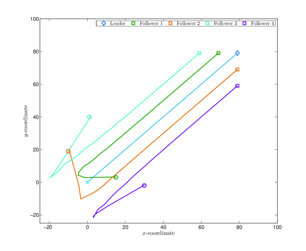
The objective is to design a distributed control law such that the leader and the four followers will asymptotically form a geometric pattern as shown in Figure 1, or mathematically,

		$\displaystyle\lim_{t\to\infty}\left(\left[\begin{array}[]{c}x_{i}(t)\\ y_{i}(t)\\ \end{array}\right]-\left[\begin{array}[]{c}x_{0}(t)\\ y_{0}(t)\\ \end{array}\right]\right)=\left[\begin{array}[]{c}x_{di}\\ y_{di}\\ \end{array}\right]$		(35)
		$\displaystyle\lim_{t\to\infty}\left(\left[\begin{array}[]{c}w_{xi}(t)\\ w_{yi}(t)\\ \end{array}\right]-\left[\begin{array}[]{c}w_{x0}\\ w_{y0}\\ \end{array}\right]\right)=0,\quad i=1,2,3,4$		(40)

in which $[x_{di},y_{di}]^{T},i=1,2,3,4$ , denotes the desired constant relative position between the $i$ th follower and the leader.

Refer to caption — Figure 1: The desired leader-following formation of mobile robots

Define the regulated output of each follower as

e_{i}(t)=\left[\begin{array}[]{c}x_{i}(t)-x_{di}\\ y_{i}(t)-y_{di}\\ \end{array}\right]-\left[\begin{array}[]{c}x_{0}(t)\\ y_{0}(t)\\ \end{array}\right],\quad i=1,2,3,4.

(41)

Then, the system composed of (V) and (41) is in the form of (IV-A) with the state $[x_{i}-x_{di},y_{i}-y_{di},w_{xi},w_{yi}]^{T}$ , regulated output $e_{i}$ , control input $u_{i}=[u_{xi},u_{yi}]^{T}$ , and various matrices given by

	$\displaystyle A_{i}$	$\displaystyle=\left[\begin{array}[]{cc}1&1\\ 0&1\\ \end{array}\right]\otimes I_{2},\quad B_{i}=\left[\begin{array}[]{c}0\\ 1\\ \end{array}\right]\otimes I_{2},\quad E_{i}=\mathbf{0}_{4\times 4}$
	$\displaystyle C_{i}$	$\displaystyle=\left[\begin{array}[]{cc}1&0\\ \end{array}\right]\otimes I_{2},\quad D_{i}=\mathbf{0}_{2\times 2},\quad F_{i}=-\left[\begin{array}[]{cc}1&0\\ \end{array}\right]\otimes I_{2}.$

In fact, the objective in (35) can be achieved if the corresponding cooperative output regulation problem is solvable.

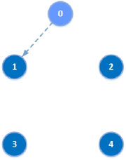
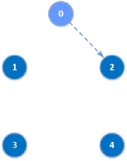
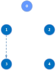
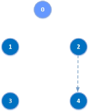
The switching digraph $\bar{\mathcal{G}}_{\sigma(t)}$ is described in Figure 2 and is dictated by the following switching signal:

\sigma(t)=\begin{cases}1,&\textrm{if}\quad t=8s+0\ \textrm{or}\ 8s+1\\ 2,&\textrm{if}\quad t=8s+2\ \textrm{or}\ 8s+3\\ 3,&\textrm{if}\quad t=8s+4\ \textrm{or}\ 8s+5\\ 4,&\textrm{if}\quad t=8s+6\ \textrm{or}\ 8s+7\end{cases}

where $s=0,1,2,\ldots$ .

It can be easily verified that Assumptions 1 to 4 are all satisfied. Therefore, by Theorems 3, this leader-following formation problem can be solved by a distributed control law of the form (24). Simulation of the closed-loop system is performed with $K_{xi}=\left[\begin{array}[]{cc}-0.7&-1.9\\ \end{array}\right]\otimes I_{2},i=1,2,3,4$ , $(x_{d1},y_{d1})=(-10,0)$ , $(x_{d2},y_{d2})=(0,-10)$ , $(x_{d3},y_{d3})=(-20,0)$ , $(x_{d4},y_{d4})=(0,-20)$ , $v(0)=[0,0,1,1]^{T}$ , $(x_{1}(0),y_{1}(0))=(15,3)$ , $(x_{2}(0),y_{2}(0))=(-10,19)$ , $(x_{3}(0),y_{3}(0))=(1,40)$ , $(x_{4}(0),y_{4}(0))=(30,-2)$ , and other randomly generated initial conditions. We let $a_{ij}(t)=1,i,j=0,1,2,3,4,$ whenever $(j,i)\in\bar{\mathcal{E}}_{\sigma(t)}$ . The trajectories of the mobile robots are shown in Figure 3.

Remark 9

In this example, the leader’s system matrix is not marginally stable. Thus, as explained in Remark 4, the approach of [20] is not applicable.

VI Conclusion

In this paper, we have developed a discrete-time distributed observer and a discrete-time adaptive distributed observer over jointly connected switching networks. By employing the discrete-time distributed observer, we have solved the cooperative output regulation problem of a discrete-time linear multi-agent system over jointly connected switching networks.

Appendix

A digraph $\mathcal{G}=\left(\mathcal{V},\mathcal{E}\right)$ consists of a finite set of nodes $\mathcal{V}=\{1,\ldots,N\}$ and an edge set $\mathcal{E}\subseteq\mathcal{V}\times\mathcal{V}$ . An edge of $\mathcal{E}$ from the node $j$ to the node $i$ is denoted by $(j,i)$ , and the node $j$ is called a neighbor of the node $i$ . Then, $\mathcal{N}_{i}=\left\{j\in\mathcal{V}\ |\ (j,i)\in\mathcal{E}\right\}$ is called the neighbor set of the node $i$ . The edge $(i,j)$ is called undirected if $(i,j)\in\mathcal{E}$ implies $(j,i)\in\mathcal{E}$ . The digraph $\mathcal{G}$ is called undirected if every edge in $\mathcal{E}$ is undirected. If the digraph contains a set of edges of the form $\{(i_{1},i_{2})$ , $(i_{2},i_{3})$ , $\ldots$ , $(i_{k-1},i_{k})\}$ , then this set is called a directed path of $\mathcal{G}$ from the node $i_{1}$ to the node $i_{k}$ , and the node $i_{k}$ is said to be reachable from the node $i_{1}$ . A digraph $\mathcal{G}_{s}=(\mathcal{V}_{s},\mathcal{E}_{s})$ is a subgraph of $\mathcal{G}=\left(\mathcal{V},\mathcal{E}\right)$ if $\mathcal{V}_{s}\subseteq\mathcal{V}$ and $\mathcal{E}_{s}\subset\mathcal{E}\cap(\mathcal{V}_{s}\times\mathcal{V}_{s})$ .

The weighted adjacency matrix of a digraph $\mathcal{G}$ is a nonnegative matrix $\mathcal{A}=[a_{ij}]_{i,j=1}^{N}\in\mathbb{R}^{N\times N}$ , where $a_{ii}=0$ and $a_{ij}>0,i\neq j$ , if and only if $(j,i)\in\mathcal{E}$ . Given a set of $n_{0}$ digraphs $\left\{\mathcal{G}_{i}=(\mathcal{V},\mathcal{E}_{i}),i=1,\ldots,n_{0}\right\}$ , the digraph $\mathcal{G}=\left(\mathcal{V},\mathcal{E}\right)$ with $\mathcal{E}=\bigcup_{i=1}^{n_{0}}\mathcal{E}_{i}$ is called the union of the digraphs $\mathcal{G}_{i}$ , denoted by $\mathcal{G}=\bigcup_{i=1}^{n_{0}}\mathcal{G}_{i}$ .

We call a time function $\sigma:\mathbb{Z}^{+}\mapsto\mathcal{P}=\{1,2,\ldots,n_{0}\}$ a piecewise constant switching signal if there exists a sequence $\{t_{j},j=0,1,2,\ldots\}$ satisfying $t_{0}=0,t_{j+1}-t_{j}\geq d$ for some positive integer $d$ such that, for all $t\in[t_{j},t_{j+1})$ , $\sigma(t)=p$ for some $p\in\mathcal{P}$ . $n_{0}$ is some positive integer, $\mathcal{P}$ is called the switching index set, $t_{j}$ is called the switching instant, and $d$ is called the dwell time. Given $\sigma(t)$ and a set of digraphs $\mathcal{G}_{i}=(\mathcal{V},\mathcal{E}_{i})$ , $i=1,\ldots,n_{0}$ , with the corresponding weighted adjacency matrices denoted by $\mathcal{A}_{i}$ , $i=1,\ldots,n_{0}$ , we call the time-varying digraph $\mathcal{G}_{\sigma(t)}=\left(\mathcal{V},\mathcal{E}_{\sigma(t)}\right)$ a switching digraph, and denote its weighted adjacency matrix by $\mathcal{A}_{\sigma(t)}$ .

References

[1] H. Cai and J. Huang, “The leader-following consensus for multiple uncertain Euler-Lagrange systems with an adaptive distributed observer,” IEEE Transactions on Automatic Control, vol. 61, no. 10, pp. 3152–3157, 2016.
[2] E. J. Davison, “The robust control of a servomechanism problem for linear time-invariant multivariable systems,” IEEE Transactions on Automatic Control, vol. 21, no. 1, pp. 25–34, 1976.
[3] B. A. Francis, “The linear multivariable regulator problem,” SIAM Journal on Control and Optimization, vol. 15, no. 3, pp. 486–505, 1977.
[4] K. Hengster-Movrica, K. You, F. L. Lewis, and L. Xie, “Synchronization of discrete-time multi-agent systems on graphs using Riccati design,” Automatica, vol. 49, no. 2, pp. 414–423, 2013.
[5] R. A. Horn and C. R. Johnson, Matrix Analysis. New York: Cambridge University Press, 1985.
[6] J. Hu and Y. Hong, “Leader-following coordination of multi-agent systems with coupling time delays,” Physica A: Statistical Mechanics and its Applications, vol. 374, no. 2. pp. 853–863, 2007.
[7] J. Huang, Nonlinear Output Regulation: Theory and Applications. Philadelphia, PA: SIAM, 2004.
[8] J. Huang, “The cooperative output regulation problem of discrete-time linear multi-agent systems by the adaptive distributed observer,” IEEE Transactions on Automatic Control, vol. 62, no. 4, pp. 1979–1984, 2017.
[9] J. Liu and J. Huang, ”Leader-following consensus for linear discrete-time multi-agent systems subject to static networks,” Proceedings of the 36th Chinese Control Conference, pp. 8684–8689, Dalian, China, July 26-28, 2017.
[10] T. Liu and J. Huang, “A discrete-time recurrent neural network for solving rank-deficient matrix equations with an application to output regulation of linear systems,” IEEE Transactions on Neural Networks and Learning Systems, vol. 29, no. 6, pp. 2271–2277, 2018.
[11] T. Liu and J. Huang, “Adaptive cooperative output regulation of discrete-time linear multi-agent systems by a distributed feedback control law,” IEEE Transactions on Automatic Control, vol. 63, no. 12, pp. 4383–4390, 2018.
[12] L. Moreau, “Stability of multiagent systems with time-dependent communication links,” IEEE Transactions on Automatic Control, vol. 50, no. 2, pp. 169–182, 2005.
[13] W. Ni and D. Cheng, “Leader-following consensus of multi-agent systems under fixed and switching topologies,” Systems & Control Letters, vol. 59, no. 3, pp. 209–217, 2010.
[14] J. Qin, H. Gao, and C. Yu, “On discrete-time convergence for general linear multi-agent systems under dynamic topology,” IEEE Transactions on Automatic Control, vol. 59, no. 4, pp. 1054–1059, 2014.
[15] J. Qin, H. Gao, and W. X. Zheng, “Exponential synchronization of complex networks of linear systems and nonlinear oscillators: A unified analysis,” IEEE Transactions on Neural Networks Learning Systems, vol. 26, no. 3, pp. 510–521, 2015.
[16] W. J. Rugh, Linear System Theory, Second Edition. Upper Saddle River, NJ: Prentice Hall, 1996.
[17] Y. Su and J. Huang, “Cooperative output regulation of linear multi-agent systems,” IEEE Transactions on Automatic Control, vol. 57, no. 4, pp. 1062–1066, 2012.
[18] Y. Su and J. Huang, “Cooperative output regulation with application to multi-agent consensus under switching network,” IEEE Transactions on Systems, Man and Cybernetics-Part B: Cybernetics, vol. 42, no. 3, pp. 864–875, 2012.
[19] Y. Yan and J. Huang, “Cooperative output regulation of discrete-time linear time-delay multi-agent systems,” IET Control Theory & Applications, vol. 10, no. 16, pp. 2019–2026, 2016.
[20] Y. Yan and J. Huang, “Cooperative output regulation of discrete-time linear time-delay multi-agent systems under switching network,” Neurocomputing, vol. 241, pp. 108–114, 2017.

	$\displaystyle\\|\zeta(t)\\|$	$\displaystyle\leq\left\\|\left(\Phi(t,t_{0})\otimes S^{t-t_{0}}\right)\right\\|\\|\zeta(t_{0})\\|$
		$\displaystyle=\left\\|\Phi(t,t_{0})\right\\|\left\\|S^{t-t_{0}}\right\\|\ \\|\zeta(t_{0})\\|$
		$\displaystyle<\alpha_{1}\alpha(\epsilon)\left(\rho(S)+\epsilon\right)^{t-t_{0}}r_{1}^{t-t_{0}}\ \\|\zeta(t_{0})\\|$
		$\displaystyle=\alpha_{2}r_{2}^{t-t_{0}}\ \\|\zeta(t_{0})\\|,\qquad t\geq t_{0}$