Discriminant indicator with generalized rotational symmetry
Abstract
Discriminant indicators with generalized inversion symmetry are computed only from data at the high-symmetry points. They allow a systematic search for exceptional points. In this paper, we propose discriminant indicators for two- and three-dimensional systems with generalized -fold rotational symmetry (, ). As is the case for generalized inversion symmetry, the indicator taking a nontrivial value predicts the emergence of exceptional points and loops without ambiguity of the reference energy. A distinct difference from the case of generalized inversion symmetry is that the indicator with generalized -fold rotational symmetry (, ) can be computed only from data at two of four high-symmetry points in the two-dimensional Brillouin zone. Such a difference is also observed in three-dimensional systems. Furthermore, we also propose how to fabricate a two-dimensional system with generalized four-fold rotational symmetry for an electrical circuit.
I Introduction
In recent decades, many efforts have been devoted to understanding the topological properties of wavefunctions [1, 2, 3, 4, 5, 6, 7, 8]. In particular, it turns out that symmetry enriches topological structure [9], which is exemplified by topological insulators with time-reversal symmetry [10, 11, 12, 13, 14, 15] and topological crystalline materials [16, 17, 18, 19, 20, 21, 22, 23, 24]. Intriguingly, crystalline symmetry also plays a key role in determining topological properties. For instance, in the presence of the inversion symmetry and time-reversal symmetry, the topological invariant can be computed only from the parity eigenvalues at high-symmetry points in the Brillouin zone (BZ) [17]. This notion is generalized in Refs. [25, 26, 27, 28, 29] which introduced symmetry indicators as powerful tools for the systematic search for topological materials.
In parallel with this progress, recent extensive studies have opened up a new arena of topological physics: non-Hermitian systems [30, 31, 32, 33, 34, 35, 36, 37]. In these systems, the eigenvalues of the Hamiltonian may become complex, which induces exotic phenomena [38, 39, 40, 41, 42, 43, 44, 45, 46, 47, 48, 49, 50, 51] such as the emergence of exceptional points [52, 53, 54, 55, 56, 57, 58, 59, 60, 61] and skin effects [62, 63, 64, 65, 66, 67, 68, 69, 70, 71, 72]. At the exceptional points, non-Hermitian topological properties protect band touching for both of the real and imaginary parts of the eigenvalues which are further enriched by symmetry [73, 74, 75, 76, 77, 78]. The skin effects result in anomalous sensitivity of energy spectrum on the presence or absence of boundaries [62, 63, 64, 66, 65, 67, 68, 69]. The exceptional points and skin effects have been reported for a wide range of systems such as open quantum systems [79, 80, 53, 81, 82], electrical circuits [83, 84, 85, 86, 87, 88], phononic systems [89, 90, 91, 92], photonic crystals [93, 94, 95, 96], and so on.
For the systematic search for non-Hermitian topological systems, symmetry indicators are powerful tools. Indeed, recent works have introduced indicators for non-Hermitian systems [70, 82, 97, 98, 99, 100]. Among them, the discriminant indicator [101] captures exceptional points without ambiguity of the reference energy.
Despite its usefulness, the discriminant indicator is introduced only for systems with generalized inversion symmetry [101]. For the systematic search for exceptional points, the extension to other symmetries is crucial.
In this paper, we extend the indicator to systems with generalized -fold rotational () symmetry for , . The indicators successfully capture the exceptional points in two dimensions without ambiguity of the reference energy, which is demonstrated by systematic analysis of toy models. We also introduce indicators which capture exceptional loops in the three-dimensional BZ. In contrast to the case with the generalized inversion symmetry [101], the indicator with generalized -fold rotational symmetry (, ) can be computed only from data at two of the four high-symmetry points in the two-dimensional BZ. Such a difference is also observed in three-dimensional systems. We also show that the nontrivial value of the discriminant indicator with generalized symmetry in three dimensions predicts the merging of the exceptional loops at the line specified by or . Moreover, we propose an experimental realization of the topoelectrical system with generalized symmetry.
The rest of this paper is organized as follows. In Sec. II, we derive the indicators for systems with generalized symmetry (, ). In Sec. III, we demonstrate that these indicators capture exceptional points and loops by numerically analyzing toy models with generalized symmetry (, ). In Sec. IV, we experimentally realize the topoelectrical circuit with generalized symmetry. In Sec. V, we present a summary of this paper.
II Discriminant indicator with generalized rotational symmetry
In this section, we derive indicators for systems with generalized rotational symmetry. In Sec. II.1, along with a definition of generalized inversion symmetry, we provide an overview of our main results. The detailed derivation is provided in Secs. II.2-II.4. In Sec. II.5, we also discuss indicators for exceptional loops in three-dimensional systems.
II.1 Overview
Consider an -Hamiltonian for two-dimensional systems with generalized symmetry under the periodic boundary condition [70, 98, 72, 99, 97, 101, 51, 100, 61]. In this case, the Hamiltonian satisfies
| (1) |
with
| (2) |
and a unitary operator satisfying .
The above non-Hermitian Hamiltonian may host exceptional points which are characterized by the discriminant number [59, 60, 78]
| (3) |
The integral is taken along a closed path in the BZ. The discriminant of the characteristic polynomial is defined as
| (4) |
Here, denote the eigenvalues of . can be rewritten as
| (5) |
with [102, 103]. Clearly, is determined by the coefficients of the characteristic polynomial. If takes a non-zero value, vanishes at a point inside of the loop. Such a point corresponds to an exceptional point because Eq. (4) indicates the band touching on this point.
In the presence of the generalized symmetry, the discriminant satisfies
| (6) |
which is proven in Sec. II.2.
By making use of Eq. (6), we obtain discriminant indicators for two-dimensional systems with generalized symmetry (, ),
| (7a) | |||
| (7b) |
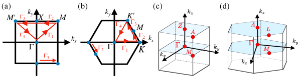
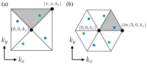
Here, and denote the discriminant number computed along the closed path illustrated in Fig. 1(a) [Fig. 1(b)]. Symbols and denote the high-symmetry points in the BZ [see Fig. 1]. Because of the constraint written in Eq. (6), the discriminant becomes real at and points.
We note that for , the problem is reduced to the case for the generalized inversion symmetry, which is discussed in Appendix A. For systems with generalized symmetry, the Hamiltonian becomes Hermitian 111 This can be seen as follows, .. In Secs. II.3 and II.4, we derive these indicators. These indicators can be computed without the input of the reference energy, and predict the presence of exceptional points.
II.2 Constraints on the discriminant with generalized rotational symmetry
For the systems with generalized symmetry, the polynomial satisfies
| (8) |
Here, we have used and . We note that the discriminant can be computed only from coefficients of the polynomial. It results in Eq. (6). It is straight forward to extend the above arguments to three-dimensional cases. Specifically, for three-dimensional systems with generalized symmetry about the axis, the discriminant satisfies
| (9) |
with .
II.3 Two-dimensional system with generalized fourfold rotational symmetry
In order to derive Eq. (7a), let us consider the discriminant number evaluated along the closed path illustrated in Fig. 1(a). This integral can be decomposed into integrals along the path (),
| (10) |
Here, () are the paths between the high-symmetry points [see Fig. 1(a)]. First, we note that vanishes because applying the generalized operator twice maps the path to the path which is equivalent to the path [see Fig. 1(a)] due to the periodicity of the BZ.
Second, let us evaluate . The integration of along the path is mapped to that of along the opposite direction of by the generalized symmetry. As a result, the integration is simplified as
| (11) |
with some integer . From the second to the third lines, we have used Eq. (6). We note that this discussion can be extended to the cases of generalized symmetry.
From these results, we obtain the relation
| (12) |
Here, we used the fact that is real at and points because of Eq. (6). Therefore, we obtain the discriminant indicator with generalized symmetry in Eq. (7a). We note that even if the exceptional points exist on the red line in Fig. 1(a), we can avoid by the continuous deformation of the integration path [24]. We also note that if , exceptional points emerge at these points.
II.4 Two-dimensional system with generalized sixfold rotational symmetry
In order to derive Eq. (7b), let us consider the discriminant number composed along the closed path illustrated in Fig. 1(b). We decompose the path for the integral into four paths () in a similar way to the previous section [see Eq. (10)].
Firstly, we discuss the integration of in a similar way to the previous case [see Eq. (11)]. In the presence of the generalized symmetry, the integration of along is mapped to the one of along . Additionally, from the periodicity in the BZ, this integration is mapped to one along the opposite direction of . Thus, in a similar way to the previous case, is simplified as
| (13) |
with some integer .
Secondly, let us simplify . The integration of along is mapped to the integration of along the opposite direction of by the generalized operator. Hence, the integration is
| (14) |
with some integer .
II.5 Three-dimensional system
Let us see the discriminant number in the three-dimensional BZ and exceptional points from loops. In the presence of generalized symmetry about the axis, the following indicator captures the exceptional loops crossing one of the planes at and ;
| (15) |
Here, , , , and denote high-symmetry points as shown in Fig. 1(c). We note that , , , and are real because of Eq. (9). All possible configurations of giving are shown in Appendix B. The above indicator is obtained by applying the argument in Sec. II.3 to the two-dimensional subsystems at and where generalized symmetry is preserved. In a similar way, we can introduce the indicator for systems with generalized symmetry,
| (16) |
where , , , and are high-symmetry points in Fig. 1(d). We note that , , , and are real because of Eq. (9).
III Applications to toy models
In this section, we demonstrate that the discriminant indicator with generalized symmetry () predicts the existence of the exceptional points and loops by numerically analyzing the two- and three-dimensional toy models with generalized symmetry.
III.1 Two-dimensional toy model with generalized fourfold rotational symmetry
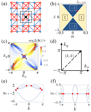
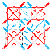
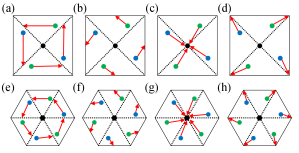
Let us consider the two-dimensional toy model with generalized symmetry in Fig. 2(a), whose Hamiltonian is defined in Appendix C. In Fig. 2(a), the red (blue) dots denote the on-site potentials (). The red (blue) lines denote the hoppings ().
The above model respects generalized symmetry whose rotation axis is illustrated by a cross in Fig. 2(a). The explicit form of is written in Appendix C.
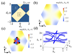
The numerical results for discriminant indicators are displayed in Fig. 2(b). The discriminant indicator takes vales of and in yellow and blue regions, respectively. We note that vanishes for or since vanishes at the high-symmetry point in the BZ. Additionally, at the boundary of the phases, vanishes for the same reason. For , the exceptional points can be observed by computing . As an example, we show the map of in momentum space for [see Fig. 2(c)]. Green and black dots in Fig. 2(c) represent exceptional points characterized by and , respectively. This result indicates that the discriminant number along the path in Fig. 1(a) takes a value of .
III.2 Two-dimensional toy model with generalized sixfold rotational symmetry
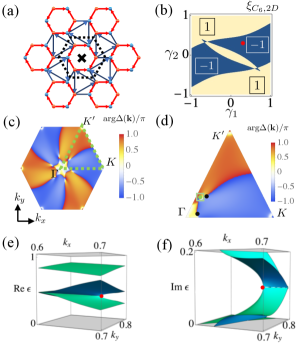
We consider the two-dimensional toy model with generalized symmetry in Fig. 3(a), whose Hamiltonian is defined in Appendix C. In this figure, the red (blue) dots denote the on-site potentials (). The red (blue) lines denote the non-reciprocal hoppings. Specifically, the hopping along the red (blue) arrows is (). The hopping opposite to the red (blue) arrows is (). For the blue lines without arrows, the hopping is for both directions.
The above model respects generalized symmetry whose rotation axis is illustrated by a cross in Fig. 3(a). The explicit form of is written in Appendix C.
We show the numerical result for the discriminant indicator in Eq. (7b) for [see Fig. 3(b)]. In Fig. 3(b), there exist two phases where the discriminant indicator takes values of (yellow area) and (blue area). We note that vanishes for and since vanishes at the high-symmetry point in the BZ. Additionally, at the boundary between phases, vanishes for the same reason. In the blue-colored region, the indicator predicts the presence of exceptional points. To be concrete, we compute in the momentum space for [see Figs. 3(c) and 3(d)]. Green and black dots in Fig. 3(d) represent exceptional points characterized by and , respectively. Figure 3(d) indicates that the discriminant number computed along the path in Fig. 1(b) takes a value of .
III.3 Three-dimensional toy model with generalized fourfold rotational symmetry
Consider the three-dimensional toy model with generalized fourfold rotational symmetry whose Hamiltonian reads
| (17) |
with
| (18a) | ||||
| (18b) | ||||
| (18c) | ||||
Here, (, , ) denote the Pauli matrices. The above model respects generalized symmetry about the axis with .
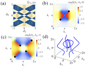
Figure 4(a) displays the numerical result for the discriminant indicator . In Fig. 4(a), there exist two phases where the discriminant indicator takes values of (yellow area) and (blue area). For , the exceptional loops crossing the plane for or can be obtained by computing the map of . As an example, we show the maps of and in momentum space for [see Figs. 4(b) and 4(c)]. In Figs. 4(b) and 4(c), green and black dots represent exceptional loops characterized by and , respectively. By comparing these figures, we obtain the emergence of the exceptional loops crossing the plane for .
Figure 4(d) displays the momentum points satisfying , indicating the emergence of exceptional loops. We note that exceptional loops predicted by the nontrivial value of merge at the line specified by or , originating from the symmetry constraint on the exceptional points for fixed in three dimensions (for more details see Appendix D).
III.4 Three-dimensional toy model with generalized sixfold rotational symmetry
Consider the three-dimensional toy model with generalized sixfold rotational symmetry whose Hamiltonian reads
| (19) |
with
| (20a) | ||||
| (20b) | ||||
| (20c) | ||||
Here, and are defined as
| (21a) | ||||
| (21b) | ||||
The above model respects generalized symmetry about the axis with .
Figure 5(a) displays the numerical result of the discriminant . In Fig. 5(a), there exist two phases where the discriminant indicator takes values of (yellow area) and (blue area). For , the exceptional loops crossing the plane for or can be obtained by computing the map of . As an example, we show the maps of and in the momentum space for [see Figs. 5(b) and 5(c)]. In Fig. 5(c), green and black dots represent exceptional loops characterized by and , respectively. By comparing Fig. 5(b) with 5(c), we obtain the emergence of the exceptional loops crossing the plane for .
Figure 5(d) displays the momentum points satisfying , indicating the emergence of exceptional loops. We note that, in contrast to the case of generalized symmetry in Sec. III.3, generalized symmetry does not predict the merging of the exceptional loops since the exceptional loops can cross the boundary of the BZ (for more details see Appendix D).
IV Topoelectrical systems with generalized fourfold rotational symmetry
We have shown that our indicators capture the exceptional points and loops in toy models. In this section, we discuss the relevance of generalized symmetry to the topoelectrical circuits [105, 106, 87].
Consider the two-dimensional topoelectrical circuit with generalized symmetry in Fig. 6. To describe this system, under the periodic boundary condition, we define the voltages at each node as and electric currents between the node and the power source as . Here, denotes the frequency of the currents from the power source into the node. The admittance of the red (blue) resistors shown in Fig. 6 is () with and . The admittance of red (blue) inductors is (), with and . The relation between and is
| (22) |
Here, denotes the admittance matrix,
| (23) |
We note that the constant diagonal terms just shift the band structure and do not contribute to the emergence of exceptional points. Thus, we define by removing the constant diagonal terms of the admittance matrix,
| (24) |
Clearly, corresponds to the Hamiltonian in Sec. III.1.
V Summary
Extending the argument of the work in [101], we have introduced the discriminant indicators for two- and three-dimensional systems with generalized symmetry (, ). In two dimensions, the indicators can be computed from the parity of the discriminant at the and points [see Eqs. (7a) and (7b)], which is in contrast to the case of generalized inversion symmetry. These indicators taking a nontrivial value predict the emergence of exceptional points and exceptional loops without the input of the reference energy. We have numerically confirmed that these indicators capture the exceptional points and the loops for two- and three-dimensional toy models.
Acknowledgements.
The authors thank R. Okugawa for fruitful discussion. This work is supported by JSPS KAKENHI Grants No. JP17H06138, No. JP20H04627, and No. JP21K13850 and also by JST CREST, Grant No. JPMJCR19T1, Japan.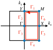
Appendix A Discriminant indicator with generalized twofold rotational symmetry
We briefly discuss the indicators for systems with generalized symmetry, although the problem is reduced to the one for generalized inversion symmetry.
With generalized symmetry in two-dimensional systems, the discriminant number is simplified to the computation at the high-symmetry points in the BZ [101]. This symmetry enables us to rewrite Eq. (3) as the discriminant indicator,
| (25) |
where denotes the discriminant number defined along the path in Fig. 7. Symbols , , , and denote the high-symmetry points [see Fig. 7]. We note that , , , and are real because of Eq. (6).
We see the derivation of Eq. (25). Let us consider the discriminant number [see Eq. (4)] composed along the closed path illustrated in Fig. 7. In a way similar to what we did in Sec. II.3, we decompose the closed path into six parts. The integral for the paths () is denoted by () in Eq. (10).
We note that holds due to the periodicity of the BZ. We also note that is simplified as
| (26) |
with some integer . This is because is mapped to by applying the operator of generalized symmetry. In a similar way, we have
| (27) |
with some integer .
Putting Eqs. (26) and (27) together, we obtain Eq. (25). Here, we have used the fact that is real at the , , , and points because of Eq. (6).
Appendix B Specific configuration with the nontrivial value of the discriminant indicator
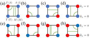
In this appendix, we illustrate the specific configuration yielding (see Fig. 8). With this nontrivial value of the indicators, the exceptional loops emerge crossing one of the planes for or exist. For example, in Fig. 8(a), there exist an exceptional loop crossing the plane for , and two loops crossing both of the planes for and . In this case, at the plane for , the indicator for two-dimensional systems takes a trivial (nontrivial) value. This result indicates that the discriminant indicator takes a value of .
Appendix C Details of the Hamiltonian in toy models
Here, we show the details of the Hamiltonian in Sec. III. The bulk Hamiltonian describing the toy model in Fig. 2(a) is
| (28) |
This model preserves generalized symmetry [see Eq. (1)] where is defined as
| (29) |
Additionally, the bulk Hamiltonian describing the toy model in Fig. 3(a) is
| (30) |
Here, and are the unit vectors.
This model preserves generalized symmetry [see Eq. (1)] where is defined as
| (31) |
Appendix D The merging of exceptional loops
In this appendix, we show the details of the merging of exceptional loops arising by generalized rotational symmetry in three dimensions. Consider the case in which the discriminant indicator (, ) takes the nontrivial value. In this case, the exceptional loops emerge, meaning that the presence of the exceptional point in a two-dimensional subspace is specified by a given (see Fig. 9). We note that an odd number of exceptional points exist in the shaded area in the BZ due to the nontrivial value of the two-dimensional indicator for this subspace. We also note that applying the generalized rotation, an exceptional point is mapped to another one with the opposite sign of the velocity (see Fig. 9).
The merging of the exceptional loops observed in Fig. 4(d) can be understood by shifting . Because of the indicator taking a value of , the exceptional points observed in Fig. 9(a) should annihilate each other. Such annihilation is allowed only at and in the presence of generalized symmetry. In the following, we see the details.
Consider a proper where the exceptional points emerge [see Fig. 9(a)]. Shifting , we can see that these exceptional points in the shaded area move to the boundaries, which is categorized into four cases [see Figs. 10(a)10(d)]. In the case illustrated in Fig. 10(a), the exceptional point does not meet another one, and thus, pair annihilation does not occur. In the case illustrated in Fig. 10(b), the exceptional point meets another one but with the same vorticity, and thus, pair annihilation does not occur. In the case illustrated in Figs. 10(c) and 10(d), the exceptional point meets another one with opposite vorticities. The above argument elucidates that two exceptional loops merge at the line specified by and .
In a similar way, let us consider the case of generalized symmetry. In this case, the indicator does not necessary mean the merging of exceptional loops. Let us illustrate the details. As is the case for the generalized symmetry, the movement of the exceptional point for the pair annihilation is categorized into four cases in Figs. 10(e)-10(h). In the case illustrated in Fig. 10(e), the exceptional point does not meet another one, and thus, pair annihilation does not occur. In the case illustrated in Figs. 10(f) and 10(g), the exceptional point meets another one with the opposite vorticity. Thus, pair annihilation occurs. In the case illustrated in Fig. 10(h), the exceptional point meets another one with the same vorticity, and thus, pair annihilation does not occur. The above argument indicates that the indicator does not necessarily mean the merging of the exceptional points.
References
- Hatsugai [1993a] Y. Hatsugai, Phys. Rev. Lett. 71, 3697 (1993a).
- Hatsugai [1993b] Y. Hatsugai, Phys. Rev. B 48, 11851 (1993b).
- Kane and Mele [2005] C. L. Kane and E. J. Mele, Phys. Rev. Lett. 95, 146802 (2005).
- Teo et al. [2008] J. C. Y. Teo, L. Fu, and C. L. Kane, Phys. Rev. B 78, 045426 (2008).
- Qi et al. [2008] X.-L. Qi, T. L. Hughes, and S.-C. Zhang, Phys. Rev. B 78, 195424 (2008).
- Hasan and Kane [2010] M. Z. Hasan and C. L. Kane, Rev. Mod. Phys. 82, 3045 (2010).
- Qi and Zhang [2011] X.-L. Qi and S.-C. Zhang, Rev. Mod. Phys. 83, 1057 (2011).
- Sato and Fujimoto [2016] M. Sato and S. Fujimoto, Journal of the Physical Society of Japan 85, 072001 (2016).
- Chiu et al. [2016] C.-K. Chiu, J. C. Y. Teo, A. P. Schnyder, and S. Ryu, Rev. Mod. Phys. 88, 035005 (2016).
- Fu and Kane [2006] L. Fu and C. L. Kane, Phys. Rev. B 74, 195312 (2006).
- Fu et al. [2007] L. Fu, C. L. Kane, and E. J. Mele, Phys. Rev. Lett. 98, 106803 (2007).
- Moore and Balents [2007] J. E. Moore and L. Balents, Phys. Rev. B 75, 121306 (2007).
- Zhang et al. [2009] H. Zhang, C.-X. Liu, X.-L. Qi, X. Dai, Z. Fang, and S.-C. Zhang, Nature physics 5, 438 (2009).
- Roy [2009] R. Roy, Phys. Rev. B 79, 195322 (2009).
- Hsieh et al. [2009] D. Hsieh, Y. Xia, D. Qian, L. Wray, F. Meier, J. H. Dil, J. Osterwalder, L. Patthey, A. V. Fedorov, H. Lin, A. Bansil, D. Grauer, Y. S. Hor, R. J. Cava, and M. Z. Hasan, Phys. Rev. Lett. 103, 146401 (2009).
- Zak [1989] J. Zak, Phys. Rev. Lett. 62, 2747 (1989).
- Fu and Kane [2007] L. Fu and C. L. Kane, Phys. Rev. B 76, 045302 (2007).
- Hughes et al. [2011] T. L. Hughes, E. Prodan, and B. A. Bernevig, Phys. Rev. B 83, 245132 (2011).
- Fu [2011] L. Fu, Phys. Rev. Lett. 106, 106802 (2011).
- Fang et al. [2012] C. Fang, M. J. Gilbert, and B. A. Bernevig, Phys. Rev. B 86, 115112 (2012).
- Slager et al. [2013] R.-J. Slager, A. Mesaros, V. Juričić, and J. Zaanen, Nat. Phys. 9, 98 (2013).
- Morimoto and Furusaki [2013] T. Morimoto and A. Furusaki, Phys. Rev. B 88, 125129 (2013).
- Koshino et al. [2014] M. Koshino, T. Morimoto, and M. Sato, Phys. Rev. B 90, 115207 (2014).
- Kim et al. [2015] Y. Kim, B. J. Wieder, C. L. Kane, and A. M. Rappe, Phys. Rev. Lett. 115, 036806 (2015).
- Po et al. [2017] H. C. Po, A. Vishwanath, and H. Watanabe, Nat. Commun. 8, 1 (2017).
- Kruthoff et al. [2017] J. Kruthoff, J. de Boer, J. van Wezel, C. L. Kane, and R.-J. Slager, Phys. Rev. X 7, 041069 (2017).
- Watanabe and Lu [2018] H. Watanabe and L. Lu, Phys. Rev. Lett. 121, 263903 (2018).
- Ono and Watanabe [2018] S. Ono and H. Watanabe, Phys. Rev. B 98, 115150 (2018).
- Po [2020] H. C. Po, J. Phys.: Condens. Matter 32, 263001 (2020).
- Hatano and Nelson [1996] N. Hatano and D. R. Nelson, Phys. Rev. Lett. 77, 570 (1996).
- Bender and Boettcher [1998] C. M. Bender and S. Boettcher, Phys. Rev. Lett. 80, 5243 (1998).
- Rotter [2009] I. Rotter, J. Phys. A 42, 153001 (2009).
- Sato et al. [2012] M. Sato, K. Hasebe, K. Esaki, and M. Kohmoto, Progress of Theoretical Physics 127, 937 (2012).
- Ashida et al. [2016] Y. Ashida, S. Furukawa, and M. Ueda, Phys. Rev. A 94, 053615 (2016).
- Ashida et al. [2017] Y. Ashida, S. Furukawa, and M. Ueda, Nat. Commun. 8, 15791 (2017).
- Bergholtz et al. [2021] E. J. Bergholtz, J. C. Budich, and F. K. Kunst, Rev. Mod. Phys. 93, 015005 (2021).
- Ashida et al. [2020] Y. Ashida, Z. Gong, and M. Ueda, Advances in Physics 69, 249 (2020).
- Esaki et al. [2011] K. Esaki, M. Sato, K. Hasebe, and M. Kohmoto, Phys. Rev. B 84, 205128 (2011).
- Hu and Hughes [2011] Y. C. Hu and T. L. Hughes, Phys. Rev. B 84, 153101 (2011).
- Liang and Huang [2013] S.-D. Liang and G.-Y. Huang, Phys. Rev. A 87, 012118 (2013).
- Gong et al. [2017] Z. Gong, S. Higashikawa, and M. Ueda, Phys. Rev. Lett. 118, 200401 (2017).
- Shen et al. [2018] H. Shen, B. Zhen, and L. Fu, Phys. Rev. Lett. 120, 146402 (2018).
- Carlström and Bergholtz [2018] J. Carlström and E. J. Bergholtz, Phys. Rev. A 98, 042114 (2018).
- Liu et al. [2019] C.-H. Liu, H. Jiang, and S. Chen, Phys. Rev. B 99, 125103 (2019).
- Carlström et al. [2019] J. Carlström, M. Stålhammar, J. C. Budich, and E. J. Bergholtz, Phys. Rev. B 99, 161115 (2019).
- Okuma and Sato [2019] N. Okuma and M. Sato, Phys. Rev. Lett. 123, 097701 (2019).
- Yoshida et al. [2019a] T. Yoshida, K. Kudo, and Y. Hatsugai, Sci. Rep. 9, 16895 (2019a).
- Gong et al. [2018] Z. Gong, Y. Ashida, K. Kawabata, K. Takasan, S. Higashikawa, and M. Ueda, Phys. Rev. X 8, 031079 (2018).
- Kawabata et al. [2019a] K. Kawabata, K. Shiozaki, M. Ueda, and M. Sato, Phys. Rev. X 9, 041015 (2019a).
- Zhou and Lee [2019] H. Zhou and J. Y. Lee, Phys. Rev. B 99, 235112 (2019).
- Chen and Khanikaev [2022] K. Chen and A. B. Khanikaev, Phys. Rev. B 105, L081112 (2022).
- Zhen et al. [2015] B. Zhen, C. W. Hsu, Y. Igarashi, L. Lu, I. Kaminer, A. Pick, S.-L. Chua, J. D. Joannopoulos, and M. Soljačić, Nature (London) 525, 354 (2015).
- Lee [2016] T. E. Lee, Phys. Rev. Lett. 116, 133903 (2016).
- Leykam et al. [2017] D. Leykam, K. Y. Bliokh, C. Huang, Y. D. Chong, and F. Nori, Phys. Rev. Lett. 118, 040401 (2017).
- Kozii and Fu [2017] V. Kozii and L. Fu, arXiv:1708.05841 (2017).
- Martinez Alvarez et al. [2018] V. M. Martinez Alvarez, J. E. Barrios Vargas, and L. E. F. Foa Torres, Phys. Rev. B 97, 121401 (2018).
- Yoshida et al. [2018] T. Yoshida, R. Peters, and N. Kawakami, Phys. Rev. B 98, 035141 (2018).
- Kawabata et al. [2019b] K. Kawabata, T. Bessho, and M. Sato, Phys. Rev. Lett. 123, 066405 (2019b).
- Wojcik et al. [2020] C. C. Wojcik, X.-Q. Sun, T. c. v. Bzdušek, and S. Fan, Phys. Rev. B 101, 205417 (2020).
- Yang et al. [2021] Z. Yang, A. P. Schnyder, J. Hu, and C.-K. Chiu, Phys. Rev. Lett. 126, 086401 (2021).
- Rui et al. [2022] W. B. Rui, Z. Zheng, C. Wang, and Z. D. Wang, Phys. Rev. Lett. 128, 226401 (2022).
- Kunst et al. [2018] F. K. Kunst, E. Edvardsson, J. C. Budich, and E. J. Bergholtz, Phys. Rev. Lett. 121, 026808 (2018).
- Yao and Wang [2018] S. Yao and Z. Wang, Phys. Rev. Lett. 121, 086803 (2018).
- Yao et al. [2018] S. Yao, F. Song, and Z. Wang, Phys. Rev. Lett. 121, 136802 (2018).
- Edvardsson et al. [2019] E. Edvardsson, F. K. Kunst, and E. J. Bergholtz, Phys. Rev. B 99, 081302 (2019).
- Lee and Thomale [2019] C. H. Lee and R. Thomale, Phys. Rev. B 99, 201103 (2019).
- Borgnia et al. [2020] D. S. Borgnia, A. J. Kruchkov, and R.-J. Slager, Phys. Rev. Lett. 124, 056802 (2020).
- Zhang et al. [2020] K. Zhang, Z. Yang, and C. Fang, Phys. Rev. Lett. 125, 126402 (2020).
- Okuma et al. [2020] N. Okuma, K. Kawabata, K. Shiozaki, and M. Sato, Phys. Rev. Lett. 124, 086801 (2020).
- Okugawa et al. [2020] R. Okugawa, R. Takahashi, and K. Yokomizo, Phys. Rev. B 102, 241202 (2020).
- Okuma and Sato [2021] N. Okuma and M. Sato, Phys. Rev. Lett. 126, 176601 (2021).
- Sun et al. [2021] X.-Q. Sun, P. Zhu, and T. L. Hughes, Phys. Rev. Lett. 127, 066401 (2021).
- Budich et al. [2019] J. C. Budich, J. Carlström, F. K. Kunst, and E. J. Bergholtz, Phys. Rev. B 99, 041406 (2019).
- Okugawa and Yokoyama [2019] R. Okugawa and T. Yokoyama, Phys. Rev. B 99, 041202 (2019).
- Yoshida et al. [2019b] T. Yoshida, R. Peters, N. Kawakami, and Y. Hatsugai, Phys. Rev. B 99, 121101 (2019b).
- Zhou et al. [2019] H. Zhou, J. Y. Lee, S. Liu, and B. Zhen, Optica 6, 190 (2019).
- Mandal and Bergholtz [2021] I. Mandal and E. J. Bergholtz, Phys. Rev. Lett. 127, 186601 (2021).
- Delplace et al. [2021] P. Delplace, T. Yoshida, and Y. Hatsugai, Phys. Rev. Lett. 127, 186602 (2021).
- Jin and Song [2009] L. Jin and Z. Song, Phys. Rev. A 80, 052107 (2009).
- San-Jose et al. [2016] P. San-Jose, J. Cayao, E. Prada, and R. Aguado, Scientific Reports 6, 21427 (2016).
- Xu et al. [2017] Y. Xu, S.-T. Wang, and L.-M. Duan, Phys. Rev. Lett. 118, 045701 (2017).
- Yoshida et al. [2020a] T. Yoshida, K. Kudo, H. Katsura, and Y. Hatsugai, Phys. Rev. Research 2, 033428 (2020a).
- Ezawa [2019a] M. Ezawa, Phys. Rev. B 99, 201411 (2019a).
- Hofmann et al. [2019] T. Hofmann, T. Helbig, C. H. Lee, M. Greiter, and R. Thomale, Phys. Rev. Lett. 122, 247702 (2019).
- Ezawa [2019b] M. Ezawa, Phys. Rev. B 100, 081401 (2019b).
- Yoshida et al. [2020b] T. Yoshida, T. Mizoguchi, and Y. Hatsugai, Phys. Rev. Research 2, 022062(R) (2020b).
- Hofmann et al. [2020] T. Hofmann, T. Helbig, F. Schindler, N. Salgo, M. Brzezińska, M. Greiter, T. Kiessling, D. Wolf, A. Vollhardt, A. Kabaši, C. H. Lee, A. Bilušić, R. Thomale, and T. Neupert, Phys. Rev. Research 2, 023265 (2020).
- Helbig et al. [2020] T. Helbig, T. Hofmann, S. Imhof, M. Abdelghany, T. Kiessling, L. W. Molenkamp, C. H. Lee, A. Szameit, M. Greiter, and R. Thomale, Nat. Phys. 16, 747 (2020).
- Miri and Alù [2019] M.-A. Miri and A. Alù, Science 363, eaar7709 (2019).
- Yoshida and Hatsugai [2019] T. Yoshida and Y. Hatsugai, Phys. Rev. B 100, 054109 (2019).
- Ghatak et al. [2020] A. Ghatak, M. Brandenbourger, J. van Wezel, and C. Coulais, Proceedings of the National Academy of Sciences 117, 29561 (2020).
- Scheibner et al. [2020] C. Scheibner, W. T. M. Irvine, and V. Vitelli, Phys. Rev. Lett. 125, 118001 (2020).
- Guo et al. [2009] A. Guo, G. J. Salamo, D. Duchesne, R. Morandotti, M. Volatier-Ravat, V. Aimez, G. A. Siviloglou, and D. N. Christodoulides, Phys. Rev. Lett. 103, 093902 (2009).
- Rüter et al. [2010] C. E. Rüter, K. G. Makris, R. El-Ganainy, D. N. Christodoulides, M. Segev, and D. Kip, Nat. Phys. 6, 192 (2010).
- Feng et al. [2017] L. Feng, R. El-Ganainy, and L. Ge, Nat. Photonics 11, 752 (2017).
- Isobe et al. [2021] T. Isobe, T. Yoshida, and Y. Hatsugai, Phys. Rev. B 104, L121105 (2021).
- Okugawa et al. [2021] R. Okugawa, R. Takahashi, and K. Yokomizo, Phys. Rev. B 103, 205205 (2021).
- Vecsei et al. [2021] P. M. Vecsei, M. M. Denner, T. Neupert, and F. Schindler, Phys. Rev. B 103, L201114 (2021).
- Shiozaki and Ono [2021] K. Shiozaki and S. Ono, Phys. Rev. B 104, 035424 (2021).
- Tsubota et al. [2022] S. Tsubota, H. Yang, Y. Akagi, and H. Katsura, Phys. Rev. B 105, L201113 (2022).
- Yoshida et al. [2022] T. Yoshida, R. Okugawa, and Y. Hatsugai, Phys. Rev. B 105, 085109 (2022).
- Mignotte [1992] M. Mignotte, Mathematics for computer algebra (Springer-Verlag, New York, Inc. 1992).
- Lang [2002] S. Lang, Graduate Texts in Mathematics: Algebra, Vol. 211 (Springer Science & Business Media, New York, 2002).
- Note [1] This can be seen as follows, .
- Albert et al. [2015] V. V. Albert, L. I. Glazman, and L. Jiang, Phys. Rev. Lett. 114, 173902 (2015).
- Lee et al. [2018] C. H. Lee, S. Imhof, C. Berger, F. Bayer, J. Brehm, L. W. Molenkamp, T. Kiessling, and R. Thomale, Commun. Phys. 1, 39 (2018).