Discussion of “Estimating the historical and future probabilities of large terrorist events” by Aaron Clauset and Ryan Woodard

10.1214/12-AOAS614

Discussion of “Estimating the historical and future probabilities of large terrorist events” by Aaron Clauset and Ryan Woodard

I congratulate Clauset and Woodard (2013) on a very interesting article. The authors analyze a global terrorism data set with the aim of quantifying the probability of historical and future catastrophic terrorism events. Using power law, stretched exponential and log-normal tail probability models for the severity of events (# deaths), the authors make a convincing argument that a 9/11-sized event is not an outlier among the catalog of terrorist events between 1968 and 2007. This study builds upon earlier work by Clauset, Young and Gleditsch (2007) that I also recommend for those interested in the statistical modeling of terrorism.

While there is consensus among the models employed by Clauset and Woodard that 9/11 is not an outlier ($p>0.01$), the estimates are accompanied by large confidence intervals on how likely a 9/11-sized event is. In Table 2, where the authors forecast the probability of a 9/11-sized event in 2012–2021, forecasted probabilities range from 0.04 to 0.94 depending on the model and the frequency of events over the time window. Here the uncertainty has less to  do with the model specification and more to do with uncertainty in the frequency of events over the next decade. Terrorist events do not follow a stationary Poisson process and the intensity can fluctuate greatly over a several year period of time.

The authors remark in their discussion that relaxing the stationarity assumptions and incorporating spatial and exogenous variables may help tighten the range of forecasted probabilities. I would add here that some progress has been made, in particular, on modeling terrorist event time series as nonstationary point processes [see Porter and White (2012), Lewis et al. (2012), Zammit-Mangion et al. (2012), Mohler (2013), Raghavan, Galstyan and Tartakovsky (2012)]. Terrorism event processes are history dependent and intensities exhibit correlations at timescales of weeks and months due to self-excitation [see Porter and White (2012), Lewis et al. (2012)] and exogenous effects [see Raghavan, Galstyan and Tartakovsky (2012), Mohler (2013)].

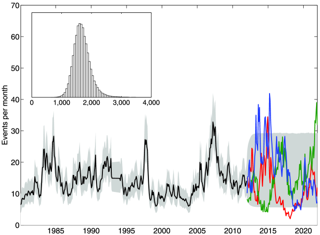
Log-Gaussian Cox processes (LGCPs) can be used to forecast the frequency of terrorist events over the next decade, allowing for mean reversion and some level of smoothness of the intensity. Here we fit the intensity of a LGCP to the time series of global terrorist attacks with 10 or more deaths from 1980 to 2011¹¹1Data source: Global Terrorism Database. using Langevin Monte Carlo [see Mohler (2013)]. The intensity of the process $\lambda_{t}=e^{x_{t}}$ is determined by a Gaussian process $x_{t}$ satisfying the mean-reverting stochastic differential equation,

We jointly sample the posterior of the intensity and model parameters and display the posterior mean and 90% range in Figure 1. For each sampled intensity, we use the terminal estimated value at the end of 2011 and the corresponding posterior parameters to simulate the intensity forward in time over the range 2012–2021. The inset in Figure 1 displays the posterior distribution of the 10 year frequency of events over 2012–2021, with most probability mass contained between 1000 and 3000 events of severity 10 or greater. This result would indicate that Clauset and Woodard’s “status quo” forecast is more likely than either the “optimistic” or “pessimistic” scenarios (it should be pointed out that our forecast of the frequency of events utilizes GTD data, whereas Clauset and Woodard use RAND-MIPT).

The probability of catastrophic terrorist events also depends on the type of weapon used. Clauset and Woodard (2013) find that the estimated historical probability of a 9/11-sized event is greatest for explosives ($p=0.37$), fire ($p=0.14$) and firearms ($p=0.12$). Given that 9/11 is categorized as “other” and involved a high degree of planning and coordination, it may not be the case that all types of terrorism can be modeled alongside “other” events as i.i.d. random variables. In this case it becomes more likely that 9/11 is an outlier, given that the confidence interval the authors provide for the historical probability of a catastrophic event of type other is $[0,0.24]$ and the mean is $p=0.06$.

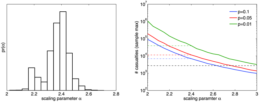
Ideally, model development should be done in collaboration with domain experts who can provide insight into whether weapon-dependent severity probabilities are realistic. Here it may be useful to consider the distribution of the sample max of competing models to determine plausibility. In Figure 2 (right) we plot the severity of the sample max as a function of the scaling parameter for the 90th, 95th and 99th percentiles. For the MLE parameter $\alpha=2.4$, the 95th percentile of the sample max is approximately 12,000 and the 99th percentile is approximately 37,000, an order of magnitude larger than 9/11 (dashed line in Figure 2). The authors note uncertainty in the estimate for $\alpha$, in particular, 15% of bootstrapped estimates cluster around $\alpha=2.2$ (see Figure 2 left). A decrease in the scaling parameter corresponds to an increase in the severity threshold separating rare from plausible. The 95th and 99th percentiles for $\alpha=2.2$ correspond to severities of 37,000 and 130,000, respectively. One question that needs to be addressed is whether events of various types, such as knife or firearm, can produce an event with $10^{4}$ or $10^{5}$ casualties. If not, then the power law or the i.i.d. assumption may not be appropriate.

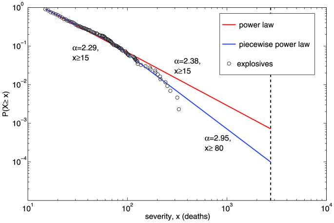
We end this discussion by analyzing events of type “explosive” that Clauset and Woodard estimate as having the highest probability ($p=0.37$) among all weapon types of producing a 9/11-sized event. In Figure 3 we plot the best fit power law model (red) using the KS estimation procedure Clauset and Woodard outline against the empirical distribution of events of type explosive. The cutoff point of the tail $x_{\mathrm{min}}$ is determined by minimizing the $L_{\infty}$ distance between the tail model CDF, $F(x;x_{\mathrm{min}})$, and the empirical CDF, $G(x;x_{\mathrm{min}})$. The tail model CDF $F$ is estimated for fixed $x_{\mathrm{min}}$ via MLE and both $F$ and $G$ are normalized to be cumulative distributions on $[x_{\mathrm{min}},\infty)$.

It should be noted that the power law model exhibits a significant deviation from the data at the “extreme” tail, that is, the $40$–$50$ events with the largest severity. A weakness of the author’s KS estimation procedure is that, for small $x_{\mathrm{min}}$, error in the extreme tail is ignored because the KS error satisfies the inequality,

and the probabilities on the right in (2) are small for large $x$, small $x_{\mathrm{min}}$ (but may be large for large $x$, large $x_{\mathrm{min}}$). Thus, the KS procedure may select a value for $x_{\mathrm{min}}$ that fits the mid-tail over a value that fits the extreme tail. This is not ideal since the goal here is to estimate the probability of the most extreme events, not mid-sized events. To give a concrete example, we fit a piecewise power law to the explosive events and plot the CDF in blue in Figure 3. The value $x=80$ is chosen by inspection for the starting point of the extreme tail, leaving $43$ events to the right. A likelihood ratio test rejects the power law in favor of the piecewise power law at the $p=0.07$ level and, furthermore, the piecewise power law has a lower KS error ($0.027$ compared to $0.033$). The odd property of the KS estimation procedure is that if the first component of the piecewise power law is removed, then the model has a worse KS error than the single power law model even though the extreme tail component is unchanged. The piecewise power law model corresponds to a historical 9/11 probability of $\approx\!0.04$, an order of magnitude smaller.

We have ignored the role of variance in our discussion of the power law fit and it is possible that $40$–$50$ events is too small of a sample size for estimating the tail. A better approach might be to compute the KS error on the extreme tail only and then choose $x_{\mathrm{min}}$ via cross-validation. Further research is needed on the selection of $x_{\mathrm{min}}$, in particular, on how to achieve a good fit in the extreme tail without overfitting.

References

- Clauset and Woodard (2013) {barticle}[author] \bauthor\bsnmClauset, \bfnmAaron\binitsA. and \bauthor\bsnmWoodard, \bfnmRyan\binitsR. (\byear2013). \btitleEstimating the historical and future probabilities of large terrorist events. \bjournalAnn. Appl. Stat. \bvolume7 \bpages1838–1865. \bptokimsref \endbibitem
- Clauset, Young and Gleditsch (2007) {barticle}[author] \bauthor\bsnmClauset, \bfnmAaron\binitsA., \bauthor\bsnmYoung, \bfnmMaxwell\binitsM. and \bauthor\bsnmGleditsch, \bfnmKristian Skrede\binitsK. S. (\byear2007). \btitleOn the frequency of severe terrorist events. \bjournalJournal of Conflict Resolution \bvolume51 \bpages58–87. \bptokimsref \endbibitem
- Lewis et al. (2012) {barticle}[author] \bauthor\bsnmLewis, \bfnmErik\binitsE., \bauthor\bsnmMohler, \bfnmGeorge\binitsG., \bauthor\bsnmBrantingham, \bfnmP Jeffrey\binitsP. J. and \bauthor\bsnmBertozzi, \bfnmAndrea L\binitsA. L. (\byear2012). \btitleSelf-exciting point process models of civilian deaths in Iraq. \bjournalSecurity Journal \bvolume25 \bpages244–264. \bptokimsref \endbibitem
- Mohler (2013) {barticle}[author] \bauthor\bsnmMohler, \bfnmGeorge\binitsG. (\byear2013). \btitleModeling and estimation of multisource clustering in crime and security data. \bjournalAnn. Appl. Stat. \bvolume7 \bpages1525–1539. \bidmr=3127957 \bptokimsref \endbibitem
- Porter and White (2012) {barticle}[mr] \bauthor\bsnmPorter, \bfnmMichael D.\binitsM. D. and \bauthor\bsnmWhite, \bfnmGentry\binitsG. (\byear2012). \btitleSelf-exciting hurdle models for terrorist activity. \bjournalAnn. Appl. Stat. \bvolume6 \bpages106–124. \biddoi=10.1214/11-AOAS513, issn=1932-6157, mr=2951531 \bptokimsref \endbibitem
- Raghavan, Galstyan and Tartakovsky (2012) {bmisc}[author] \bauthor\bsnmRaghavan, \bfnmVasanthan\binitsV., \bauthor\bsnmGalstyan, \bfnmAram\binitsA. and \bauthor\bsnmTartakovsky, \bfnmAlexander G\binitsA. G. (\byear2012). \bhowpublishedHidden Markov models for the activity profile of terrorist groups. Available at \arxivurlarXiv:1207.1497. \bptokimsref \endbibitem
- Zammit-Mangion et al. (2012) {barticle}[author] \bauthor\bsnmZammit-Mangion, \bfnmAndrew\binitsA., \bauthor\bsnmDewar, \bfnmMichael\binitsM., \bauthor\bsnmKadirkamanathan, \bfnmVisakan\binitsV. and \bauthor\bsnmSanguinetti, \bfnmGuido\binitsG. (\byear2012). \btitlePoint process modelling of the Afghan War Diary. \bjournalProc. Natl. Acad. Sci. USA \bvolume109 \bpages12414–12419. \bptokimsref \endbibitem