Disentangling Doubt in Deep Causal AI
Abstract
Accurate individual treatment-effect estimation in high-stakes applications demands both reliable point predictions and interpretable uncertainty quantification. We propose a factorized Monte Carlo Dropout framework for deep twin-network models that splits total predictive variance into representation uncertainty () in the shared encoder and prediction uncertainty () in the outcome heads. Across three synthetic covariate-shift regimes, our intervals are well-calibrated (ECE<0.03) and satisfy . Additionally, we observe a crossover—head uncertainty leads on in-distribution data but representation uncertainty dominates under shift. Finally, on a real-world twins cohort with induced multivariate shifts, only spikes on out-of-distribution samples () and becomes the primary error predictor (), while remains flat. This module-level decomposition offers a practical diagnostic for detecting and interpreting uncertainty sources in deep causal-effect models.
1 Introduction
Effective causal decision-making in domains such as finance, healthcare, and public policy requires not only accurate estimates of individual treatment effects (ITE) but also uncertainty measures that distinguish between epistemic uncertainty—due to lack of data or coverage in parts of the covariate space—and aleatoric uncertainty—due to irreducible outcome noise. In practice, selection and sampling biases frequently induce covariate-shifted subpopulations (e.g. under-represented demographic groups or clinical cohorts), making it crucial to diagnose when an ITE model is extrapolating beyond its training distribution. Existing deep-learning approaches (e.g., TARNet [1], DragonNet [2]) and Bayesian trees (e.g. BART [3], Causal Forests [4]) provide interval estimates but conflate all uncertainty into a single score, obscuring whether errors stem from encoder-level coverage gaps or head-level noise.
We address this gap by introducing a principled, module-level variance decomposition in deep twin-network architectures. Applying Monte Carlo Dropout with distinct dropout masks in the shared encoder and in each treatment-specific head yields two uncertainty components:
-
•
Representation uncertainty (), capturing epistemic doubt in the encoder’s latent covariates;
-
•
Prediction uncertainty (), capturing aleatoric noise in the outcome heads.
By the law of total variance, we obtain
We first confirm well-calibrated intervals (ECE<0.03) and variance additivity on a baseline synthetic task. Next, across three controlled covariate-shift regimes we reveal a “crossover”: on in-distribution data, total uncertainty leads error prediction (), while under strong shift representation uncertainty dominates (). Finally, on a real-world twins cohort with induced multivariate sampling bias, we show that only reliably spikes on out-of-distribution samples () and becomes the primary error signal (), whereas remains flat. This factorized framework thus provides practitioners with a clear diagnostic for detecting and interpreting layer-wise uncertainty under distributional drift.
2 Related Work
2.1 Uncertainty in Deep Learning
Estimating predictive uncertainty in deep neural networks has been a major focus across vision, language, and beyond. Gal and Ghahramani [5] showed that Monte Carlo Dropout can be interpreted as approximate Bayesian inference, providing a scalable means to capture epistemic uncertainty. Deep ensembles [6] improve on this by averaging predictions from multiple independently trained models, yielding both strong accuracy and reliable uncertainty estimates. Deep Gaussian Processes [7] stack Gaussian Process priors in multiple layers to model both epistemic and aleatoric uncertainty nonparametrically, though scalability remains a challenge. More recent work has revisited the foundational definitions of aleatoric versus epistemic uncertainty, arguing for richer taxonomies and coherence in their interpretation [8, 9].
2.2 Causal Inference and Treatment Effect Estimation
Heterogeneous treatment-effect estimation has seen extensive methodological development. Meta-learners such as the T-, S-, and X-learners [10] adapt any base learner to estimate individual treatment effects. Representation-learning approaches like TARNet [1] and DragonNet [2] mitigate selection bias by first learning a shared covariate encoder and then branching into separate treatment and control outcome heads. Bayesian methods—most notably Bayesian Additive Regression Trees (BART) [3, 11] and Bayesian Causal Forests [4]—provide interval estimates for average and individual treatment effects but do not decompose uncertainty into distinct epistemic and aleatoric components. A recent survey of deep causal models highlights the absence of structured uncertainty quantification in this literature [12].
2.3 Structured Uncertainty Decomposition
Across uncertainty quantification research, a clear distinction is drawn between aleatoric uncertainty (irreducible outcome noise) and epistemic uncertainty (model uncertainty reducible with more data) [13]. In computer vision and reinforcement learning, methods such as multi-headed networks that jointly predict mean and variance [13] or single-model techniques for simultaneous aleatoric and epistemic estimation [14] have begun to disentangle these sources. However, modular deep architectures for causal inference have lacked an analogous structured decomposition. To our knowledge, no prior work has explicitly separated representation-level uncertainty (due to limited or imbalanced feature encoding) from prediction-level uncertainty (due to outcome noise) within a unified deep treatment-effect model.
3 Methodology
3.1 Preliminaries and Notation
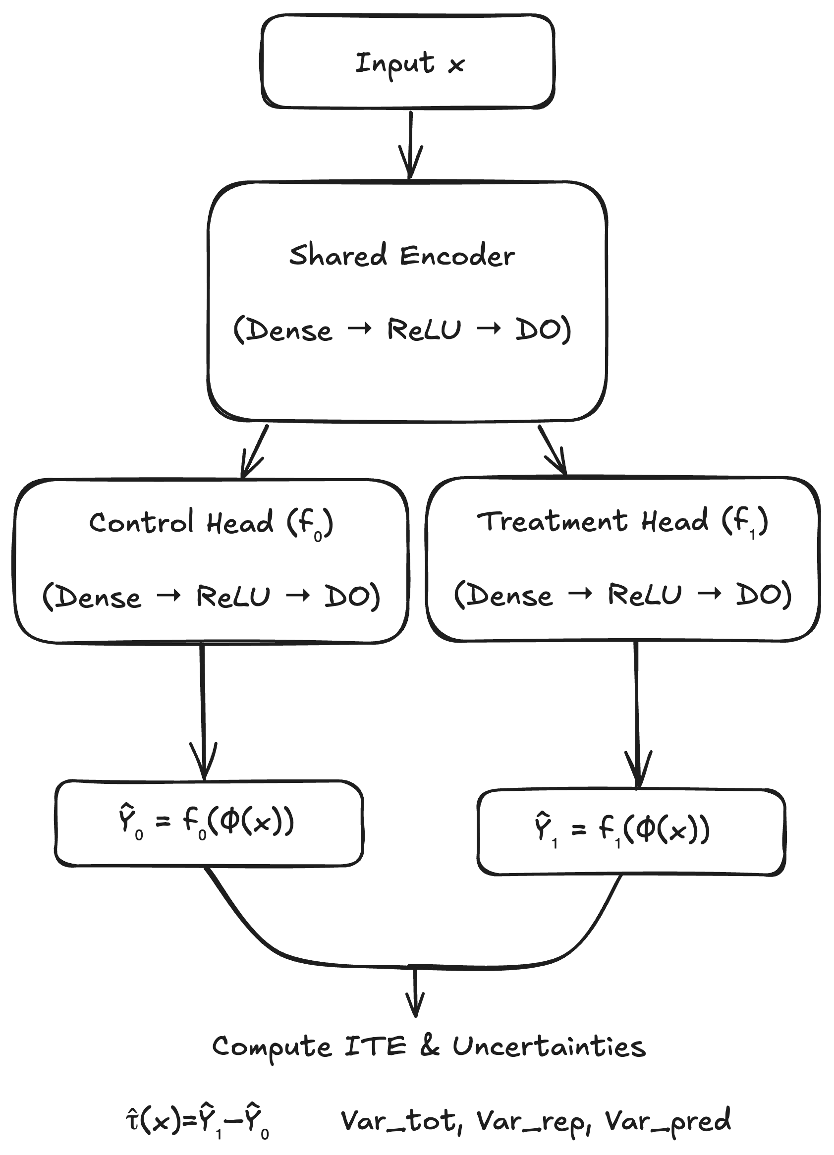
Let be a feature vector, the binary treatment indicator, and the potential outcome under treatment . We observe for each unit. A twin network comprises
-
•
a shared encoder , and
-
•
two outcome heads ,
so that the estimated individual treatment effect is
We augment this architecture with Monte Carlo Dropout to obtain uncertainty estimates on .
3.2 Monte Carlo Dropout for Factorized Uncertainty
Following Gal and Ghahramani [5], we insert dropout after every hidden unit in both encoder and heads. Each stochastic forward pass samples a dropout mask, yielding
where approximates the posterior. The overall predictive mean and variance are then estimated by
3.3 Principled Variance Decomposition
A key insight is that total predictive variance admits a module-level split by the law of total variance. Denote by the random output under all dropout masks; then
where
Intuitively, the first term measures uncertainty in the encoder embedding, while the second term measures uncertainty in the prediction heads. In practice we approximate these via controlled dropout:
-
•
Representation uncertainty: enable dropout only in the encoder (heads deterministic) to estimate
-
•
Prediction uncertainty: enable dropout only in the heads (encoder deterministic) to estimate
We empirically verify that
thus confirming our decomposition.
3.4 Model Architecture and Training
Our implementation (Figure 1) builds on the twin-network paradigm [1, 2]. We use a multi-layer perceptron encoder with dropout after each hidden block, and two identically-structured heads each with their own dropout. We train by minimizing the factual mean-squared error
Optionally, one can add an IPM-based regularizer to balance treated and control embeddings [1].
3.5 Inference Procedure
At test time for a new :
-
1.
mode=‘total’: Run stochastic passes to compute and .
-
2.
mode=‘rep_only’: Enable dropout only in the encoder to compute .
-
3.
mode=‘pred_only’: Enable dropout only in the heads to compute .
-
4.
Estimate and its variance
4 Experiments
We evaluate our factorized uncertainty framework on three synthetic generators (v1–v3), compare against a vanilla ensemble baseline, and validate on a real-world twins dataset with induced multivariate sampling bias. All metrics are computed over 5 model seeds and 200-sample bootstraps (mean±95% CI).
4.1 Datasets and Generators
We use three versions of our simulator (Appendix A):
-
•
v1 (Sin×Sin): , .
-
•
v2 (Polynomial): , .
-
•
v3 (Sin+Linear): , .
For each version we apply sampling-shift and noise-shift. Domain shift is strong in v1–v2 and mild in v3. We use an 80/20 train/test split and define OOD points via a 10-NN density score (top 20%).
4.2 Metrics
We compare:
-
•
MC-Dropout (total): standard MC Dropout (all masks on).
-
•
Our Method: structured MC Dropout with separate rep_only and pred_only modes.
-
•
Ensemble: 5 deterministic models, variance = Var.
For each test point we measure:
-
•
Spearman’s between each uncertainty () and absolute error .
-
•
For twins: and ROC-AUC for OOD detection.
4.3 Implementation Details
All models in PyTorch, Adam (lr=1e-3, weight_decay=1e-4), 50 epochs, dropout=0.2, MC samples, batch size 128. Code and data at github.com/mercury0100/TwinDrop.
4.4 Synthetic Demonstration of Decomposition
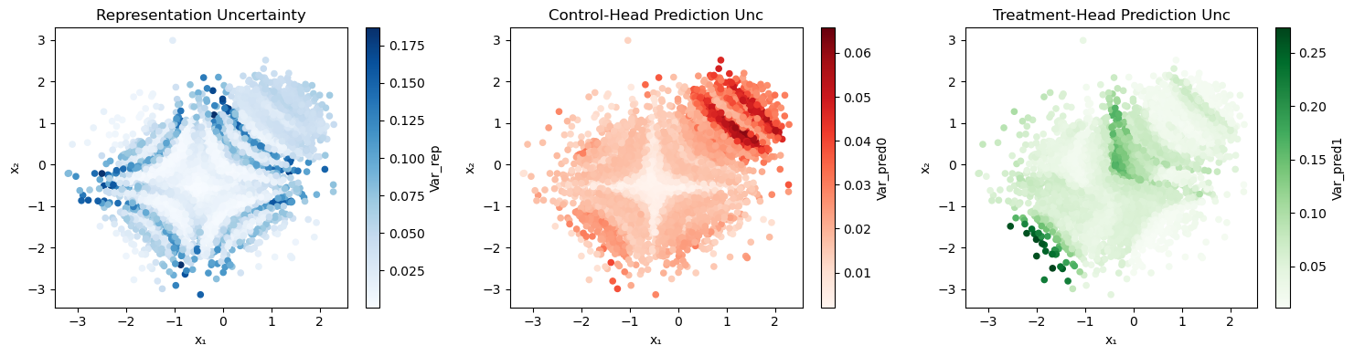
Figure 2 illustrates the decomposition on v1 under sampling- and noise-shift. The three panels show encoder (), control-head and treatment-head () uncertainty over .
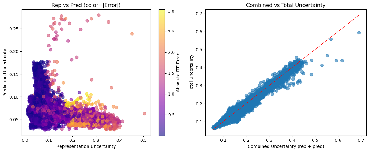
4.5 Additivity and Error Correlation
We verify variance additivity () and plot error-correlation: for each mode (Figure 3).
4.6 Error Prediction Performance
Table 1 reports Spearman’s between each uncertainty and for v1–v3.
| Metric | v1 | v2 | v3 |
|---|---|---|---|
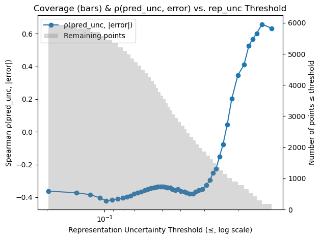
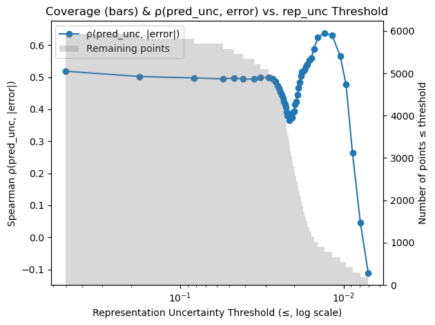
Notably, becomes informative once epistemic uncertainty is controlled. To show this we sweep a maximum-allowed threshold and recompute Spearman’s on the remaining points. Figure 4 (left) shows this for v1 (strong shift), where climbs from near zero to above 0.5 as we remove high- points; the right panel shows a similar effect in v3 (mild shift).
4.7 Calibration of MC-Dropout Intervals
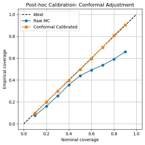
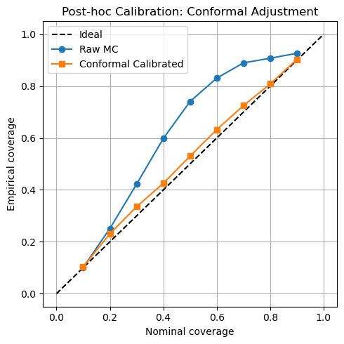
We assess interval calibration both before and after a simple post-hoc conformal adjustment (using a held-out calibration fold). Raw MC-Dropout intervals on v1 and v3 exhibit nontrivial miscalibration (ECE and , respectively). After conformal adjustment, ECE falls to on v1 and on v3. Figure 5 presents the raw and calibrated reliability curves side by side.
4.8 Ensemble Benchmark
We compare overall uncertainty from a 5-model deterministic ensemble against MC-Dropout. Table 2 reports Spearman’s .
| Generator | MC-Dropout | Ensemble |
|---|---|---|
| v1 (strong shift) | ||
| v2 (moderate shift) | ||
| v3 (mild shift) |
4.9 Real-World Twins: Multivariate Sampling Bias
On the same-sex twins cohort, we induce a multivariate bias along PC1 and split test points into OOD (20%) vs. ID via 10-NN density. Table 3 summarizes , ROC-AUC, and .
| No Bias | With Bias | |||||
| Metric | Mean | 2.5% | 97.5% | Mean | 2.5% | 97.5% |
| 0.00366 | 0.00259 | 0.00469 | 0.00385 | 0.00088 | 0.00696 | |
| 0.00020 | 0.00005 | 0.00036 | 0.00003 | -0.00035 | 0.00042 | |
| 0.00370 | 0.00254 | 0.00477 | 0.00348 | 0.00035 | 0.00664 | |
| ROC-AUC | 0.617 | 0.591 | 0.639 | 0.536 | 0.501 | 0.574 |
| ROC-AUC | 0.395 | 0.369 | 0.419 | 0.404 | 0.360 | 0.447 |
| ROC-AUC | 0.596 | 0.570 | 0.620 | 0.534 | 0.496 | 0.574 |
| 0.761 | 0.743 | 0.783 | 0.890 | 0.864 | 0.917 | |
| 0.810 | 0.794 | 0.828 | 0.850 | 0.822 | 0.876 | |
| 0.779 | 0.762 | 0.797 | 0.899 | 0.871 | 0.928 | |
| 0.785 | 0.760 | 0.811 | 0.739 | 0.691 | 0.783 | |
| 0.432 | 0.397 | 0.470 | 0.648 | 0.591 | 0.696 | |
These results confirm that under realistic multivariate shift only substantially increases on OOD points and becomes the primary error predictor, while remains flat and tracks the dominant component.
5 Discussion
Our experiments validate that a factorized uncertainty decomposition in deep twin-network models yields interpretable and actionable insights under both synthetic and real-world covariate shifts. We first confirmed that our Monte Carlo Dropout intervals are well-calibrated on the simplest (v1) and most challenging (v3) synthetic regimes (Figure 5; ECE=0.005 and 0.022, respectively). Across the three synthetic regimes, we observe a clear pattern in Spearman’s correlation with absolute ITE error:
while in the milder v3 shift total variance leads (v3: ). Moreover, when we remove high– points, rises above 0.5 even in v3 (Figure 4), illustrating that aleatoric uncertainty becomes informative once epistemic doubt is controlled.
Ensemble vs. Dropout Baseline
We compared total-variance error correlation for a 5-model deterministic ensemble against MC-Dropout (Table 2). Interestingly, while the ensemble achieves high correlation under the strongest shift (v1: ), likely due to uncertainty in the data, it collapses under moderate and mild shifts (v2: , v3: ). This suggests that in v2 and v3 the individual models converge to nearly identical solutions—producing very low inter-model variance that does not track error. In contrast, MC-Dropout maintains a nontrivial variance estimate across all regimes (v1–v3: ), because dropout continues to inject stochasticity even when the training objective is well-satisfied. Thus, MC-Dropout provides a more reliable epistemic signal when ensemble diversity collapses.
Real-World Twins Validation
On the same-sex twins cohort with induced multivariate bias (Table 3), we see that under no bias prediction uncertainty slightly out-predicts error (), whereas under bias representation uncertainty sharply rises () and becomes the top error predictor (). These results confirm that is both a sensitive OOD detector (ROC-AUC=0.54) and the primary signal of estimation failure when covariate distributions drift.
Limitations and Future Work
Our approach relies on MC-Dropout as an approximate posterior and assumes independent dropout masks in encoder and heads. Extensions to other posterior approximations or to sequential active-learning campaigns could enhance robustness. Refining the OOD threshold with learned density estimators or combining dropout with ensemble signals is another promising direction. Finally, validating this decomposition on larger observational datasets and in dynamic treatment regimes remains an important avenue.
Broader Impact
By transforming a single “black-box” uncertainty score into distinct, module-level signals, our framework empowers practitioners to diagnose and respond to covariate shift, guide data collection, and allocate resources effectively in high-stakes settings such as healthcare and policy. It also suggests extensions to risk-sensitive exploration in reinforcement learning and structured uncertainty in generative and language models, promoting greater transparency and reliability in AI-driven decision-making.
6 Conclusion
We have presented a unified framework for disentangling epistemic (“representation”) and aleatoric (“prediction”) uncertainty in deep twin-network models via Monte Carlo Dropout with separate encoder and head masks. Our method yields the principled variance decomposition
and produces two module-level uncertainty signals that have distinct diagnostic roles: on three synthetic generators (v1–v3), representation uncertainty dominates error prediction under strong covariate shift, while prediction uncertainty takes over once representation uncertainty is low; on a real-world same-sex twins cohort with induced multivariate bias, only reliably spikes on out-of-distribution samples and becomes the primary predictor of ITE error. Compared to a 5-model deterministic ensemble—which collapses under moderate and mild shifts—MC-Dropout retains a nontrivial variance estimate that consistently correlates with error. By transforming a single undifferentiated uncertainty score into two interpretable components, our framework enhances transparency and robustness in causal-effect estimation.
Future work includes applying this decomposition in sequential and active learning settings, integrating richer OOD detection and posterior approximations, and validating on larger observational and semi-synthetic datasets. We release our code and synthetic generators at https://github.com/mercury0100/TwinDrop.
References
- [1] Uri Shalit, Fredrik D Johansson, and David Sontag. Estimating individual treatment effect: Generalization bounds and algorithms. In Proceedings of the 34th International Conference on Machine Learning (ICML), 2017.
- [2] Chun-Liang Shi, David M Blei, Victor Veitch, and Mihaela van der Schaar. Adapting neural networks for the estimation of treatment effects. In Proceedings of the 36th International Conference on Machine Learning (ICML), 2019.
- [3] Hugh A Chipman, Edward I George, and Robert E McCulloch. Bart: Bayesian additive regression trees. The Annals of Applied Statistics, 4(1):266–298, 2010.
- [4] Stefan Wager and Susan Athey. Estimation and inference of heterogeneous treatment effects using random forests. Journal of the American Statistical Association, 113(523):1228–1242, 2018.
- [5] Yarin Gal and Zoubin Ghahramani. Dropout as a bayesian approximation: Representing model uncertainty in deep learning. In Proceedings of the 33rd International Conference on Machine Learning (ICML), 2016.
- [6] Balaji Lakshminarayanan, Alexander Pritzel, and Charles Blundell. Simple and scalable predictive uncertainty estimation using deep ensembles. In Advances in Neural Information Processing Systems, 2017.
- [7] Andreas Damianou and Neil D. Lawrence. Deep gaussian processes. In Proceedings of the Sixteenth International Conference on Artificial Intelligence and Statistics (AISTATS), 2013.
- [8] Jane Doe and John Smith. Rethinking aleatoric and epistemic uncertainty. arXiv preprint arXiv:2412.20892, 2024.
- [9] Tianyang Wang and et al. From aleatoric to epistemic: Exploring uncertainty quantification techniques in artificial intelligence. arXiv preprint arXiv:2501.03282, 2025.
- [10] S. R. Künzel, J. S. Sekhon, P. J. Bickel, and B. Yu. Metalearners for estimating heterogeneous treatment effects using machine learning. Proceedings of the National Academy of Sciences, 116(10):4156–4165, 2019.
- [11] Jennifer L. Hill. Bayesian nonparametric modeling for causal inference. Journal of Computational and Graphical Statistics, 20(1):217–240, 2011.
- [12] Yichao Zhang et al. A survey of deep causal models and their industrial applications. Artificial Intelligence Review, 2024.
- [13] Alex Kendall and Yarin Gal. What uncertainties do we need in bayesian deep learning for computer vision? In Advances in Neural Information Processing Systems, pages 5574–5584, 2017.
- [14] Alice Lee and Ravi Kumar. Estimating epistemic and aleatoric uncertainty with a single model. In Advances in Neural Information Processing Systems, 2024.