Dispersion interactions between semiconducting wires
Abstract
The dispersion energy between extended molecular chains (or equivalently infinite wires) with non-zero band gaps is generally assumed to be expressible as a pair-wise sum of atom-atom terms which decay as . Using a model system of two parallel wires with a variable band gap, we show that this is not the case. The dispersion interaction scales as for large interwire separations , as expected for an insulator, but as the band gap decreases the interaction is greatly enhanced; while at shorter (but non-overlapping) separations it approaches a power-law scaling given by , i.e. the dispersion interaction expected between metallic wires. We demonstrate that these effects can be understood from the increasing length scale of the plasmon modes (charge fluctuations), and their increasing contribution to the molecular dipole polarizability and the dispersion interaction, as the band gaps are reduced. This result calls into question methods which invoke locality assumptions in deriving dispersion interactions between extended small-gap systems.
pacs:
34.20.Gj 73.22.-f 31.15.apI Introduction
Conventionally, the dispersion interaction between two systems is formulated in terms of correlated fluctuations described by local (frequency-dependent) polarizabilities which gives rise to the familiar atom–atom interaction at leading order Stone (1996). This form of the interaction has been used with a good measure of success in studies of many systems, from gases to solids, including complexes of biological molecules and organic molecules. These are typically insulators; that is, they have large HOMO–LUMO gaps.
It has been known for a very long time that the additive atom–atom form of the dispersion does not hold very well for metallic systems. The classic case of an atom interacting with a thin metallic surface shows deviations from the additive law: the correct treatment of the metal results in a power law Casimir and Polder (1948), but summing over atom–atom terms leads to a interaction. More recently, strong deviations from additivity have been demonstrated in the interactions of extended systems of metals or zero band-gap materials with at least one nano-scale dimension Dobson (2007); Dobson et al. (2006, 2001, 2004); Drummond and Needs (2007).
The semi-classical picture is useful for understanding the source of the differences in the metallic and insulating cases. In an insulator, electronic perturbations decay exponentially with distance. We can therefore treat electron correlations as being local. At lowest order, these local fluctuations give rise to instantaneous local dipoles, and the correlation between these local dipoles gives rise to the atom–atom interaction. However, in a zero band-gap material, electronic fluctuations are long-ranged, particularly if one or two of the dimensions are nano-scale Dobson (2007). It is these long-ranged fluctuations that give rise to the non-additivity of the dispersion and deviations from the atom–atom interaction.
While the insulating and metallic cases are now well understood, little is known of the intermediate, semi-conducting case. The nature of the dispersion interaction between extended molecules with finite but small HOMO–LUMO gaps less than about 0.2 a.u. (5 eV) remains an open question. A large number of important nano-molecules fall into this category, such as carbon nano-tubes and the ‘lander’-type molecules that are used as organic conductors. The electronic structure of materials made of these molecules depends strongly on structures they assume in the bulk, often via self-assembly. Consequently it is very important to understand exactly how these molecules interact. The dispersion interaction is the dominant source of attraction between these -conjugated systems. For want of a clearer understanding, many studies assume the usual insulating case for the atom–atom form of this interaction. As we shall show in this article, this is both qualitatively and quantitatively incorrect for semiconducting molecules.
A word of clarification: we use the term ‘non-additive’ here to describe deviations from the additive atom-atom picture of the dispersion interaction between two molecules. It is also commonly used to refer to the deviation from pair additivity seen in the interactions of three or more distinct molecules, but we are not concerned with such effects here, except for a brief comment in the Discussion.
II Interacting wires using Hückel (Tight-binding) theory
The dispersion energy appears at second-order in intermolecular perturbation theory and is formally expressed in terms of the exact eigenstates and eigenenergies of the non-interacting systems Stone (1996). In a mean-field theory the dispersion energy between two subsystems ( and ), can be expressed as a sum over the single-electron wavefunctions localised to each subsystem:
| (1) |
where () are occupied (virtual) single-particle wavefunctions in either subsystem or , and is the eigenvalue of the -th wavefunction. Assuming two parallel wires, aligned parallel to the axis and separated by a distance , the integral which appears above has the form:
| (2) |
and is the Coulomb interaction between the charge density due to excitation in subsystem with in .
In periodic systems, the wavefunction can be expressed in Bloch form, i.e. , and so the co-density can have a long-wavelength modulation, whose electrostatic field will not be well described by a multipole expansion at separations comparable to this length scale. Furthermore, in small-gap systems, these excitations have plasmon character and contribute significantly to , as we discuss below.
Hückel (tight-binding) theory gives us a convenient formalism for evaluating the above expression for interactions between two one-dimensional wires. We considered a two-band model Hamiltonian of the form
| (3) |
where are alternating bond-strengths between adjacent sites, as would be encountered in a chain of (H2)n or a -conjugated polyene. We computed the interactions between two such parallel wires, each consisting of identical atoms, equally spaced at intervals of , such that the unit cell is of length and contains two atoms. Assuming periodic boundary conditions over a crystal cell of length , then there are two bands per wavevector. The single-particle wavefunctions and energies of sych a system can be found analytically. The band structure is given by
| (4) |
and the set of wavevectors by
| (5) |
corresponds to a uniform wire with energy eigenvalues given by , which in the limit of large has a vanishing band-gap at half-filling (i.e. is a metal). The opposite limit () corresponds to a chain of isolated dimers with energy eigenvalues , independent of wavevector, and corresponds to the perfect insulator. By varying the ratio between 0 and 1, we can very conveniently probe the dispersion interaction in the intermediate (semiconducting) regime, with the band-gap given by . The required integrals can be evaluated Spencer (2009) as:
| (6) |
where are reciprocal lattice vectors of the primitive unit cell and is the (analytic) Fourier transform of obtained by assuming highly-localised basis functions on each atom. is the zero-th order modified Bessel function of the second kind and is the Fourier transform of the potential generated by a one-dimensional lattice at a field point at from the latticeEpstein (1903, 1906); Tosi (1964). decays exponentially with increasingly large arguments and so typically only the 10 smallest reciprocal lattice vectors need to be included in the summation in order to obtain converged results.
The calculations presented here use 8401 Monkhorst-Pack -points to sample the Brillouin zone, which corresponds in real-space to wires consisting of 16802 sites per crystal cell. Such fine k-point sampling was required to obtained converged results with respect to system size.
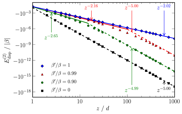
As shown in fig. 1, the dispersion interaction between two uniform wires () varies as across the whole range of , in good agreement with previously obtained results via RPADobson (2007) and QMCDrummond and Needs (2007) for metallic wires. The interaction between chains of isolated dimers () varies as , as would be expected from the conventional picture of dispersion interactions. In the semiconducting regime, there is no unique exponent which characterises the dispersion interaction over all . However, at small separations , it tends to the metallic behaviour (), whereas large it tends to insulating behaviour .
III Interacting H2 chains using SAPT(DFT)
The principal drawback of the Hückel model is the lack of electron correlation, and hence screening, within each subsystem. For more realistic calculations we can use the symmetry-adapted perturbation theory based on density-functional theory Misquitta et al. (2003); Hesselmann et al. (2005); Misquitta et al. (2005) (SAPT(DFT)), where the dispersion energy is evaluated not via a sum-over-states but through a coupled Kohn–Sham formulation based on the density response functions of the interacting moleculesLonguet-Higgins (1965):
| (7) |
where are the frequency-dependent density response functions of the molecules which describe the propagation of a frequency-dependent perturbation in a molecule, from one point to another, within linear-response theory. The second-order dispersion energy is exact in this formulation if exchange effects are neglected.
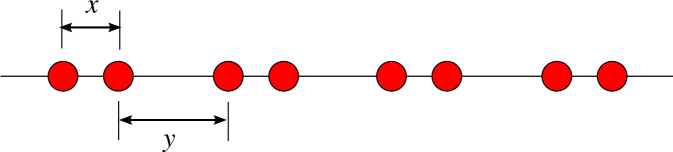
We have studied the interactions between two parallel finite (H2)n (fig. 2) chains with and and distortion parameters and , where is the ratio of the alternate bond lengths. The HOMO-LUMO gap of a hydrogen chain can be modified by simply introducing a difference in alternate bond lengths. The distortion parameter gives us a convenient way to control the electronic structure of the chain and allows us to study the interactions between insulating, semiconducting and (near) metallic chains in one framework.
The frequency-dependent density response functions that appear in eq. (7) were evaluated with coupled Kohn–Sham perturbation theory, using the PBE0 functional with a hybrid kernel consisting of 75% adiabatic LDA and 25% coupled Hartree-Fock. The accuracy of this approach for the dispersion energy of small molecules surpasses that of Møller-Plesset perturbation theory and rivals that of coupled-cluster methods Misquitta et al. (2005); Hesselmann and Jansen (2003); Hesselmann et al. (2005); Podeszwa and Szalewicz (2005). Furthermore, there is no qualitative change in our results when the fraction of HF exchange is increased, so the results presented here are unlikely to be artifacts of the shortcomings of coupled Kohn–Sham perturbation theory Champagne et al. (1998); Sekino et al. (2007). All calculations used the cc-pVDZ basis which will result in a significant underestimation of the strength of the contribution to the dispersion energy that arises from transverse polarization, but should better describe the contribution arising from the longitudinal polarization. Since it is the longitudinal polarization that is most important in these systems, we expect our results to be qualitatively correct.
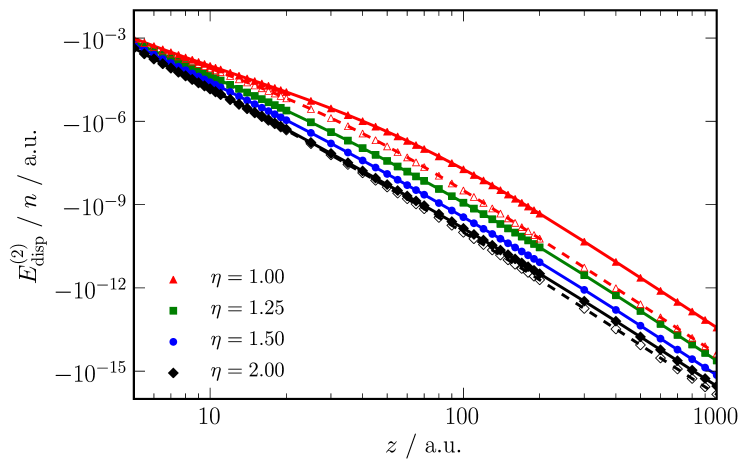
Dispersion energies are displayed in fig. 3 and the effective power laws for the physically important separations between 6 and 20 a.u. are shown in table 1 together with HOMO–LUMO gaps. For insulating chains with an additive dispersion interaction we would expect two regimes determined by chain length : for we should expect the infinite chain result, i.e., the effective dispersion interaction should decay as , and for we should recover the usual power law. This is what we see with the chains with the largest distortion parameter, , which exhibit large HOMO–LUMO gaps. As the distortion parameter approaches unity and the HOMO–LUMO gap consequently decreases, the deviation from the additive insulating case becomes increasingly apparent, and for the longest of the chains considered here the dispersion interaction is significantly enhanced. For example at a.u. (roughly half the chain length) an chain has a dispersion interaction two orders of magnitude larger than an chain. Additionally, we see increasing finite-size effects: the power laws for the and chains, which were very similar for , are considerably different for .
| (H2)16 | (H2)32 | |||
|---|---|---|---|---|
| 2.0 | 0.370 | 4.89 | 0.366 | 4.84 |
| 1.5 | 0.280 | 4.58 | 0.270 | 4.50 |
| 1.25 | 0.202 | 4.20 | 0.183 | 4.09 |
| 1.0 | 0.099 | 3.52 | 0.057 | 3.17 |
IV Multipole expansion
We can understand these effects in terms of the multipole expansion. The multipole form of the dispersion energy is usually formulated in terms of (local) atomic polarizabilities. This leads to the usual atom–atom interaction (at leading order) and would not account for the anomalous dispersion power laws that we have observed in the chains. However the complete distributed-polarizability description is non-local: that is, it describes the change in multipole moments at one atom in response to a change in electrostatic fields at another.
We obtain the multipole form of eq. (7) by expanding the Coulomb terms using the distributed form of the multipole expansion where and denote (atomic) sites and and are multipole indices — 00 for the charge, 10, and for the components of the dipole, and so on. is the multipole moment operator for moment of site and are the interaction tensors that contain the distance and angular dependence (see Ref.Stone (1996) for details). Inserting this expansion in eq. (7) we obtain the multipole form for the dispersion energy:
| (8) |
Here is the interaction function between multipole on site in subsystem and multipole on site in , while are the frequency-dependent non-local polarizabilities for sites and , and may be expressed in terms of the frequency-dependent density susceptibility asMisquitta and Stone (2006)
| (9) |
There are no assumptions made in deriving eq. (8), other than that spheres enclosing the atomic charge densities on different molecules do not overlap. We have calculated distributed polarizabilities using the constrained density-fitting algorithm Misquitta and Stone (2006).
Eq. (8) involves a quadruple sum over sites and is therefore computationally demanding. To reduce this cost, we normally make a simplification by localizing the non-local polarizabilities. That is, the non-local polarizabilities — the with — are transformed onto one or other site using the multipole expansion Le Sueur and Stone (1994); Lillestolen and Wheatley (2007). This transformation is possible only if the non-local terms decay fast enough with inter-site distance. If not, the multipole expansion used in the transformation diverges and the localization is no longer possible. As we shall see, this is precisely what happens in the (H2)n chains as the distortion parameter decreases.
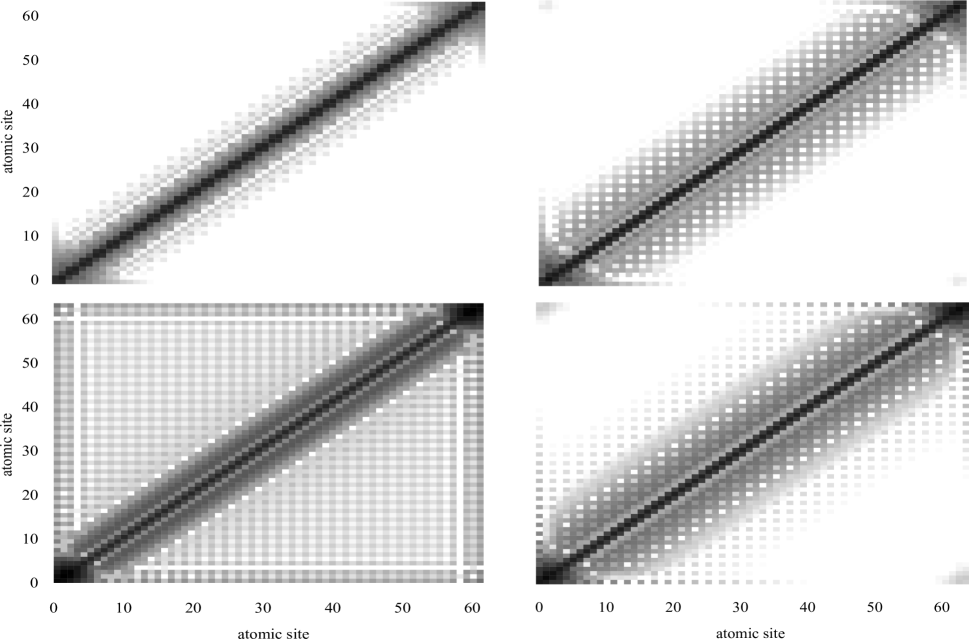
An important feature of the non-local polarizability description is the presence of charge-flow polarizabilities—terms with or that describe the flow of charge in a molecule—which are usually small and die off quickly with distance. The lowest rank charge-flow polarizability is : if is the potential at site , the change in charge at site is given by . For a system with a large HOMO–LUMO gap the charge-flow terms are expected to be short-range. The charge-flow polarizabilities of the (H2)32 chain with can be empirically modelled reasonably well with an exponential, that is,
| (10) |
where is the intersite distance and a.u. In this case, the charge-flow polarizabilities drop by more than an order of magnitude within a few bonds. This is illustrated in fig. 4. However, as we reduce the distortion parameter the charge-flow polarizabilities decay more and more slowly with site-site distance, until, at , they span the entire length of the chain. Even for the chain, these non-local charge-flow polarizabilities can no longer be localized without incurring a significant error, but for the chains with and localization results in a qualitatively incorrect physical picture.
Moreover the charge-flow polarizabilities contribute to the dipole–dipole polarizability in the direction of the chain, and this contribution increases dramatically as the band-gap decreases. For a 64-atom H chain with , the static dipole polarizability parallel to the chain, calculated as described above, is about 410 a.u., of which 180 a.u. is contributed by charge-flows. When , so that the H atoms are equally spaced, is about 11350 a.u., larger by about two orders of magnitude, and all of this increase is attributable to the charge-flow effects.
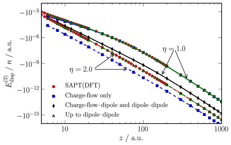
We have calculated the dispersion energy using eq. (8) with distributed polarizabilities, including terms to rank 1. Higher ranking terms can be included, but these are not needed for the hydrogen chains. These results are presented in fig. 5 for the (H2)32 chains with and . First of all, consider the insulating chain (): the charge-flow polarizabilities alone severely underestimate the dispersion energy, but when terms up to rank 1 are included the agreement of eq. (8) with the non-expanded SAPT(DFT) value for is excellent for all inter-chain separations shown in the figure. However, at , the dispersion interaction is entirely dominated by the pure charge-flow (i.e. ) terms, the higher order terms involving the dipole polarisabilities making a negligible contribution. Since the overall dispersion interaction is greatly enhanced as is reduced, this implies that these pure charge-flow terms enhance the dispersion interaction in this limit.
Why do the charge-flow terms result in the anomalous power laws? The lowest rank charge-flow terms, , that appear in eq. (8) are associated with -functions for the charge-charge interaction: , where is the distance between site on one wire and site on the other. If the wires are separated by distance vector and and are distance vectors for sites and along the chains then . The dispersion energy arising from just the charge-flow terms is
| (11) |
In contrast to the dipole-dipole polarizabilities, the charge-flow polarizabilities satisfy the sum-rule , which is a direct consequence of the charge conservation requirement: . This leads to cancellation between the charge-flow contributions to the total dispersion energy, and to an distance dependence at long range, but the cancellation is incomplete at short range, and terms in also occur. To see how this arises, consider the following length scales: (1) , which is a measure of the extent of the charge fluctuations determined by the exponential decay of the charge-flow polarizabilities assumed in eq. (10), and (2) , the chain length.
- •
-
•
: In this region the extent of the charge fluctuations is small compared with and only those close to are important. We can therefore expand about using the multipole expansion. The leading term in this expansion is
(12) where we have used the charge-flow sum rule. So we see that the contributions sum to zero in this region. However, the higher-order contributions are non-zero.
-
•
: In this limit both and can be expanded in a multipole expansion about : , and likewise for . Once again, the leading terms vanish because of the sum rule, leaving only the effective dipole-dipole contribution:
(13) This explains the large- charge-flow contribution to the dispersion energy shown in fig. 5. Notice that for the near-metallic wires, this contribution to the total molecular coefficient dominates that from the dipole-dipole polarizabilities, but for the large-gap wires the opposite is true.
In short, the charge-flow polarizabilities give rise to the changes in power-law of the dispersion energy and also contribute to an enhancement of the effective coefficient, applicable at long range.
V Discussion
The physical picture which emerges from both the Hückel approach and the ab initio calculations is the following.
-
•
In systems with a finite but small gap, spontaneous charge-fluctuations (plasmon modes in the infinite case) introduce a secondary length-scale intermediate in size to the interatomic distance and the system size. This length scale grows as the gap gets smaller.
-
•
For separations small compared with this length scale, the dispersion energy arising from the correlated fluctuations has metallic character.
-
•
At that are large compared with the length scale of the fluctuations, the dispersion can be described using London’s dipole approximation, giving behaviour, but the magnitude of the fluctuations now depends strongly on the band gap, leading to orders of magnitude enhancement over the insulator case.
-
•
In small-gap systems these fluctuations give rise to a strong non-additivity in the polarizability. For example, the ratio of the longitudinal static polarizabilities for the near-metallic and insulating (H2)32 chains is 28. The dispersion energy is proportional to the square of the polarizability, that is, 784. This is roughly the ratio of the dispersion energies for these two cases but only at separations much greater than the chain length. Any attempt to extrapolate this result to shorter distances results in a severe overestimation of the dispersion energy.
-
•
This effect is not a consequence of retardation (we use the non-relativistic Hamiltonian) or damping (charge-density overlap is negligible). It originates from the complex behaviour of the non-local charge-flow polarizabilities. These are terms of rank zero that describe charge fluctuations in the system and are associated with a delocalized exchange-correlation hole Angyan (2007, 2009). This delocalization can be quantified using the localization tensor Resta and Sorella (1999); Angyan (2009) and may give us a quantitative method for defining the charge fluctuation length-scale, . We are currently investigating this possibility.
-
•
We have demonstrated that both the change in power-law with distance and the enhancement of the dispersion energy can be understood using non-local polarizability models containing charge-flow polarizabilities.
-
•
It should come as no surprise that these effects are also strongly dependent on system size (see fig.3).
These results call into question theoretical methods that impose locality so as to scale linearly with system size (LCCSD(T), LMP2), or that approximate the dispersion energy using a pair-wise interaction, as is done with dispersion-corrected DFT methods and empirical potentials. In the former, these effects can be included by extending the region of locality, though at the cost of losing linearity in scaling, but the latter methods should not be applied to systems such as these. Even DFT functionals with a non-local dispersion correction, such as the van der Waals functional of Dion et al.Dion et al. (2004) and the more recent functional of Vydrov and Van Voorhis Vydrov and Voorhis (2009) are unlikely to contain the correct physics because of an implicit assumption of locality in the polarizability. These functionals will include many-body non-additive effects between non-overlapping systems, but not the non-additive effects within each system such as those described here. On the other hand, methods based on the random phase approximation and quantum Monte Carlo should be able to describe the non-additive effects described in this paper if finite-size effects are kept under control.
In systems containing carbon atoms, such as -conjugated chains, the contributions from the core electrons will at least partially mask those from the more mobile electrons, so it is possible that the changes in power-law of the dispersion interaction will not be as dramatic as those we see in the (H2)n chains. But we should nevertheless expect a high degree of non-additivity arising from the charge-flow terms. One indicator of this non-additivity is the non-linear dependence of the molecular polarizability on system size. This has been already demonstrated above and is further supported by the experimental work of Compagnon et al. Compagnon et al. (2001) on the polarizabilities of the fullerenes C70 and C60 which are found to be in the ratio 1.33 rather than the ratio that would be expected if the systems were additive. Therefore, if reliable -models are to be constructed for extended -conjugated systems, these models will need to absorb the effects of the non-additivity of the charge-flow polarizabilities. That is, they should be tailored to suit the electronic structure of the system rather than be transferred from calculations on smaller systems. The Williams–Stone–Misquitta (WSM) procedure Misquitta and Stone (2008a); Misquitta et al. (2008); Misquitta and Stone (2008b) is one such method that is capable of constructing effective local polarizability and dispersion models that account for the electronic structure of the system. In fact, the non-local models presented in this paper are derived in the first step of the WSM procedure. We are currently investigating the behaviour of WSM dispersion models for a variety of carbon systems.
Finally, strongly delocalized systems will also have important contributions to the dispersion energy from terms of third order in the interaction operator, that is, from the hyperpolarizabilities. We have not considered such terms in this paper. Furthermore, in ensembles of such systems there will be strong non-additive effects between molecules. We are currently investigating the nature and importance of this type of non-additivity.
VI Acknowledgements
We thank University College London for computational resources. AJM and JS thank EPSRC for funding.
References
- Stone (1996) A. J. Stone, The Theory of Intermolecular Forces (Clarendon Press, Oxford, 1996).
- Casimir and Polder (1948) H. B. G. Casimir and D. Polder, Phys. Rev. 73, 360 (1948).
- Dobson (2007) J. F. Dobson, Surface Science 601, 5667 (2007).
- Dobson et al. (2006) J. F. Dobson, A. White, and A. Rubio, Phys. Rev. Lett. 96, 073201(4) (2006).
- Dobson et al. (2001) J. F. Dobson, K. McLennan, A. Rubio, J. Wang, T. Gould, H. M. Le, and B. P. Dinte, Aust. J. Chem. 54, 513 (2001).
- Dobson et al. (2004) J. F. Dobson, J. Wang, B. P. Dinte, K. McLennan, and H. M. Le, Int. J. Quantum Chem. 101, 579 (2004).
- Drummond and Needs (2007) N. D. Drummond and R. J. Needs, Phys. Rev. Lett. 99, 166401(4) (2007).
- Spencer (2009) J. Spencer, Ph.D. thesis, University of Cambridge (2009).
- Epstein (1903) P. Epstein, Mathematische Annalen 56, 615 (1903).
- Epstein (1906) P. Epstein, Mathematische Annalen 63, 205 (1906).
- Tosi (1964) M. P. Tosi, Cohesion of ionic solids in the Born model (Academic Press, 1964), vol. XVI of Solid State Physics.
- Misquitta et al. (2003) A. J. Misquitta, B. Jeziorski, and K. Szalewicz, Phys. Rev. Lett. 91, 33201 (2003).
- Hesselmann et al. (2005) A. Hesselmann, G. Jansen, and M. Schutz, J. Chem. Phys. 122, 014103 (2005).
- Misquitta et al. (2005) A. J. Misquitta, R. Podeszwa, B. Jeziorski, and K. Szalewicz, J. Chem. Phys. 123, 214103 (2005).
- Longuet-Higgins (1965) H. C. Longuet-Higgins, Disc. Farad. Soc. 40, 7 (1965).
- Hesselmann and Jansen (2003) A. Hesselmann and G. Jansen, Phys. Chem. Chem. Phys. 5, 5010 (2003).
- Podeszwa and Szalewicz (2005) R. Podeszwa and K. Szalewicz, Chem. Phys. Lett. 412, 488 (2005).
- Champagne et al. (1998) B. Champagne, E. A. Perpete, S. J. A. van Gisbergen, E.-J. Baerends, J. G. Snijders, C. Soubra-Ghaoui, K. A. Robins, and B. Kirtman, J. Chem. Phys. 109, 10489 (1998).
- Sekino et al. (2007) H. Sekino, Y. Maeda, M. Kamiya, and K. Hirao, J. Chem. Phys. 126, 014107 (2007).
- Misquitta and Stone (2006) A. J. Misquitta and A. J. Stone, J. Chem. Phys. 124, 024111 (2006).
- Le Sueur and Stone (1994) C. R. Le Sueur and A. J. Stone, Mol. Phys. 83, 293 (1994).
- Lillestolen and Wheatley (2007) T. C. Lillestolen and R. J. Wheatley, J. Phys. Chem. A 111, 11141 (2007).
- Angyan (2007) J. G. Angyan, J. Chem. Phys. 127, 024108 (2007).
- Angyan (2009) J. G. Angyan, Int. J. Quantum Chem. 109, 2340 (2009).
- Resta and Sorella (1999) R. Resta and S. Sorella, Phys. Rev. Lett. 82, 370 (1999).
- Dion et al. (2004) M. Dion, H. Rydberg, E. Schroder, D. C. Langreth, , and B. I. Lundqvist, Phys. Rev. Lett. 92, 246401 (2004).
- Vydrov and Voorhis (2009) O. A. Vydrov and T. V. Voorhis, Phys. Rev. Lett. 103, 063004 (2009).
- Compagnon et al. (2001) I. Compagnon, R. Antoine, M. Broyer, P. Dugourd, J. Lerme, and D. Rayane, Phys. Rev. A 64, 025201 (2001).
- Misquitta and Stone (2008a) A. J. Misquitta and A. J. Stone, J. Chem. Theory Comput. 4, 7 (2008a).
- Misquitta et al. (2008) A. J. Misquitta, A. J. Stone, and S. L. Price, J. Chem. Theory Comput. 4, 19 (2008).
- Misquitta and Stone (2008b) A. J. Misquitta and A. J. Stone, Mol. Phys. 106, 1631 (2008b).