Dispersive hydrodynamics of soliton condensates for the Korteweg-de Vries equation
Abstract
We consider large-scale dynamics of non-equilibrium dense soliton gas for the Korteweg-de Vries (KdV) equation in the special “condensate” limit. We prove that in this limit the integro-differential kinetic equation for the spectral density of states reduces to the -phase KdV-Whitham modulation equations derived by Flaschka, Forest and McLaughlin (1980) and Lax and Levermore (1983). We consider Riemann problems for soliton condensates and construct explicit solutions of the kinetic equation describing generalized rarefaction and dispersive shock waves. We then present numerical results for “diluted” soliton condensates exhibiting rich incoherent behaviours associated with integrable turbulence.
1 Introduction
Solitons represent the fundamental localised solutions of integrable nonlinear dispersive equations such as the Korteweg-de Vries (KdV), nonlinear Schrödinger (NLS), sine-Gordon, Benjamin-Ono and other equations. Along with the remarkable localisation properties solitons exhibit particle-like elastic pairwise collisions accompanied by definite phase/position shifts. A comprehensive description of solitons and their interactions is achieved within the inverse scattering transform (IST) method framework, where each soliton is characterised by a certain spectral parameter related to the soliton’s amplitude, and the phase related to its position (for the sake of definiteness we refer here to the properties of KdV solitons). Generally, integrable equations support -soliton solutions which can be viewed as nonlinear superpositions of solitons. Within the IST framework -soliton solution is characterised by a finite set of spectral and phase parameters completely determined by the initial conditions for the integrable PDE.
The particle-like properties of solitons suggest some natural questions pertaining to the realm of statistical mechanics, e.g. one can consider a soliton gas as an infinite ensemble of interacting solitons characterised by random spectral (amplitude) and phase distributions. The key question is to understand the emergent macroscopic dynamics (i.e. hydrodynamics or kinetics) of soliton gas given the properties of the elementary, “microscopic” two-soliton interactions. It is clear that, due to the presence of an infinite number of conserved quantities and the lack of thermalisation in integrable systems the properties of soliton gases will be very different compared to the properties of classical gases whose particle interactions are non-elastic. Invoking the wave aspect of the soliton’s dual identity, soliton gas can be viewed as a prominent example of integrable turbulence [1]. The pertinent questions arising in this connection are related to the determination of the parameters of the random nonlinear wave field in the soliton gas such as probability density function, autocorrelation function, power spectrum etc.
The IST-based phenomenological construction of a rarefied, or diluted, gas of KdV solitons was proposed in 1971 by V. Zakharov [2] who has formulated an approximate spectral kinetic equation for such a gas based on the properties of soliton collisions: the conservation of the soliton spectrum (isospectrality) and the accumulation of phase shifts in pairwise collisions that results in the modification of an effective average soliton’s velocity in the gas. Zakharov’s spectral kinetic equation was generalised in [3] to the case of a dense gas using the finite gap theory and the thermodynamic, infinite-genus, limit of the KdV-Whitham modulation equations [4]. The results of [3] were used in [5] for the formulation of a phenomenological construction of kinetic equations for dense soliton gases for integrable systems describing both unidirectional and bidirectional soliton propagation and including the focusing, defocusing and resonant NLS equations, as well as the Kaup-Boussinesq system for shallow-water waves [6]. The detailed spectral theory of soliton and breather gases for the focusing NLS equation has been developed in [7].
The spectral kinetic equation for a dense soliton gas represents a nonlinear integro-differential equation describing the evolution of the density of states (DOS)—the density function in the phase space , where is the spectral parameter in the Lax pair associated with the nonlinear integrable PDE,
| (1.1) |
Here is the velocity of a “free” soliton, and the integral term in the second equation represents the effective modification of the soliton velocity in the gas due to pairwise soliton collisions that are accompanied by the phase-shifts described by the kernel . Both and are system specific. In particular, for KdV and . The spectral support of the DOS is determined by initial conditions. We note that, while for the KdV equation, one can have for other equatons, e.g. the focusing NLS equation, see [7] . Equation (1.1) describes the DOS evolution in a dense soliton gas and represents a broad generalisation of Zakharov’s kinetic equation for rarefied gas [2]. The existence, uniqueness and properties of solutions to the “equation of state” (the integral equation in (1.1) for fixed ) for the focusing NLS and KdV equations were studied in [8].
The original spectral theory of the KdV soliton gas [3] has been developed under the assumption that the spectral support of the DOS is a fixed, simply-connected interval of ; without loss of generality one can assume . In [7], [8] this restriction has been removed by allowing the spectral support to be a union of disjoint intervals , termed here s-bands: , (, ). In this paper we introduce a further generalization of the existing theory by allowing the endpoints of the s-bands be functions of . We show that this generalization has profound implications for soliton gas dynamics, in particular, the kinetic equation implies certain nonlinear evolution of the endpoints of the s-bands. We determine this evolution for a special type of soliton gases, termed in [7] soliton condensates. Soliton condensate represents the “densest possible” gas whose DOS is uniquely defined by a given spectral support . The number of disjoint s-bands in determines the genus of the soliton condensate. We show that the evolution of ’s in a soliton condensate is governed by the -phase averaged KdV-Whitham modulation equations [4], also derived in the context of the semi-classical, zero-dispersion limit of the KdV equation [9].
We then consider the soliton condensate dynamics arising in the Riemann problem initiated by a rapid jump in the DOS. Our results suggest that in the condensate limit the KdV dynamics of soliton gas is almost everywhere equivalent to the (deterministic) generalised rarefaction waves (RWs) and generalized dispersive shock waves (DSWs) of the KdV equation. We prove this statement for the genus zero case and present a strong numerical evidence for genus one. Our results also suggest direct connection of the “deterministic KdV soliton gases” constructed in the recent paper [10] with modulated soliton condensates.
Our work puts classical results of integrable dispersive hydrodynamics (Flaschka-Forest-McLaughlin [4], Lax-Levermore [9], Gurevich-Pitaevskii [11]) in a broader context of the soliton gas theory. Namely, we show that the KdV-Whitham modulation equations describe the emergent hydrodynamic motion of a special soliton gas—a condensate—resulting from the accumulated effect of “microscopic” two-soliton interactions. This new interpretation of the Whitham equations is particularly pertinent in the context of generalized hydrodynamics, the emergent hydrodynamics of quantum and classical many-body systems [52]. The direct connection between the kinetic theory of KdV soliton gas and generalized hydrodynamics was established recently in [53] (see also [54] where the Whitham equations for the defocusing NLS equation were shown to arise in the semi-classical limit of the generalised hydrodynamics of the quantum Lieb-Liniger model).
Our work also paves the way to a major extension of the existing dispersive hydrodynamic theory by including the random aspect of soliton gases. To this end we consider “diluted” soliton condensates whose DOS has the same spectral distribution as in genuine condensates but allows for a wider spacing between solitons giving rise to rich incoherent dynamics associated with “integrable turbulence” [1]. In particular, we show numerically that evolution of initial discontinuities in diluted soliton condensates results in the development of incoherent oscillating rarefaction and dispersive shock waves.
An important aspect of our work is the numerical modelling of soliton condensates using -soliton KdV solutions with large configured according to the condensate density of states. The challenges of the numerical implementation of standard -soliton formulae for sufficiently large due to rapid accumulation of roundoff errors are known very well. Here we use the efficient algorithm developed in [45], which relies on the Darboux transformation. We improve this algorithm following the recent methodology developed in [46] for the focusing NLS equation with the implementation of high precision arithmetic routine. Our numerical simulations show excellent agreement with analytical predictions for the solutions of soliton condensate Riemann problems and provide a strong support to the basic conjecture about the connection of KdV soliton condensates with finite-gap potentials.
It should be noted that soliton condensates have been recently studied for the focusing NLS equation, where they represent incoherent wave fields exhibiting distinct statistical properties. In particular, it was shown in [55] that the so-called bound state soliton condensate dynamics underies the long-term behavior of spontaneous modulational instability, the fundamental physical phenomenon that gives rise to the statistically stationary integrable turbulence [56, 57].
The paper is organised as follows. In Section 2 we present a brief outline of the spectral theory of soliton gas for the KdV equation and introduce the notion of soliton condensate for the simplest genus zero case. In Section 3, following [8], we generalize the spectral definition of soliton condensate to an arbitrary genus case and prove the main Theorem 3.2 connecting spectral dynamics of non-uniform soliton condensates with multiphase Whitham modulation theory [4] describing slow deformations of the spectrum of periodic and quasiperiodic KdV solutions. Section 3 is concerned with properties of KdV solutions corresponding to the condensate spectral DOS, i.e. the soliton condensate realizations. We formulate Conjecture 4.1 that any realization of an equilibrium soliton condensate almost surely coincides with a finite-gap potential defined on the condensate’s hyperelliptic spectral curve. This proposition is proved for genus zero condensates and a strong numerical evidence is provided for genus one and two. In Section 5 we construct solutions to Riemann problems for the soliton gas kinetic equation subject to discontinuous condensate initial data. These solutions describe evolution of generalized rarefaction and dispersive shock waves. In Section 6 we present numerical simulations of the Riemann problem for the KdV soliton condensates and compare them with analytical solutions from Section 5. Finally, in Section 7 we consider basic properties of “diluted” condensates having a scaled condensate DOS and exhibiting rich incoherent behaviors. In particular, we present numerical solutions to Riemann problems for such diluted condensates. Appendix A contains details of the numerical implementation of dense soliton gases. In Appendix B we present results of the numerical realization of the genus 2 soliton condensate and its comparison with two-phase solution of the KdV equation.
2 Spectral theory of KdV soliton gas: summary of results
Here we present an outline of the spectral theory of KdV soliton gas developed in [3, 12]. We consider the KdV equation in the form
| (2.1) |
The inverse scattering theory associates soliton of the KdV equation (2.1) with a point , of the discrete spectrum of the Lax operator
| (2.2) |
with sufficiently rapidly decaying potential : as . The corresponding KdV soliton solution is given by
| (2.3) |
where the soliton amplitude , the speed , and is the initial position or ‘phase’. Along with the simplest single-soliton solution (2.3) the KdV equation supports -soliton solutions characterized by discrete spectral parameters and the set of initial positions associated with the phases of the so-called norming constants [13]. It is also known that -soliton solutions can be realized as special limits of more general -gap solutions, whose Lax spectrum consists of finite and one semi-infinite bands separated by gaps [13],
| (2.4) |
The -gap solution of the KdV equation (2.1) represents a multiphase quasiperiodic function
| (2.5) |
where and are the wavenumber and frequency associated with the -th phase , and are the initial phases. Details on the explicit representation of the solution (2.5) in terms of Riemann theta-functions can be found in classical papers and monographs on finite-gap theory, see [59] and references therein.
The -phase (-gap) KdV solution (2.5) is parametrized by spectral parameters—the endpoints of the spectral bands. The nonlinear dispersion relations (NDRs) for finite gap potentials can be represented in the general form, see [4] for the concrete expressions,
| (2.6) |
—and connect the wavenumber-frequency set of (2.5) with the spectral set (2.4). These are complemented by the relation , where is the mean obtained by averaging of over the phase -torus , assuming respective non-commensurability of ’s and ’s and, consequently, ergodicity of the KdV flow on the torus.
The -soliton limit of an -gap solution is achieved by collapsing all the finite bands into double points corresponding to the soliton discrete spectral values,
| (2.7) |
It was proposed in [3] that the special infinite-soliton limit of the spectral -gap KdV solutions, termed the thermodynamic limit, provides spectral description the KdV soliton gas. The thermodynamic limit is achieved by assuming a special band-gap distribution (scaling) of the spectral set for on a fixed interval (e.g. ). Specifically, we set the spectral bands to be exponentially narrow compared to the gaps so that is asymptotically characterized by two continuous nonnegative functions on some fixed interval : the density of the lattice points defining the band centers via , and the logarithmic bandwidth distribution defined for by
| (2.8) |
The scaling (2.8) was originally introduced by Venakides [14] in the context of the continuum limit of theta functions.
Complementing the spectral distributions (2.8) with the uniform distribution of the initial phase vector on the torus we say that the resulting random finite gap solution approximates soliton gas as . An important consequence of this definition of soliton gas is ergodicity, implying that spatial averages of the KdV field in a soliton gas are equivalent to the ensemble averages, i.e. the averages over in the thermodynamic limit . We shall use the notation for ensemble averages and for spatial averages.
From now on we shall refer to as the spectral parameter and –the spectral support. The density of states (DOS) of a spatially homogeneous (equilibrium) soliton gas is phenomenologically introduced in such a way that gives the number of solitons with the spectral parameter contained in the portion of soliton gas over a macroscopic (i.e. containing sufficiently many solitons) spatial interval for any (the individual solitons can be counted by cutting out the relevant portion of the gas and letting them separate with time). The corresponding spectral flux density represents the temporal counterpart of the DOS i.e. is the number of solitons with the spectral parameter crossing any given point per unit interval of time. These definitions are physically suggestive in the context of rarefied soliton gas where solitons are identifiable as individual localized wave structures. The general mathematical definitions of and applicable to dense soliton gases are introduced by applying the thermodynamic limit to the finite-gap NDRs (2.6), leading to the integral equations [3, 12]:
| (2.9) | |||
| (2.10) |
for all . Here the spectral scaling function is a continuous non-negative function that encodes the Lax spectrum of soliton gas via . Equations (2.9), (2.10) represent the soliton gas NDRs.
Eliminating from the NDRs (2.9), (2.10) yields the equation of state for KdV soliton gas:
| (2.11) |
where can be interpreted as the velocity of a tracer soliton in the gas. It was shown in [3] that for a weakly non-uniform (non-equilibrium) soliton gas, for which , , the DOS satisfies the continuity equation
| (2.12) |
so that acquires the natural meaning of the transport velocity in the soliton gas. Equations (2.12), (2.11) form the spectral kinetic equation for soliton gas. One should note that the typical scales of spatio-temporal variations in the kinetic equation (2.12) are much larger than in the KdV equation (2.1), i.e. the kinetic equation describes macroscopic evolution, or hydrodynamics, of soliton gases.
Let the spectral support be fixed. Then, differentiating equation (2.9) with respect to , equation (2.10) with respect to , and using the continuity equation (2.12) we obtain the evolution equation for the spectral scaling function
| (2.13) |
which shows that plays the role of the Riemann invariant for the spectral kinetic equation.
Finally, the ensemble averages of the conserved densities of the KdV wave field in the soliton gas (the Kruskal integrals) are evaluated in terms of the DOS as , where are conserved quantities of the KdV equation and constants [3, 12] (see also [15] for rigorous derivation in the NLS context). In particular, for the two first moments we have, on dropping the -dependence [3, 12],
| (2.14) |
We note that in the original works on KdV soliton gas it was assumed (explicitly or implicitly) that the spectral support of the KdV soliton gas is a fixed, simply connected interval (without loss of generality one can assume that in this case ). In what follows we will be considering a more general configuration where represents a union of disjoint intervals.
A special kind of soliton gas, termed soliton condensate, is realized spectrally by letting in the NDRs (2.9), (2.10). This limit was first considered in [7] for the soliton gas in the focusing NLS equation and then in [8] for KdV. Loosely speaking, soliton condensate can be viewed as the “densest possible” gas (for a given spectral support ) whose properties are fully determined by the interaction (integral) terms in the NDRs (2.9), (2.10).
For the KdV equation, setting and, considering the simplest case in (2.9), (2.10), we obtain the soliton condensate NDRs [12]:
| (2.15) |
These are solved by
| (2.16) |
as verified by direct substitution (it is advantageous to first differentiate equations (2.15) with respect to ). The formula (2.16) for is sometimes called the Weyl distribution, following the terminology from the semiclassical theory of linear differential operators [9].
Remark 2.1.
The meaning of the zero of is that all the tracer solitons with the spectral parameter move to the right, whereas all the tracer solitons with move in the opposite direction while the tracer soliton with is stationary. The somewhat counter-intuitive “backflow” phenomenon (we remind that KdV solitons considered in isolation move to the right) has been observed in the numerical simulations of the KdV soliton gas [16] and can be readily understood from the phase shift formula of two interacting solitons, where the the larger soliton gets a kick forward upon the interaction while the smaller soliton is pushed back. As a matter of fact, the KdV soliton backflow is general and can be observed for a broad range of sufficiently dense gases (see Fig. 16 in Section 7.1 for the numerical illustration).
3 Soliton condensates and their modulations
We now consider the general case of the soliton gas NDRs (2.9), (2.10) by letting the support of to be a union of disjoint intervals with endpoints , , where and , , i.e.
| (3.1) |
We shall call the intervals the s-bands, and the soliton gas spectrally supported on (3.1)— the genus soliton gas. Correspondingly, we refer to the intervals separating the s-bands as to s-gaps. Note that the s-bands and s-gaps are different from the original bands and gaps in the spectrum of finite-gap potential (cf. (2.4)) as they emerge after the passage to the thermodynamic limit: loosely speaking, one can view the s-bands as a continuum limit of the “thermodynamic band clusters”, each representing an isolated dense subset of consisting of the collapsing original bands. The existence and uniqueness of solutions , for (2.9), (2.10) respectively, as well as the fact that on with some mild constraints, was established in [8]. Our goal here is to find explicit expressions for for the genus soliton condensate, that is, solutions of (2.9), (2.10) for the particular case on .
Denote by the symmetric image of with respect to the origin, i.e., . If we take the odd continuation of to (preserving the same notations), we observe that equations (2.9), (2.10) become
| (3.2) | |||
| (3.3) |
where , for all . In fact, if we symmetrically extend from to , equations (3.2), (3.3) should be valid on since every term in these equations is odd. The expressions (2.14) for the first two moments (ensemble averages) of the KdV wave field in the soliton gas become
| (3.4) |
We now consider soliton condensate of genus by setting in (3.2), (3.3). Then, differentiating in we obtain
| (3.5) |
where denotes the Finite Hilbert Transform (FHT) on , see for example [17], [18],
| (3.6) |
Equations (3.5) are the (transformed) NDRs for the KdV soliton condensate.
To find for the soliton condensate, it is sufficient to invert the FHT on . Denote by the hyperelliptic Riemann surface of the genus , defined by the branchcuts (s-bands) , , where . Define two meromorphic differentials of second kind, and on by
| (3.7) |
where
| (3.8) |
and are odd monic polynomials of degree and respectively that are chosen so that all their s-gap integrals are zero, i.e.
| (3.9) |
Equivalently, one can say that are real normalized differentials. Note that Equations (3.7), (3.9) uniquely define .
Theorem 3.1.
Theorem 3.1 for was proven in [8], Section 6, for the so-called bound state soliton condensate. The proof for KdV is analogous. The proof for goes along the same lines, except attains different signs.
Remark 3.1.
The normalization (3.9) requires that both polynomials have zeros in every of the gaps on . Note also that . That takes care of all the zeros of . The polynomial has two additional symmetric real zeros that must be located on some band and its symmetrical image , see below. In the case such zeros are , see (2.16). Let us prove that belongs to a band. It is easy to see that the zero level curves consist of all bands and the imaginary axis, whereas the zero level curves consist of that of with an extra two curves crossing at and approaching with angles and respectively. Note that there must be four zero level curves passing through and, therefore, they must be on the bands.
Thus, for the soliton condensate of genus , we obtain, on using Theorem 3.1 and Equation (3.7),
| (3.10) |
The velocity of a tracer soliton with the spectral parameter propagating in the soliton condensate with DOS is then found as
| (3.11) |
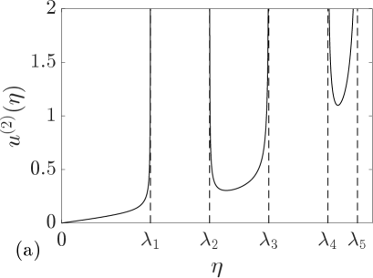
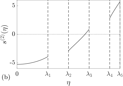
As an illustrative example we present in Fig. 1 the plots of the DOS and tracer velocity for the genus 2 soliton condensate.
We now consider slow modulations of non-equilibrium (non-uniform) soliton condensates by assuming , , . Equations (2.12), (3.10) then yield the kinetic equation for genus soliton condensate:
| (3.12) |
that is valid for . The velocity (3.11) then assumes the meaning of the tracer, or transport, velocity in a non-uniform genus soliton condensate.
Theorem 3.2.
The kinetic equation (3.12) for soliton condensate implies the evolution of the endpoints , according to the Whitham modulation equations
| (3.13) |
where and
| (3.14) |
Proof. (See [19]) Multiplying (3.12) by and passing to the limit we obtain equations (3.13), (3.14) for the evolution of the spectral -bands (i.e. the evolution of ). These are the KdV-Whitham modulation equations [4], [9] (see also Remark 3.2 below).
∎
Corollary 3.1.
The endpoints of the “special” band , , containing the point of zero tracer speed, , are moving in opposite directions, whereas all the endpoints on the same side from are moving in the same direction. See Fig. 1 (right) for
Remark 3.2.
Modulation equations (3.12), (3.13) were originally derived by Flaschka, Forest and McLaughlin [4] by averaging the KdV equation over the multiphase (finite-gap) family of solutions. These equations along with the condensate NDRs (3.5), also appear in the seminal work of Lax and Levermore [9] in the context of the semiclassical (zero-dispersion) limit of multi-soliton KdV ensembles (see Section 5 and, in particular, Equation (5.23) in [9]). A succinct exposition of the spectral Whitham theory for the KdV equation can be found in Dubrovin and Novikov [19]).
Remark 3.3.
The Whitham modulation equations (3.13), (3.14) are locally integrable for any via Tsarev’s generalized hodograph transform [20, 19]. Moreover, by allowing the genus to take different values in different regions of -plane, , global solutions of the KdV-Whitham system can be constructed for a broad class of initial data (see Section 4.2 for further details). Invoking the definitive property of a soliton condensate, the existence of the solution to an initial value problem for the Whitham system for all implies that this property will remain invariant under the -evolution, i.e. soliton condensate will remain a condensate during the evolution, however its genus can change.
The finite-genus Whitham modulation system (3.13), (3.14) can be viewed as an exact hydrodynamic reduction of the full kinetic equation (2.12), (2.11) under the ansatz (3.10), (3.11). Recalling the origin of the soliton gas kinetic equation as a singular, thermodynamic limit of the Whitham equations [3] the recovery of the finite-genus Whitham dynamics in the condensate limit might not look surprising. On the other hand, viewed from the general soliton gas perspective the condensate reduction notably shows that the highly nontrivial nonlinear modulation (hydro)dynamics emerges as a collective effect of the elementary two-soliton scattering events. This understanding is in line with ideas of generalised hydrodynamics, a powerful theoretical framework for the description of non-equilibrium macroscopic dynamics in many-body quantum and classical integrable systems [21]. The connection of the KdV soliton gas theory with generalised hydrodynamics has been recently established in [22]. Relevant to the above, it was shown in [23] that the semiclassical limit of the generalised hydrodynamics for the Lieb-Liniger model of Bose gases yields the Whitham modulation system for the defocusing NLS equation.
A different type of hydrodynamic reductions of the soliton gas kinetic equation defined by the multi-component delta-function ansatz for the DOS has been studied in [24] for and in [25, 26] for . One of the definitive properties of the multicomponent hydrodynamic reductions of this type is their linear degeneracy which, in particular, implies the absence of the wavebreaking and the occurrence of contact discontinuities in the solutions of Riemann problems [27]. In contrast, the condensate (Whitham) system (3.13), (3.14) obtained under the condition is known to be genuinely nonlinear, , [28] implying the inevitability of wavebreaking for general initial data, which is in stark contrast with linear degeneracy of the multicomponent “cold-gas” hydrodynamic reductions. Reconciling the genuine nonlinearity property of soliton condensates with linearly degenerate non-condensate multicomponent cold-gas dynamics is an interesting problem which will be considered in future publications.
Thus, we have shown that the spectral dynamics of soliton condensates are equivalent to those of finite gap potentials, which naturally suggests a close connection (or even equivalence) of these two objects at the level of realizations, i.e. the corresponding solutions of the KdV equation. This connection will be explored in the next section using a combination of analytical results and numerical simulations for genus 0 and genus 1 soliton condensates.
4 Genus 0 and genus 1 soliton condensates
Having developed the spectral description of KdV soliton condensates, we now look closer at the two simplest representatives: genus 0 and genus 1 condensates. In particular, we shall be interested in the characterization of the realizations of soliton condensates, i.e. the KdV solutions, denoted , corresponding to the condensate spectral DOS for . We do not attempt here to construct the soliton gas realizations explicitly via the thermodynamic limit of finite gap potentials (see Section 2), instead, we infer some of their key properties from the expressions (3.4) for the ensemble averages as integrals over the spectral DOS. We then conjecture the exact form of soliton condensate realizations and support our conjecture by detailed numerical simulations.
4.1 Equilibrium properties
4.1.1 Genus 0
For equations (3.10) for the DOS and the spectral flux density yield (cf. (2.16))
| (4.1) |
so that the tracer velocity (cf. (3.11))
| (4.2) |
Next, substituting (4.1) in (3.4) (where or equivalently, ), we obtain for the ensemble averages:
| (4.3) |
where . Thus the variance , which implies (see, e.g. [29]) that genus 0 soliton condensate is almost surely described by a constant solution of the KdV equation , i.e.
| (4.4) |
(note that constant solution is classified as a genus 0 KdV potential).
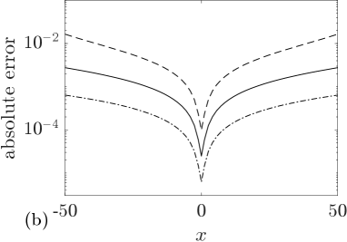
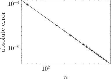
This result can be intuitively understood by identifying soliton condensate with the “densest possible” soliton gas for a given spectral support . The densest “packing” for genus 0 is achieved by distributing soliton parameters according to the spectral DOS (4.1) which results in the individual solitons “merging” into a uniform KdV field of amplitude . The numerical implementation of soliton condensate realizations, using -soliton KdV solution with large, shows that the condensate DOS (4.1) is only achievable within this framework if all solitons in the solution have the same phase of the respective norming constants. Invoking the interpretation of the phase of the norming constant as the soliton position in space [13, 30] one can say that in the condensate all solitons are placed at the same point, say (cf. Appendix A for a mathematical justification). Details of the numerical implementation of KdV soliton gas using -soliton solutions can be found in Appendix A. Fig. 2 displays the realization of genus 0 soliton condensate with modeled by -soliton solutions with and , along with the absolute errors ; in the following we refer to these -soliton solutions as “numerical realizations” of the soliton gas. One can see that the error at the center of the numerical domain, where the gas is nearly uniform, is very small: Fig. 3 displays the variation of this error with and shows that it decreases with .
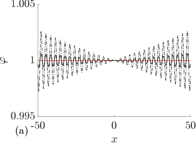
The numerical approximation used here is similar to the approximation of the soliton condensate of the focusing NLS equation via a -soliton solution presented in [50]. In the latter case the uniform wavefield limit as a central part of the so-called “box potential”, is also reached when the complex phases of the norming constants are chosen deterministically. The absolute error—the difference between the -soliton solution and the expected constant value of the wavefield—measured at the center of the numerical realization—follows a different scaling law and is proportional to .
4.1.2 Genus 1
We now consider the case of genus 1 soliton condensate. For
| (4.5) |
is purely imaginary on . According to Theorem 3.1
| (4.6) | ||||
| (4.7) |
where follows from the fact that . The normalization conditions (3.9) imply that
| (4.8) |
Using 3.131.3 and 3.132.2 from [31], we calculate
| (4.9) |
Calculation of is a bit more involved as it is based on the observation
| (4.10) |
Using (4.8), (4.10), we obtain after some algebra
| (4.11) |
Thus, the velocity of a tracer soliton with spectral parameter in the genus 1 soliton condensate, characterized by DOS (4.6), is given by
| (4.12) |
We note that a similar expression for the tracer velocity in a dense soliton gas was obtained in [32] in the context of the modified KdV (mKdV) equation.
For the integrals (3.4) for the mean and mean square of the soliton condensate wave field can be explicitly evaluated using (253.11) and (256.11) from [33] and 19.7.10 from [49]:
| (4.13) | |||
| (4.14) |
with and given by (4.9). It is not difficult to verify that, unlike in the case of genus 0 condensates, the variance does not vanish identically implying that all realizations of the genus 1 soliton condensate are almost surely non-constant.
A key observation is, that formulae (4.13), (4.14) coincide with the period averages and of the genus 1 KdV solution associated with the spectral Riemann surface of (4.5) (see e.g. [34, 35]):
| (4.15) |
where is an arbitrary initial phase.
The equivalence between the ensemble averages in genus 1 KdV soliton condensates and the period averages in single-phase KdV solutions, along with the established in Section 3 equivalence between the respective modulation dynamics, strongly suggest that realizations of the genus 1 soliton condensates are described by the periodic solutions (4.15) of the KdV equation. This motivates the following
Conjecture 4.1.
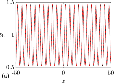
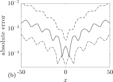
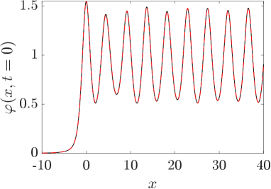
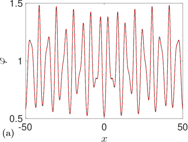
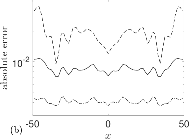
We support Conjecture 4.1 by a detailed comparison of a numerical realization of KdV soliton condensate (as -soliton solution with large) spectrally configured according to the DOS (4.6), and the periodic KdV solution (4.15), defined on the same spectral curve , with the appropriately chosen initial phase (see Appendix A for the details of the numerical implementation of soliton condensate). The comparison is presented in Fig. 4 and reveals a remarkable agreement, which further improves as increases.
Conjecture 4.1 can be naturally generalized to an arbitrary genus : for any realization of the KdV soliton condensate of genus corresponding to the density of states (3.10) and associated with the spectral Riemann surface of (3.8), one can find -component initial phase vector so that almost surely coincides with -phase KdV solution (2.5). To support this generalization we performed a comparison of a numerical realization of the genus 2 soliton condensate with the respective two-phase (two-gap) KdV solution, see Appendix B.
A rigorous mathematical proof of Conjecture 4.1 and its generalization for an arbitrary genus will be the subject of future work.
In conclusion we note that Conjecture 4.1 correlates with the results of [10] where a particular “deterministic soliton gas” solution of the KdV equation has been constructed by considering the -soliton solution with the discrete spectrum confined within two symmetric intervals—the analogs of s-bands of our work—and letting . This solution was shown in [10] to represent a primitive potential [36] whose long-time asymptotics is described at leading order by a modulated genus 1 KdV solution. A similar construction was realized for the mKdV equation in [32].
4.2 Modulation dynamics
The dynamics of DOS in non-equilibrium (weakly non-homogeneous) soliton condensates is determined by the evolution of the endpoints of the spectral bands of (the s-bands). As proven in Section 3, this evolution is governed by the Whitham modulation equations (3.13). Properties of the KdV-Whitam modulation systems are well studied: in particular, system (3.13) is strictly hyperbolic and genuinely nonlinear for any genus [28]. This implies inevitability of wavebreaking for a broad class of initial conditions. What is the meaning of the wavebreaking in the context of soliton condensates, and how is the solution of the kinetic equation continued beyond the wavebreaking time?
We first invoke the definitive property of a soliton condensate—the vanishing of the spectral scaling function, in the soliton gas NDRs (2.9). According to Remark 3.3, if for all , then for all , implying that soliton condensate necessarily remains a condensate during the evolution (at least of some class of initial data). The only qualitative modification that is permissible during the evolution is the change of the genus . The description of the evolution of a soliton condensate is then reduced to the determination of the spectral support , parametrizing the DOS via the band edges : (3.10).
In view of the above, the evolution of soliton condensates can be naturally put in the framework of the problem of hydrodynamic evolution of multivalued functions originally formulated by Dubrovin and Novikov [19]. Let be a smooth multivalued curve whose branches satisfy the Whitham modulation equations (3.13). Then, if wavebreaking occurs within one of the branches it results in a change of the genus so that in some space-time region that includes the wavebreaking point. The curves and are glued together at free boundaries . Details of the implementation of this procedure can be found in [19, 37, 38, 39]. The simplest case of the multivalued curve evolution arises when the initial data for is a piecewise-constant distribution (both for ’s and for ), with a discontinuity at — a Riemann problem. In this special case the wavebreaking occurs at (subject to appropriate sign of the initial jump) and smoothness of is not a prerequisite.
In this paper, we restrict ourselves to Riemann problems involving only genus 0 and genus 1 modulation solutions and show how the resulting spectral dynamics are interpreted in terms of soliton condensates. For that we will need explicit expressions for the Whitham characteristic velocities for and . These expressions are known very well (see e.g. [11, 34, 35]) but here we obtain them as transport velocities for the respective soliton condensates, using the expressions (4.2), and (4.12) respectively.
(i) . Consider a non-equilibrium (non-uniform) soliton condensate of genus 0, characterized by a space-time dependent DOS . To this end we set in (4.2), then the Whitham system (3.13), (3.14) assumes the form of the Hopf (inviscid Burgers) equation
| (4.16) |
Note that this is exactly the result obtained by Lax and Levermore [9] for the pre-breaking evolution of semi-classical soliton ensembles.
5 Riemann problem for soliton condensates
The classical Riemann problem consists of finding solution to a system of hyperbolic conservation laws subject to piecewise-constant initial conditions exhibiting discontinuity at . The distribution solution of such Riemann problem generally represents a combination of constant states, simple (rarefaction) waves and strong discontinuities (shocks or contact discontinuities) [41]. In dispersive hydrodynamics, classical shock waves are replaced by dispersive shock waves (DSWs) — nonlinear expanding wavetrains with a certain, well-defined structure [35]. Here we generalize the Riemann problem formulation to the soliton gas kinetic equation by considering (1.1) subject to discontinuous initial DOS:
| (5.1) |
where is the DOS (3.10) of genus condensate and .
As discussed in Section 4.2, soliton condensate necessarily retains its definitive property during the evolution, with the only qualitative modification permissible being the change of the genus . The evolution of the soliton condensate is then determined by the motion of the s-band edges according to the Whitham modulation equations (3.13) subject to discontinuous initial conditions following from (5.1):
| (5.2) |
Thus the Riemann problem for soliton gas kinetic equation is effectively reduced in the condensate limit to the Riemann problem (5.2) for the Whitham modulation equations (3.13). Depending on the sign of the jump the regularization of the discontinuity in can occur in two ways: (i) if then the regularization occurs via the generation of a rarefaction wave for without changing the genus of the condensate; (ii) if (which implies immediate wavebreaking for ) the regularization occurs via the generation of a higher genus condensate whose evolution is governed by the modulation equations.
Below we consider several particular cases of Riemann problems describing some prototypical features of the soliton condensate dynamics.
5.1
Consider the initial condition for the kinetic equation in the form of a discontinuous genus 0 condensate DOS,
| (5.3) |
where , and is defined in (4.1). The DOS distribution (5.3) implies the step initial conditions for the Whitham modulation system (3.13):
| (5.4) |
with . Additionally, since the wave field in a genus 0 soliton condensate is almost surely a constant, , we conclude that the DOS distribution (5.3) gives rise to the Riemann step data
| (5.5) |
for the KdV equation (2.1) itself.
The Riemann problem for the KdV equation was originally studied by Gurevich and Pitaevskii (GP) [11] in the context of the description of dispersive shock waves. The key idea of GP construction was to replace the dispersive Riemann problem (5.5) for the KdV equation by an appropriate boundary value problem for the hyperbolic KdV-Whitham system (4.17) which is then solved in the class of -self-similar solutions. Here we take advantage of the GP modulation solutions and their higher genus analogues to describe dynamics of soliton condensates. The choice of the genus of the Whitham system and, correspondingly, the genus of the associated soliton condensate, depends on whether or .
5.1.1 Rarefaction wave ()
The solution of the Riemann problem (1.1), (5.3) is given globally (for ) by the genus 0 DOS (4.1) modulated by the centered rarefaction wave solution of the Hopf equation (4.16) subject to the step initial condition (5.4):
| (5.6) |
where
| (5.7) |
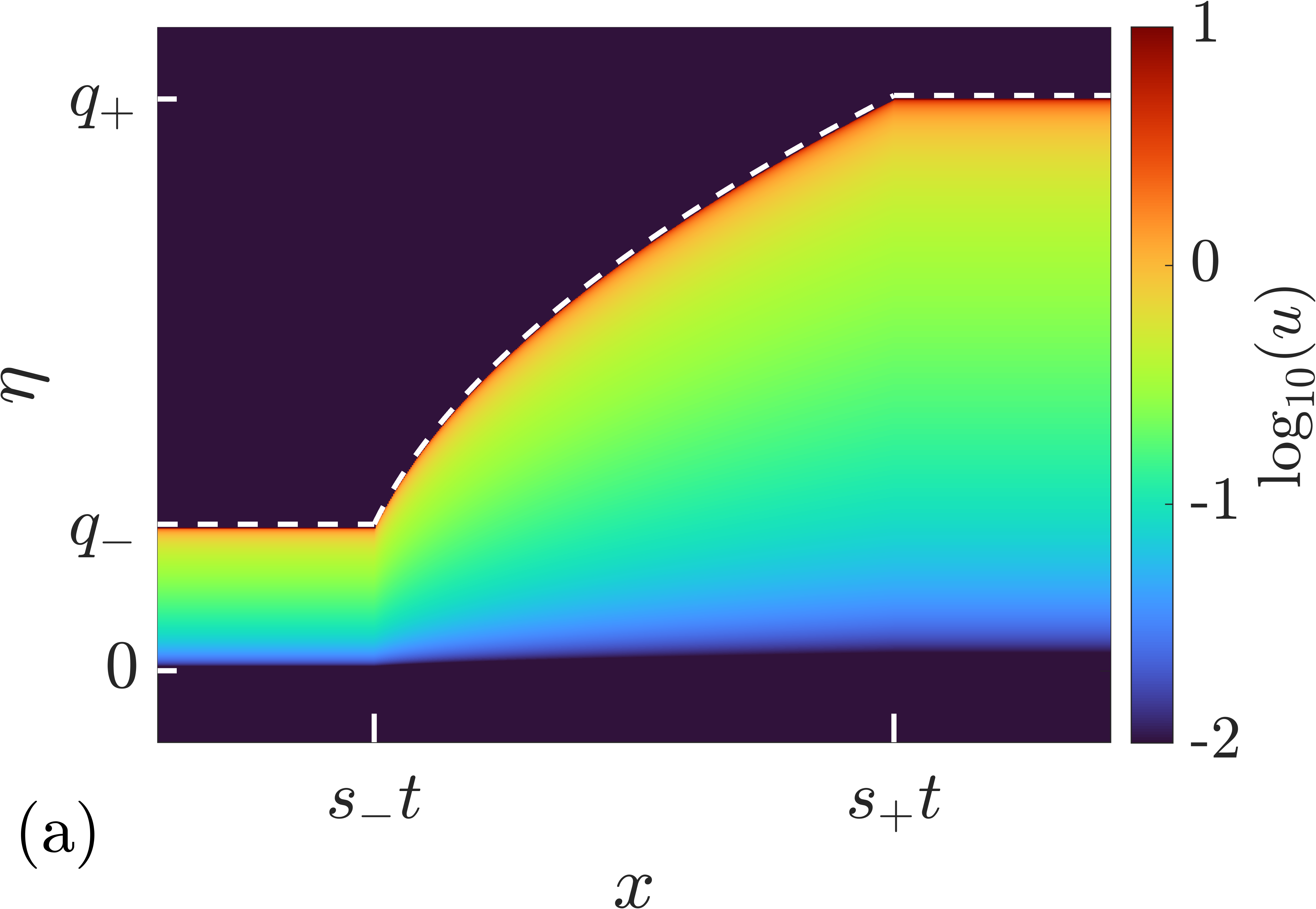
Note that the solution (5.6) is admissible since . Behavior of in the solution (5.6) is shown in Fig. 5a. The evolution of the soliton condensate’s DOS associated with the spectral rarefaction wave solution (5.6) is given by
| (5.8) |
5.1.2 Dispersive shock wave ()
The solution (5.6), (5.8) derived previously is not admissible for since in that case. In other words, the compressive discontinuous initial data (5.4) imply immediate wavebreaking and necessitate the introduction of the higher genus DOS connecting and . The requisite DOS is given by equation (4.6), which we reproduce here for convenience,
| (5.9) |
Here is given by (4.9) and , , are slowly modulated according to the Whitham equations (4.17), (4.18).
The solution of (4.18) is self-similar, , such that matches with at the left boundary , and with at the right boundary , with .
The requisite solution is the -wave of the Whitham system (4.17) (only is non-constant)
| (5.10) |
where
| (5.11) |
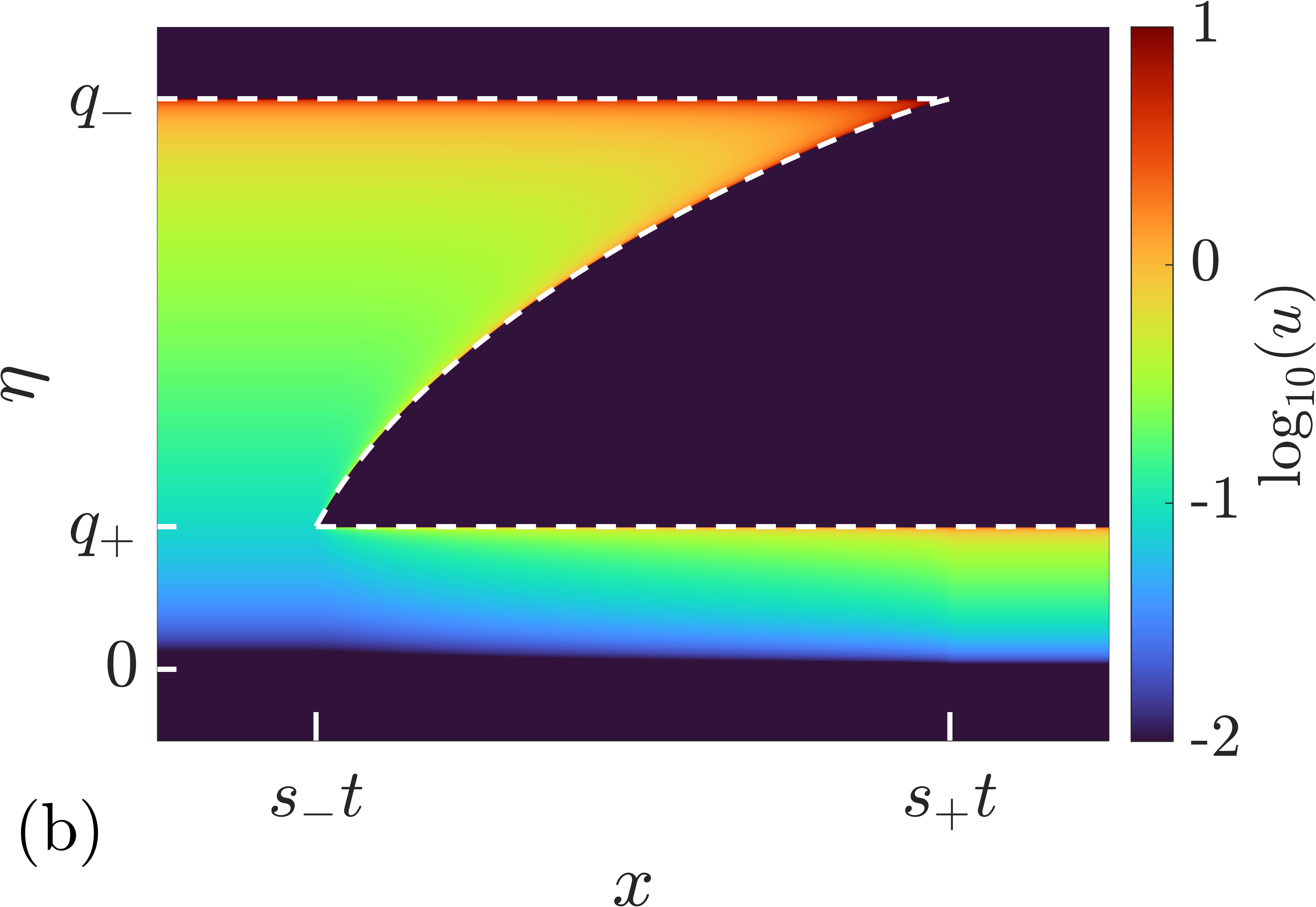
This is the famous GP solution describing the DSW modulations in the KdV step resolution problem [11]. Indeed, we have and, interpreting the GP solution (5.10) in terms of soliton condensates the limiting behaviors at the DSW edges is given by
| (5.12) |
5.2
Before considering the soliton condensate Riemann problem (1.1), (5.1) for the case we list the admissible solutions to the kinetic equation connecting a genus distribution to a genus distribution . One can easily verify for the next four solutions that
| (5.13) |
with .
We use the following convention to label the fundamental Riemann problem solutions: we call -wave, where is the index of the only varying Riemann invariant in the solution, while the remaining invariants are constant; indicates that i.e. the genus soliton condensate is initially at , and indicates that i.e. the genus soliton condensate is initially at .
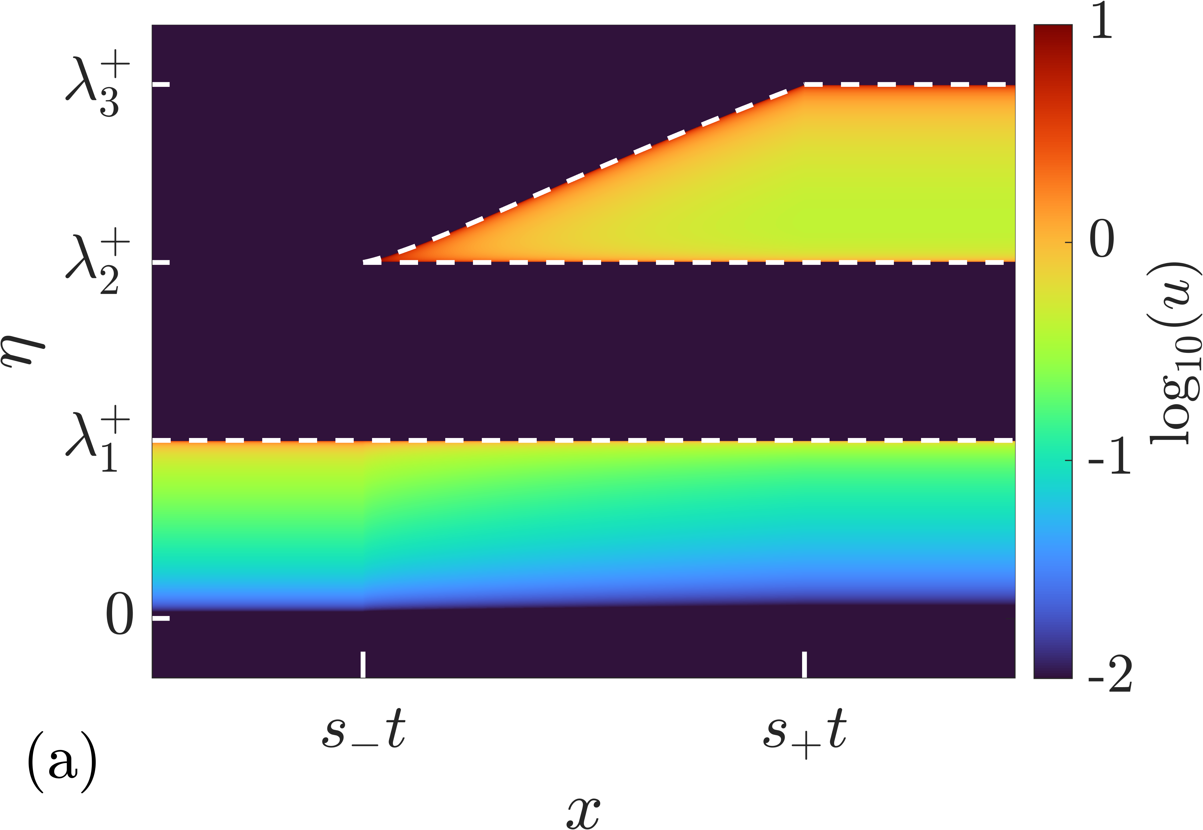
(i) -wave
Consider the initial condition for the soliton condensate DOS:
| (5.14) |
The resolution of the step (5.14) is described by
| (5.15) |
where is given by the -wave solution of the modulation equations (4.17):
| (5.16) |
The behavior of the Riemann invariants in the -wave is shown in Fig. 6a. The associated soliton condensate KdV solution along with the behavior of the mean are shown in Figs. 10 and 11.
(ii) -wave
Consider the initial condition:
| (5.17) |
The resolution of the step (5.17) is described by
| (5.18) |
where is given by the -wave solution of the modulation equations (4.17):
| (5.19) |
The behavior of the Riemann invariants in the -wave is shown in Fig. 6b.
(iii) -wave
Consider the initial condition:
| (5.20) |
The resolution of the step (5.20) is described by
| (5.21) |
where is given by the -wave solution of the modulation equations (4.17):
| (5.22) |
The behavior of the Riemann invariants in the -wave is shown in Fig. 6c.
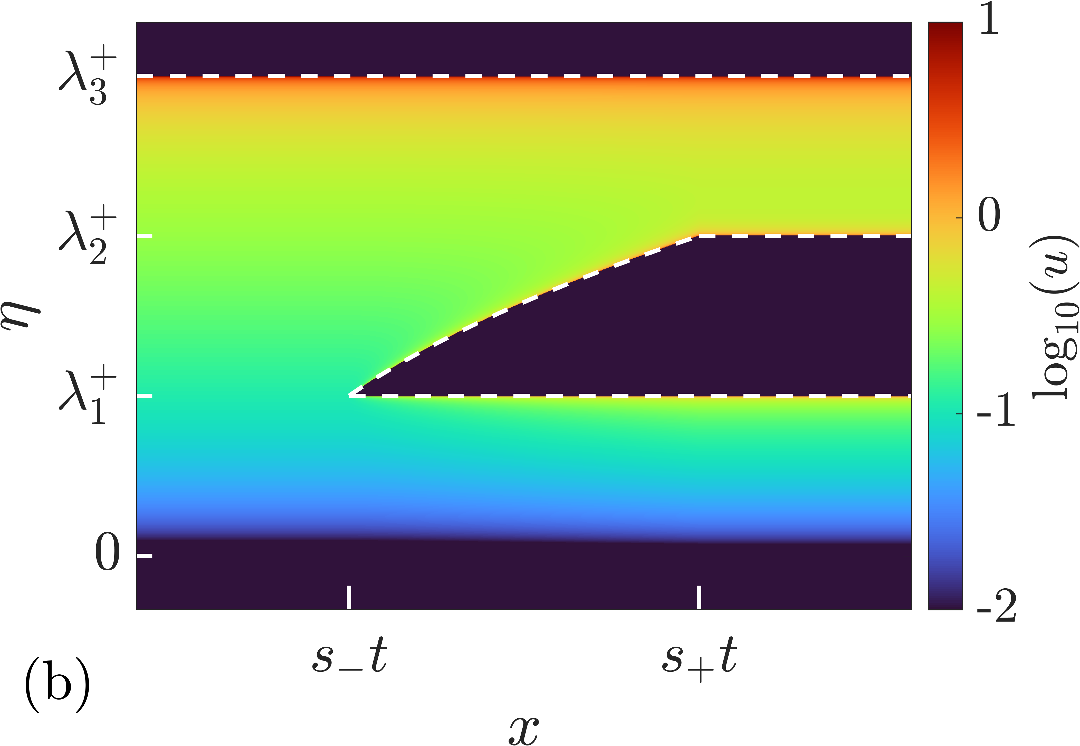
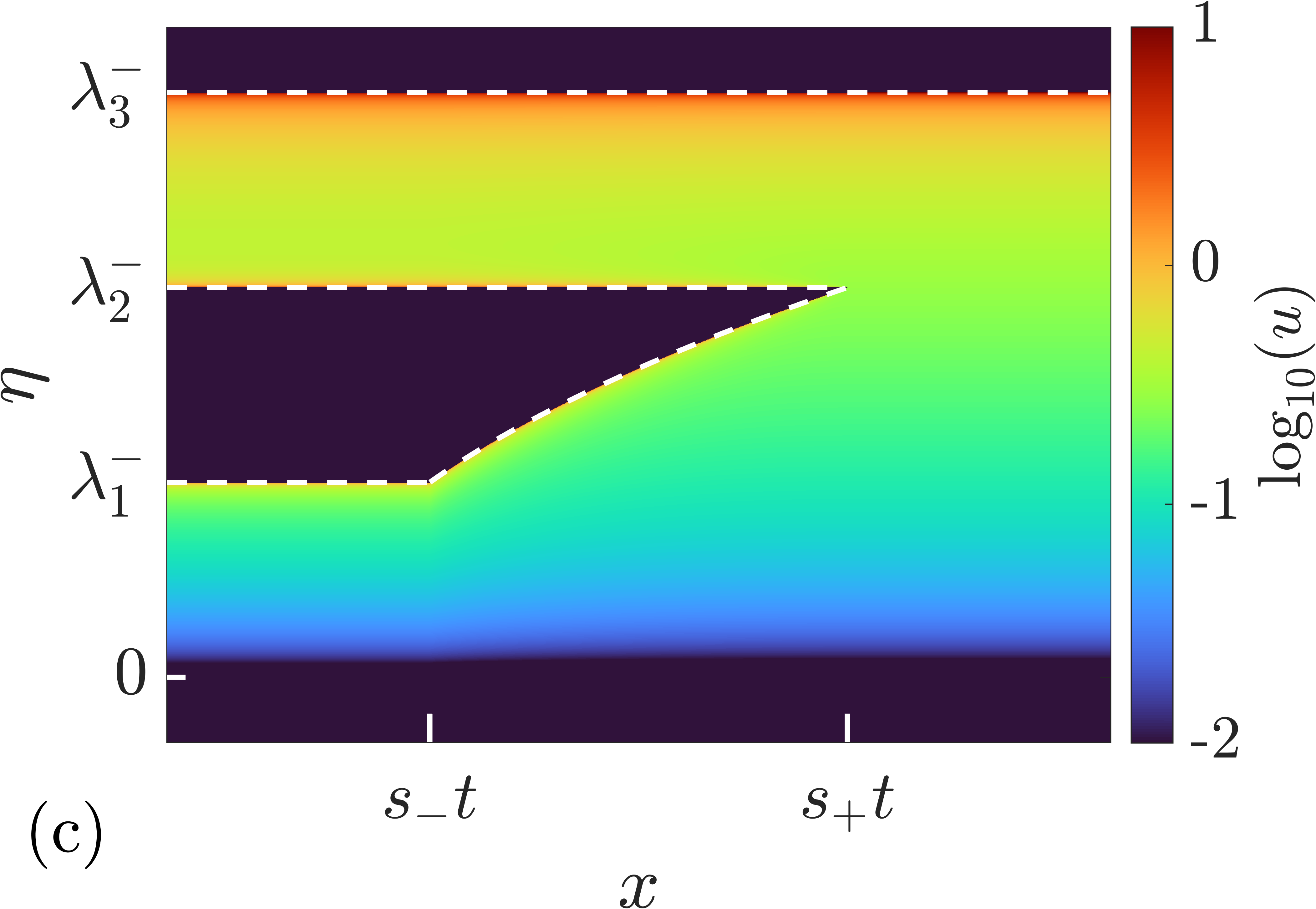
(iv) -wave
Consider the initial condition:
| (5.23) |
The resolution of the step (5.23) is described by
| (5.24) |
where is given by the -wave solution of the modulation equations (4.17):
| (5.25) |
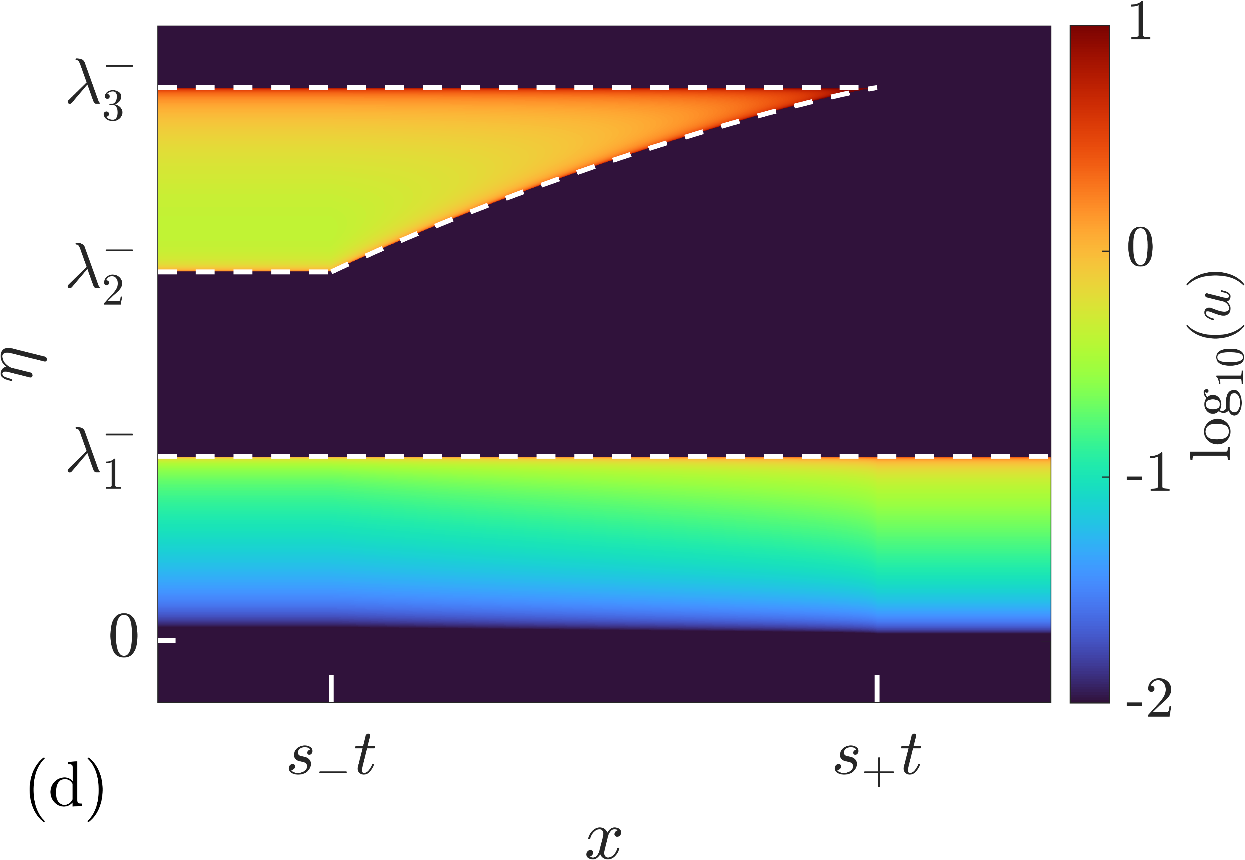
The behavior of the Riemann invariants in the -wave is shown in Fig. 6d. The associated soliton condensate KdV solution along with the behavior of the mean are shown in Figs. 12 and 13.
6 Riemann problem: numerical results
We consider Riemann problems with . Because of the inherent limitations of the numerical implementation of soliton gas detailed in Appendix A, we restrict the comparison to the cases or .
6.1 Rarefaction wave
In this first example, we choose
| (6.1) |
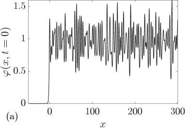
A numerical realization of the soliton condensate evolution corresponding to the steplike initial condition (6.1) is displayed in Fig. 7. The same figure displays the realization at . The realization corresponds to a -soliton solution with parameters distributed according to the initial DOS of (5.3), (6.1); details are given in Appendix A. As predicted in Sec. 4.1, the realization of the condensate corresponds to the vacuum at the left of , and a constant at the right of . As highlighted in Appendix A.1, the -soliton solution displays an overshoot at , regardless of the number of solitons , which is reminiscent of Gibbs’ phenomenon in the theory of Fourier series. This phenomenon has been originally observed in the numerical approximation of the soliton condensate of the focusing NLS equation by a -soliton solution in [50]; see for instance the similarities between Figs. 7a, 8b and Fig. 2a of [50]. Indeed, in both cases, the IST spectrum of the step distribution contains a non-solitonic radiative component (cf. [42]), which is not taken into account by the -soliton solution; the mismatch between the exact step and the -soliton solution manifests by the occurrence of the spurious oscillations observed near .
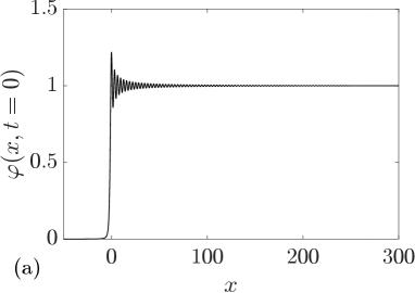
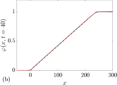
The solution of the Riemann problem with the initial condition (6.1) is given by where is the rarefaction wave (genus 0) solution (5.6). We have shown in Sec. 4.1 that the genus 0 soliton condensate is almost surely described by the constant solution . In the context of the evolution of the step (6.1) varies according to (5.6) so should be treated as a slowly varying (locally constant) condensate solution. In Fig. 7 we compare the numerical realization of the evolution of genus condensate with the analytical solution (5.6).
6.2 Dispersive shock wave
We now consider
| (6.2) |
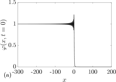
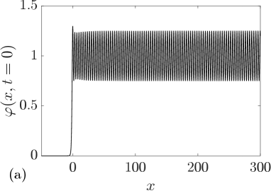
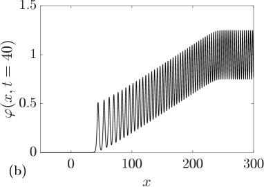
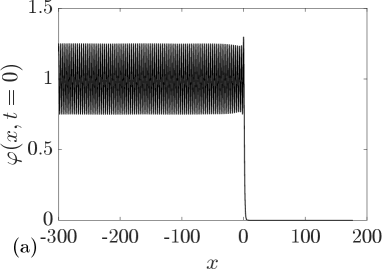
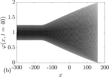
A numerical realization of the genus soliton condensate corresponding to the step-initial condition (6.2) is presented in Fig. 8 (a): it corresponds to the vacuum for , and a constant for . The realization at is shown in Fig. 8 (b) and it corresponds to a classical DSW solution for the KdV equation.
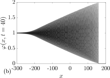
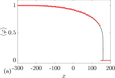
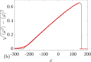
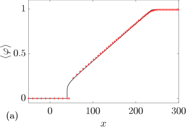
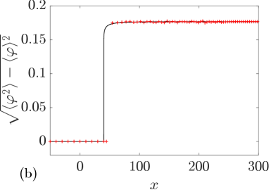
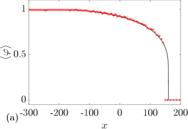
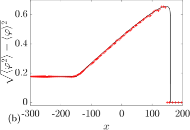
The solution of the condensate Riemann problem with the initial condition (5.3), (6.2) is given by the genus 1 DOS (5.9) modulated by the -wave solution (5.10) of the Whitham equations. In order to make a quantitative comparison of this analytical solution with the numerical evolution of the soliton gas displayed in Fig. 8, we compute numerically the mean and the variance , the latter being an amplitude type characteristic of the cnoidal wave. We have conjectured in Sec. 4.1 that any realization of the uniform genus condensate corresponds to a cnoidal wave modulo the initial phase . In that case, the ensemble average of the soliton condensate reduces to an average over the phase , or equivalently, over the period of the cnoidal wave, which can be performed on a single realization. We assume here that the result generalizes to non-uniform condensates so that the realization computed numerically and displayed in Fig. 8(b) can be consistently compared with a slowly modulated cnoidal wave solution. The averages and can be determined via a local phase average of one realization of the condensate. The local period averages are obtained via
| (6.3) |
where is the local wavelength extracted numerically.
The comparison between the analytically determined averages (4.13),(4.14),(5.10) and the averages (6.3) obtained numerically is presented in Fig. 11 and shows a very good agreement.
6.3 Generalized rarefaction wave
in the two previous examples. In the next examples, we choose . Let’s start with :
| (6.4) |
A numerical realization of the step-initial condition is displayed in Fig. 10. The same figure displays the realization at . The realization of the condensate corresponds to the “vacuum” for , and a cnoidal wave for . Note that the KdV equation does not admit heteroclinic traveling wave solutions, rendering difficult the numerical implementation of these “generalized” Riemann problems studied for instance in [43, 44]. Remarkably here, the solution depicted in Fig. 10 is an exact, -soliton solution of the KdV equation. As highlighted previously (see also Appendix A.1), the -soliton solution exhibits an overshoot at , regardless of the number of solitons .
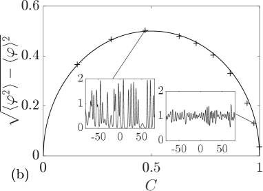
The solution of the Riemann problem for the kinetic equation with the initial condition (5.14), (6.4) is given by the -wave (5.15),(LABEL:eq:3-wave). The comparison between the analytical averages (4.13),(4.14),(LABEL:eq:3-wave) and the averages obtained numerically is shown in Fig. 11 and shows a very good agreement. The modulation depicted in Figs. 10b and 11a resembles the modulation of a cnoidal wave of an almost constant amplitude but with a varying mean. The variation of the mean is similar to the variation of the field in a classical rarefaction wave, so we call the corresponding structure shown in Fig. 10b a generalized rarefaction wave. The variance of the wavefield in the generalized rarefaction wave is shown in Fig. 11b.
6.4 Generalized dispersive shock wave
We now consider the “complementary” initial condition
| (6.5) |
An example of the numerical realization of the soliton gas step-initial condition and its evolution at are displayed in Fig. 12.
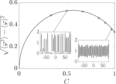
The solution of the Riemann problem with the initial condition (6.5) is given by the -wave (5.24), (5.25). The comparison between the analytically derived averages (4.13),(4.14),(5.25) and the averages obtained numerically is displayed in Fig. 13, and shows a very good agreement. The modulation observed in Figs. 12, 13 resembles the modulation of partial dispersive shock wave: the modulated cnoidal wave reaches the soliton limit for but terminates at for . The solution then continues as a non-modulated cnoidal wave for . This structure differs from the celebrated dispersive shock wave solution of the KdV equation involving the entire range [35]. We call the described structure connecting a constant state (a genus 0 condensate) at with a periodic solution (a genus 1 condensate) at a generalized DSW. We note that the soliton condensate structure shown in Fig. 12b exhibits strong similarity to the “deterministic KdV soliton gas” solution constructed in [10].
7 Diluted soliton condensates
7.1 Equilibrium properties
We now introduce the notion of a “diluted” soliton condensate by considering DOS , where is the condensate DOS of genus , and is the “dilution constant”.
E.g. the diluted soliton condensate of genus 0 is characterized by DOS
| (7.1) |
We recover the genus condensate DOS (4.1) by setting . As decreases, the “averaged spacing” between the solitons
| (7.2) |
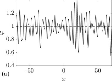
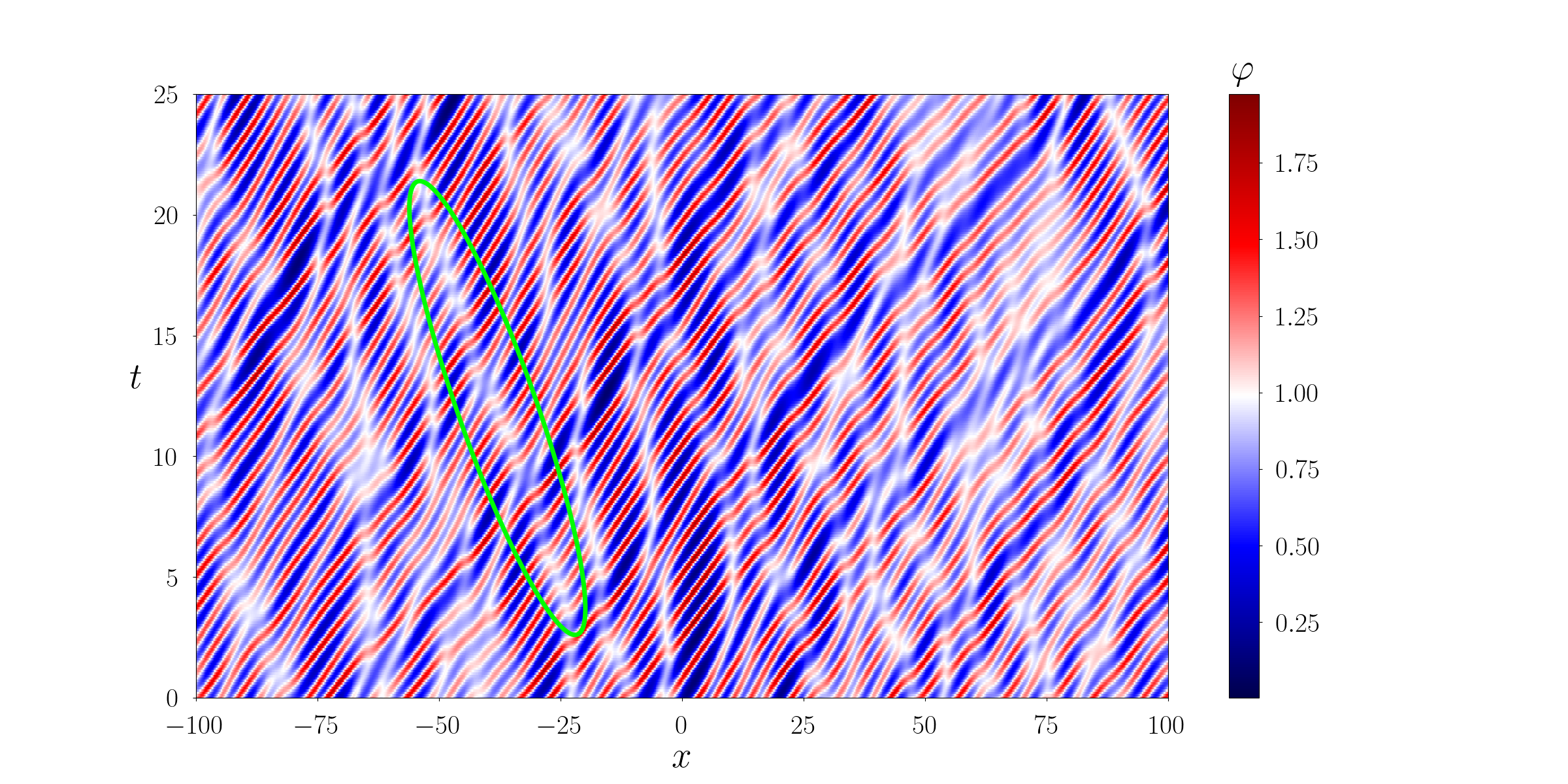
increases and the condensate gets “diluted”. Comparison between the most probable realization of the condensate () and a typical realization of a slightly dilute condensate () is given in Fig. 14. Remarkably, one can see that a slight increase of the average spacing between the solitons within the condensate results in the emergence of significant random oscillations of the KdV wave field.
As follows from (2.14) we have for the diluted genus 0 condensate so that the variance is given by:
| (7.3) |
The comparison between (7.3) and the variance obtained numerically by averaging over different diluted condensates is presented in Figure 14. Assuming ergodicity of a generic uniform soliton gas, the ensemble average in Fig. 14a (and Fig. 15) is computed here numerically with a spatial average of one, spatially broad, gas realization.
More generally, the diluted soliton condensate of genus is characterized by DOS
| (7.4) |
We have in the general case
| (7.5) |
where , are the ensemble averages obtained for the genuine condensate (), functions of only; for instance , are given by (4.13),(4.14). Since for and distinct ’s, the variance of diluted genus condensates
| (7.6) |
never vanishes if , as can be seen in the example shown in Fig. 15. Thus, in contrast with the genus 0 case, the transition from the genus 1 condensate () to diluted genus 1 condensate () does not see a drastic change in the oscillations’ amplitude. In particular, the oscillations seem to remain “almost” coherent – i.e. an average period can be identified – for the dilution factors close to 1 as depicted in the inset of Fig. 15.
Diluted condensates present a convenient framework to verify the prediction formulated in Remark 2.1 regarding the “backflow” effect (i.e. the existence of tracer KdV solitons moving in negative direction) in sufficiently dense soliton gases. A numerical simulation of the diluted genus condensate with where one can clearly see the soliton trajectory with a negative slope is presented in Fig. 16.
7.2 Riemann problem
We can now consider the soliton condensate Riemann problem for diluted condensates for which the initial DOS (5.1) is replaced by
| (7.7) |
where .
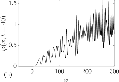
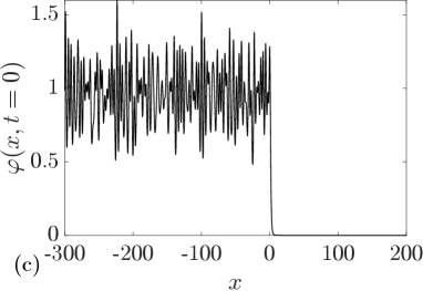
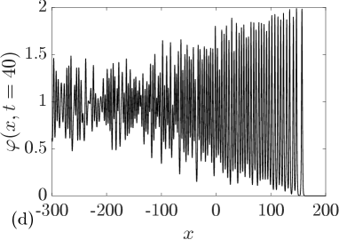
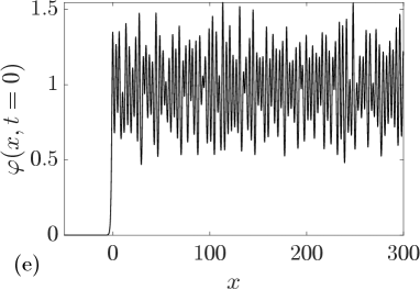
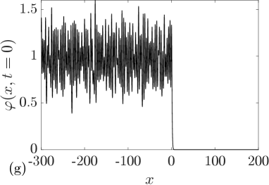
To be specific, we investigate numerically the evolution of the diluted condensate initial conditions (7.7) with and chosen from the examples presented in Sec. 6. Numerical realizations of the step-initial condition and their evolution in time are presented in Fig. 17. One can see that generally, realizations of the diluted soliton condensate do not exhibit a macroscopically coherent structure as observed in Sec. 6. However, in the case , the evolution of the diluted condensate realizations, despite the visible incoherence, still qualitatively resembles the evolution of the “genuine” condensates depicted in Figs. 10, 12. One can see that the recognizable patterns of the generalized rarefaction wave (see Fig. 17f) and the generalized DSW (see Fig. 17h) persist even if . Indeed, as shown in Sec. 7.1, the oscillations in a realization of the diluted genus 1 condensate appear almost coherent for a small dilution factor. The persistence of coherence can also be observed in the case when (Fig. 17d): a DSW develops if , and coherent, finite amplitude oscillations still develop for at the right edge of the structure where the amplitudes of oscillations are large. In connection with the above, it is important to note that, although the initial condition (7.7) is given by the discontinuous diluted condensate DOS, , the kinetic equation evolution does not imply that the DOS will remain to be of the same form for . In other words, unlike genuine condensates, the diluted condensates do not retain the spectral “diluted condensate” property during the evolution.

8 Conclusions and Outlook
We have considered a special kind of soliton gases for the KdV equation, termed soliton condensates, which are defined by the property of vanishing the spectral scaling function in the soliton gas nonlinear dispersion relations (2.9), (2.10). As a result, the density of states in a soliton condensate is uniquely determined by its spectral support . By considering to be a union of disjoint intervals, , and allowing the endpoints vary slowly in space-time we prove that the kinetic equation for soliton gas reduces in the condensate limit to the genus KdV-Whitham modulation for . The KdV-Whitham equations were originally derived via the wave averaging procedure in [40], [4] and via the semicalssical limit of the KdV equation in [9]. These equations have been extensively used for the description of dispersive shock waves [35], particularly in the context of dispersive Riemann problem originally introduced by Gurevich and Pitaevskii [11].
Along with the characterization of the large scale, modulation dynamics of soliton condensates, our work suggests that they represent “coherent” or “deterministic” soliton gases whose typical realizations are given by finite-gap potentials. We prove this conjecture for genus zero condensates and present a strong numerical evidence for .
By invoking the results from the modulation theory of dispersive shock waves we have constructed analytical solutions to several Riemann problems for the soliton gas kinetic equation subject to discontinuous condensate initial data. These solutions describe the evolution of generalized rarefaction and dispersive shock waves in soliton condensates. We performed numerical simulations of the Riemann problem for the KdV soliton condensates by constructing an exact -soliton solutions with large and the spectral parameters distributed according to the condensate densty of states. A comparison of the numerical simulations with analytical predictions from the solutions of the kinetic equation showed excellent agreement.
Finally, we considered the basic properties of “diluted” soliton condensates having a scaled condensate density of states and exhibiting rich incoherent behaviors.
There are several avenues for future work suggested by our results. One pertinent problem would be to consider near-condensate soliton gas dynamics by assuming the spectral scaling function to be “small” (, , ). Another area of major interest is the extension of the developed KdV soliton condensate theory to other integrable equations, particularly the focusing NLS equation, where a number of important theoretical and experimental results on the soliton gas dynamics have been obtained recently, see [55, 7, 60, 50]. And last but not least, one of the most intriguing open questions is the possibility of phase transitions in soliton gases, i.e. the formation of a soliton condensate from non-condensate initial data. The generalized hydrodynamics approach to the thermodynamics of soliton gases [22] provides a promising framework to explore this possibility. At the same time, this direction of research could require some departure from integrability and the development of the soliton gas theory for perturbed integrable equations.
Acknowledgments
The authors would like to thank the Isaac Newton Institute for Mathematical Sciences for support and hospitality during the programme “Dispersive hydrodynamics: mathematics, simulation and experiments, with applications in nonlinear waves” when the work on this paper was undertaken. This work was supported by EPSRC Grant Number EP/R014604/1. GE’s and GR’s work was also supported by EPSRC Grant Number EP/W032759/1 and AT’s work was supported by NSF Grant DMS 2009647. TC and GR thank Simons Foundation for partial support. All authors thank T. Bonnemain, S. Randoux and P. Suret for numerous useful discussions.
Appendix A Numerical implementation of soliton gas
A.1 Riemann problem
The realizations of the soliton gas are approximated numerically by the -soliton solution
| (A.1) |
where the ’s and ’s correspond respectively to the spectral parameters and the “spatial phases” of the solitons; by convention. The numerical implementation of (A.1) is described in Sec. A.3 below. The numerical solutions presented in this work are all generated with solitons, unless otherwise stated.
Since is finite, the -soliton solution reduces to a sum of separated solitons in the limit . By construction, we have in the limit
| (A.2) |
where are the spatial phases of the -th soliton at . We then take the spatial phase in (A.1) to be .
Consider a uniform soliton gas with the density of states . Let the spectral parameters be distributed on with density
| (A.3) |
where the normalization by the spatial density of solitons ensures that is normalized to . It was shown in [47] that the spatial density is obtained if the phases are uniformly distributed on the interval (denoted “-set” in [47]):
| (A.4) |
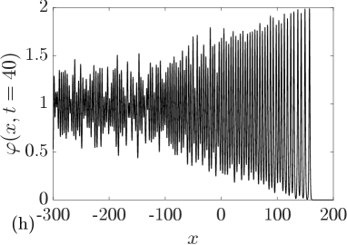
where is the spectral scaling function in the NDRs (2.9), (2.10); in [47] is given here by . The derivation of (A.4) has been revisited recently in the context of generalized hydrodynamics [22]: it was shown that corresponds to the density of spatial phases , or equivalently which are well defined asymptotically () where the solitons are “non-interacting” and their position are given by . In the rarefied gas limit the interaction term in the NDR (2.9) is small and therefore so that we obtain as expected. In the general case though the density of non-interacting phases is different from the “physical” density , as demonstrated with the soliton condensate examples below. In the thermodynamic limit , the soliton solution (A.1) represents a realization of the uniform soliton gas.
Since the number of solitons is finite, the -soliton solution has a finite spatial extent. By distributing the phases uniformly on the interval , the -soliton solution approximates a realization of the uniform soliton gas for where ; outside of this interval. This naturally generates the box-like initial condition for the kinetic equation
| (A.5) |
Note that can be seen as the genus condensate where the end point of the central s-band . This limits the type of initial condition that can be implemented for the Riemann problem and we choose in practice or . For convenience, we shift the -axis by to obtain one of the discontinuities at the position .
The evolution in time of the soliton gas realization is obtained by varying the parameter . Contrarily to a direct resolution of the KdV equation, via finite difference or spectral method, the time-evolution presented here is instantaneous and does not accumulate any numerical errors since the -soliton solution is an exact solution. For the Riemann problem, the maximal time is bounded by the finite extent of the -soliton solution: after a sufficently long time, the two hydrodynamic states originating from the discontinuities at and start interacting. Longer times can be reached by choosing a larger number of solitons .
We consider now the density of states of interest for this work:
| (A.6) |
where is density of states of the condensate defined in Sec. 3. (A.4) rewrites
| (A.7) |
Fig. 18 shows the comparison between the spatial density of solitons and the density of phases for the genus case where . The phases density diverges in the condensate limit , and ’s are all equal to the same phase (). This limit is in agreement with the results obtained in Sec. 4.1 for genus and genus condensates: each realisation of the condensate () is approximated with a coherent -soliton solution where .
Examples of numerical realizations of soliton condensates and diluted soliton condensates are given in Sections 4.1, 6, 7 and B. Figs. 2, 4 and 20 shows that numerical approximations of condensate via the -soliton solution are not exactly uniform; realizations become more uniform near the center of the interval as the number of soliton increases.
The realization at in Figs. 7, 8, 10 and 12 also displays the “border effects” observed at the discontinuities of the Riemann problem initial condition (located at ). These border effects, manifesting as overshoots of the realization, persist regardless of the number of solitons as shown by the comparison between the -soliton and -soliton solutions in Fig. 19. However, because of their finite size, the observed border effects seem to have no effect on the asymptotic dynamics of the condensate as demonstrated by the very good agreement between the theory and the numerical solution in Sec. 6.
A.2 Generation of spectral parameters
The spectral parameters of the -soliton solution are distributed with probability density , cf. (A.3). This can be achieved by choosing the solutions of the nonlinear equation
| (A.8) |
For genus 0 condensate whose DOS is given by (4.1), this equation reduces to
| (A.9) |
For genus 1 condensate with DOS (4.6), this equation reads
| (A.10) |
We have
| (A.11) |
which yields
| (A.12) |
where:
| (A.13) | |||
| (A.14) | |||
| (A.15) |
A.3 Algorithm for the -soliton solution
The algorithm generating the exact -soliton (A.1), originally developed in [45], relies on the Darboux transformation. This scheme is subject to roundoff errors during summation of exponentially small and large values for a large number of solitons . We improve it following [46], with the implementation of high precision arithmetic routine to overcome the numerical accuracy problems and generate solutions with a number of solitons .
In order to simplify the algorithm, it is suggested to consider simultaneously the KdV equation (2.1) and its equivalent form
| (A.16) |
obtained from (2.1) by the reflection . The Darboux transformation presented here relates the Jost solution associated with the -soliton solution of one equation, to the -soliton solution of the other equation.
Considering the direct scattering problem for the Lax pair in the matrix form
| (A.17) |
with corresponding to (2.1) and to (A.16), the Jost solutions are defined recursively by the Darboux transformations and such that:
| (A.18) |
| (A.19) |
and are independent of and have the form:
| (A.20) |
with the real constants depending on the spatial phases
| (A.21) |
The Jost solutions for the initial seed solution are given by
| (A.22) |
and one can show that at each recursion step
| (A.23) |
where is the -soliton solution of (2.1) for even and solution of (A.16) for odd. Recently, a more efficient and accurate algorithm has been proposed in [51] to generate the -soliton KdV solution employing a -fold Crum transform.
Appendix B Genus condensate
In Fig. 20 a realization of the genus 2 soliton condensate is compared with the two-phase KdV solution associated with the same spectral surface and equipped with an appropriately chosen initial phase vector. The two-phase solution has been computed numerically using the so-called trace formula [13]:
| (B.1) |
where the auxiliary spectra satisfy Dubrovin’s ordinary differential equations:
| (B.2) |
with and
| (B.3) |
Each oscillates in the corresponding s-gap so that the sign of changes every time changes direction of motion at the gap end point. We observe that, to compute the KdV finite-gap solution corresponding to a given realization soliton condensate, all the initial phases must be placed at the edges of the corresponding s-gaps while the choice of the gap’s edge (right/left) is determined by the number of discrete eigenvalues (odd/even) that are located within the s-band in the numerical construction of the condensate.
References
- [1] V. E. Zakharov, “Turbulence in integrable systems,” Studies in Applied Mathematics, vol. 122, pp. 219–234, 2009.
- [2] V. Zakharov, “Kinetic equation for solitons,” Journal of Experimental and Theoretical Physics, vol. 33, pp. 538–541, 1971.
- [3] G. El, “The thermodynamic limit of the Whitham equations,” Physics Letters A, vol. 311, pp. 374–383, 2003.
- [4] H. Flaschka, M. G. Forest, and D. W. McLaughlin, “Multiphase averaging and the inverse spectral solution of the Korteweg-de Vries equation,” Comm. Pure Appl. Math., vol. 33, pp. 739–784, 1980.
- [5] G. A. El and A. M. Kamchatnov, “Kinetic equation for a dense soliton gas,” Physical Review Letters, vol. 95, p. 204101, Nov 2005.
- [6] T. Congy, G. El, and G. Roberti, “Soliton gas in bidirectional dispersive hydrodynamics,” Physical Review E, vol. 103, p. 042201, 2021.
- [7] G. El and A. Tovbis, “Spectral theory of soliton and breather gases for the focusing nonlinear Schrödinger equation,” Physical Review E, vol. 101, p. 052207, 2020.
- [8] A. Kuijlaars and A. Tovbis, “On minimal energy solutions to certain classes of integral equations related to soliton gases for integrable systems,” Nonlinearity 34 no. 10 7227 (2021)
- [9] P. D. Lax and C. D. Levermore, “The small dispersion limit of the Korteweg-de Vries equation: 2,” Comm. Pure Appl. Math., vol. 36, no. 5, pp. 571–593, 1983.
- [10] M. Girotti, T. Grava, and K. D. T.-R. McLaughlin, “Rigorous asymptotics of a KdV soliton gas,” Comm. Math. Phys., vol. 384, pp. 733–784, 2021.
- [11] A. V. Gurevich, L. P. Pitaevskii, Nonstationary structure of a collisionless shock wave, Sov. Phys. JETP 38 (2) (1974) 291–297, translation from Russian of A. V. Gurevich and L. P. Pitaevskii, Zh. Eksp. Teor. Fiz. 65, 590-604 (August 1973).
- [12] G.A. El, “Soliton gas in integrable dispersive hydrodynamics,” J. Stat. Mech.: Theor. Exp. 114001, 2021.
- [13] S. P. Novikov, S. Manakov, L. P. Pitaevskii, and V. Zakharov, Theory of Solitons: The Inverse Scattering Method. Monographs in Contemporary Mathematics, Springer, 1984.
- [14] S. Venakides, “The continuum limit of theta functions,” Communications on Pure and Applied Mathematics, vol. 42, no. 6, pp. 711–728, 1989.
- [15] A. Tovbis and F. Wang, “ Recent developments in spectral theory of the focusing NLS soliton and breather gases: the thermodynamic limit of average densities, fluxes and certain meromorphic differentials; periodic gases,” arXiv:2203.03566.
- [16] E. Pelinovsky and E. Shurgalina. KDV soliton gas: interactions and turbulence. In Advances in Dynamics, Patterns, Cognition, 295-306, Springer, Cham., 2017
- [17] F. Tricomi, “On The Finite Hilbert Transformation,” Q J Math, vol. 2, no. 1, pp. 199–211, 1951.
- [18] S. Okada and D. Elliot, “The finite Hilbert transform in ,” Mathematische Nachrichten, vol. 153, no. 1, pp. 43–56, 1991.
- [19] B. A. Dubrovin and S. P. Novikov, “Hydrodynamics of weakly deformed soliton lattices. Differential geometry and Hamiltonian theory,” Russian Mathematical Surveys, vol. 44, no. 6, pp. 35–124, 1989.
- [20] S. P. Tsarëv, “The geometry of Hamiltonian systems of hydrodynamic type. the generalized hodograph method,” Mathematics of the USSR-Izvestiya, vol. 37, pp. 397–419, Apr 1991.
- [21] B. Doyon. Lecture notes on Generalised Hydrodynamics. In SciPost Physics Lecture Notes, page 18, 2020.
- [22] T. Bonnemain, B. Doyon and G. A. El , Generalized hydrodynamics of the KdV soliton gas, Journ. Phys. A: Math. Theor. 2022 (accepted), arXiv:2203.08551
- [23] E. Bettelheim. The Whitham approach to the limit of the Lieb–Liniger model and generalized hydrodynamics. Journal of Physics A: Mathematical and General, 53:205204, 2020.
- [24] G. A. El, A. M. Kamchatnov, M. V. Pavlov, and S. A. Zykov, “Kinetic Equation for a Soliton Gas and Its Hydrodynamic Reductions,” Journal of Nonlinear Science, vol. 21, pp. 151–191, 2011.
- [25] M. V. Pavlov, V. B. Taranov, and G. A. El, “Generalized hydrodynamic reductions of the kinetic equation for a soliton gas,” Theoretical and Mathematical Physics, vol. 171, pp. 675–682, 2012.
- [26] E.V. Ferapontov and M.V. Pavlov, Kinetic Equation for Soliton Gas: Integrable Reductions, J. Nonlin. Sci., 32, 26, 2022
- [27] F. Carbone, D. Dutykh, and G. A. El, “Macroscopic dynamics of incoherent soliton ensembles: Soliton gas kinetics and direct numerical modelling,” EPL (Europhysics Letters), vol. 113, p. 30003, 2016.
- [28] C.D. Levermore, The hyperbolic nature of the zero dispersion KdV limit, Comm. Part. Diff. Eq., 13, 495-514, 1988.
- [29] V. K. Rohatgi and A.K.Md. Ehsanes Saleh, An introduction to probability and statistics, vol. 1. John Wiley & Sons, 2015.
- [30] P. Drazin and R. Johnson, Solitons: an Introduction, 2nd ed. Cambridge University Press, 1989.
- [31] I. S. Gradshteyn, I. M. Ryzhik and R. H. Romer, Tables of integrals, series, and products, 1988.
- [32] M. Girotti, T. Grava, R. Jenkins, K. McLaughlin, A. Minakov, Soliton v. the gas: Fredholm determinants, analysis, and the rapid oscillations behind the kinetic equation, arXiv:2205.0260, 2022.
- [33] P. F. Byrd and M. D. Friedman, Handbook of elliptic integrals for engineers and physicists, Springer-Verlag, 1954.
- [34] A. M. Kamchatnov, Nonlinear periodic waves and their modulations: an introductory course. World Scientific, 2000.
- [35] G. El and M. Hoefer, “Dispersive shock waves and modulation theory,” Physica D: Nonlinear Phenomena, vol. 333, pp. 11–65, Oct 2016.
- [36] S. Dyachenko, D. Zakharov, and V. Zakharov, “Primitive potentials and bounded solutions of the KdV equation,” Physica D: Nonlinear Phenomena, vol. 333, pp. 148–156, 2016.
- [37] B. Dubrovin, Functionals of the Peierls-Frölich type and variational principle for Whitham equations, Amer. Math. Soc. Transl. 179 (1997) 35-44
- [38] G. A. El, A. L. Krylov, S. Venakides, Unified approach to KdV modulations, Comm. Pure Appl. Math. 54 (2001) 1243–1270.
- [39] T. Grava, F.-R. Tian, The generation, propagation, and extinction of multiphases in the KdV zero-dispersion limit, Comm. Pur. Appl. Math. 55 (12) (2002) 1569–1639.
- [40] G. B. Whitham, “Non-linear dispersive waves,” Proc. Roy. Soc. Ser. A, vol. 283, pp. 238–261, 1965.
- [41] P. D. Lax, Hyperbolic systems of conservation laws and the mathematical theory of shock waves. SIAM, 1973.
- [42] M. J. Ablowitz, Nonlinear dispersive waves: asymptotic analysis and solitons. Cambridge University Press, 2011.
- [43] P. Sprenger, and M. A. Hoefer, “Discontinuous shock solutions of the Whitham modulation equations as zero dispersion limits of traveling waves.” Nonlinearity 33 no. 10 3268 (2020).
- [44] S. Gavrilyuk, B. Nkonga, K. M. Shyue and L. Truskinovsky, “Stationary shock-like transition fronts in dispersive systems”, Nonlinearity, 33 no. 10 5477 (2020).
- [45] Nian-Ning Huang. “Darboux transformations for the Korteweg-de-Vries equation”. Journal of Physics A: Mathematical and General, 25(2):469, 1992.
- [46] A.A. Gelash and D.S. Agafontsev. Strongly interacting soliton gas and formation of rogue waves. Phys. Rev. E, 98(4):042210, 2018.
- [47] A. V. Gurevich, N. G. Mazur, K. P. Zybin, “Statistical limit in a completely integrable system with deterministic initial conditions,” Journal of Experimental and Theoretical Physics, 90, pp. 695–713, 2000.
- [48] P. J. Prins and S. Wahls, “An accurate floating point algorithm for the Crum transform of the KdV equation”, Commun Nonlinear Sci Numer Simul, 102, 105782 (2021)
- [49] F. W. J. Olver, A. B. Olde Daalhuis, D. W. Lozier, B. I. Schneider, R. F. Boisvert, C. W. Clark, B. R. Miller, B. V. Saunders, H. S. Cohl, and M. A. McClain, eds., NIST Digital Library of Mathematical Functions. http://dlmf.nist.gov/, Release 1.1.6 of 2022-06-30.
- [50] A. Gelash, D. Agafontsev, P. Suret, and S. Randoux, “Solitonic model of the condensate”, Phys. Rev. E, 104(4):044213, 2021.
- [51] P. J. Prins and S. Wahls, “An accurate floating point algorithm for the Crum transform of the KdV equation”, Commun Nonlinear Sci Numer Simul, 102, 105782 (2021)
- [52] B. Doyon, “Lecture notes on Generalised Hydrodynamics”, SciPost Physics Lecture Notes, 018 (2020)
- [53] T. Bonnemain, G. El, and B. Doyon, “Generalized hydrodynamics of the KdV soliton gas”, J. Phys. A: Math. Theor., 55, 374004, 2022.
- [54] E. Bettelheim, ‘The Whitham approach to the limit of the Lieb–Liniger model and generalized hydrodynamics”, J. Phys. A: Math. Theor., 53, 205204, 2020.
- [55] A. Gelash, D. Agafontsev, V. Zakharov, G. El, S. Randoux, and P. Suret, “Bound State Soliton Gas Dynamics Underlying the Spontaneous Modulational Instability”, Phys. Rev. Lett., 123, 234102, 2019.
- [56] D. Agafontsev and V. Zakharov, “Integrable turbulence and formation of rogue waves”, Nonlinearity, 28, 2791–2821, 2015.
- [57] D. Agafontsev, S. Randoux, and P. Suret, “Extreme rogue wave generation from narrowband partially coherent waves”, Phys. Rev. E, 103(3):032209, 2021.
- [58] E. D. Belokolos, A. I. Bobenko, V. Z. Enolski, A. R. Its, and V. B. Matveev, Algebro-geometric approach to nonlinear integrable equations. New York: Springer, 1994.
- [59] V. B. Matveev, “30 years of finite-gap integration theory,” Philosophical Transactions of the Royal Society A: Mathematical, Physical and Engineering Sciences, vol. 366, no. 1867, pp. 837–875, 2008.
- [60] G. Roberti, G. El, A. Tovbis, F. Copie, P. Suret, and S. Randoux, “Numerical spectral synthesis of breather gas for the focusing nonlinear Schrodinger equation”, Phys. Rev. E, 103(4):042205, 2021.