Dissipative Magnetohydrodynamics for Non-Resistive Relativistic Plasmas:
An implicit second-order flux-conservative formulation with stiff relaxation
Abstract
Based on a 14-moment closure for non-resistive (general-) relativistic viscous plasmas, we describe a new numerical scheme that is able to handle all first-order dissipative effects (heat conduction, bulk and shear viscosities), as well the anisotropies induced by the presence of magnetic fields. The latter is parameterized in terms of a thermal gyrofrequency or, equivalently, a thermal Larmor radius and allows to correctly capture the thermal Hall effect. By solving an extended Israel-Stewart-like system for the dissipative quantities that enforces algebraic constraints via stiff-relaxation, we are able to cast all first-order dissipative terms in flux-divergence form. This allows us to apply traditional high-resolution shock capturing methods to the equations, making the system suitable for the numerical study of highly turbulent flows. We present several numerical tests to assess the robustness of our numerical scheme in flat spacetime. The 14-moment closure can seamlessly interpolate between the highly collisional limit found in neutron star mergers, and the highly anisotropic limit of relativistic Braginskii magnetohydrodynamics appropriate for weakly collisional plasmas in black-hole accretion problems. We believe that this new formulation and numerical scheme will be useful for a broad class of relativistic magnetized flows.
I Introduction
Relativistic fluid dynamics is widely used as an effective description of long wavelength, long time phenomena in a variety of many-body systems such as the quark-gluon plasma Romatschke and Romatschke (2019), the early universe Weinberg (2008), and the hot and ultradense matter formed in neutron star mergers Baiotti and Rezzolla (2017). In the context of heavy-ion collisions, experiments at the Relativistic Heavy Ion Collider and the Large Hadron Collider have provided overwhelming evidence that the quark-gluon plasma formed in highly energetic nuclear collisions behaves as a strongly-interacting relativistic fluid over distance scales not much larger than the size of a nucleus Heinz and Snellings (2013). Through the last decade (see Romatschke and Romatschke (2019) for a review), detailed comparisons between numerical hydrodynamic simulations and experimental data have shown that the matter formed in such collisions is not a perfect fluid, i.e., viscous effects are needed to describe experimental data. In fact, the quantitative extraction of the transport coefficients (such as shear and bulk viscosities) of the quark-gluon plasma from heavy-ion collision data Bernhard et al. (2019); Nijs et al. (2021); Everett et al. (2021a, b) provides key guidance toward understanding the novel out-of-equilibrium properties that emerge in deconfined quark-gluon matter at extreme temperatures and moderate baryon densities.
Hydrodynamic simulations of the quark-gluon plasma in heavy-ion collisions solve second-order relativistic viscous hydrodynamic equations of motion Israel and Stewart (1979), which may be obtained from entropy considerations, relativistic kinetic theory, or from a resummation of the gradient series Baier et al. (2008). Current formulations in use Baier et al. (2008); Denicol et al. (2012) share the same spirit of Israel-Stewart theory Israel and Stewart (1979) in which dissipative corrections to the energy-momentum tensor and the conserved currents behave as new degrees of freedom that obey additional (relaxation-type) equations of motion, which must be solved together with the conservation laws to determine the evolution of the fluid. Alternative formulations, such as anisotropic hydrodynamics Martinez and Strickland (2010); Florkowski and Ryblewski (2011); Bazow et al. (2014); Alqahtani et al. (2018, 2017), have also been used in heavy-ion simulations.
In the linearized regime around equilibrium, it is known that there are conditions involving the equation of state and the transport coefficients which, once fulfilled, guarantee stability and causality of second-order theories Hiscock and Lindblom (1983); Olson (1990). In the nonlinear regime probed in heavy-ion collisions, however, the backreaction from the dissipative corrections becomes important and more stringent conditions to ensure causality have been derived Bemfica et al. (2019a, 2021). See Chiu and Shen (2021); Plumberg et al. (2021) for discussions on the relevance of such nonlinear causality conditions in the description of the evolution of the quark-gluon plasma.
Numerical implementations of viscous, Israel-Stewart-like equations of motion can be found both in Eulerian Romatschke and Romatschke (2007); Schenke et al. (2012); Bozek (2012); Del Zanna et al. (2013); Karpenko et al. (2014); Shen et al. (2016); Habich et al. (2015); Romatschke (2015); Bazow et al. (2018); Okamoto and Nonaka (2017) and also in Lagrangian algorithms Noronha-Hostler et al. (2013, 2014, 2016). In the former, numerical methods originally written to solve flux conservative problems are adapted Jeon and Heinz (2015) to determine the evolution of the system, even though the second-order viscous formulations Denicol et al. (2012); Baier et al. (2008) employ equations of motion that are, in general, not in flux conservative form. In the latter, a Lagrangian method based on Smoothed Particle Hydrodynamics Monaghan (1992), extended to the relativistic regime Aguiar et al. (2001), is used in heavy-ion simulations Noronha-Hostler et al. (2013, 2014, 2016).
In the context of neutron star mergers, effective dissipation is crucial to model the correct equilibrium of accretion disks Shakura and Sunyaev (1973) and capture potentially out-of-(weak)-equilibrium effects that could affect the gravitational wave emission Alford et al. (2018); Most et al. (2021) or late time evolution of the remnant Radice (2017); Fujibayashi et al. (2018); Shibata et al. (2017); Fujibayashi et al. (2020). Moreover, turbulent dynamo processes in the merger Price and Rosswog (2006); Kiuchi et al. (2015); Aguilera-Miret et al. (2020); Skoutnev et al. (2021) critically depend on the presence of a resistive and a viscous scale. In the case of Rayleigh-Taylor instabilities potentially present at the surface of the merging neutron stars, the amplification and growth scale might depend critically on the shear viscosity Skoutnev et al. (2021).
Several attempts have been made to incorporate viscosity into astrophysical fluid dynamics simulations of relativistic systems. In the context of black hole accretion and neutron star merger remnants, some have considered simple (and acausal Hiscock and Lindblom (1985)) Navier-Stokes approaches, e.g. Ref. Duez et al. (2004); Fragile et al. (2018), whereas more recently Israel-Stewart-like formulations have been considered in Ref. Shibata et al. (2017); Chabanov et al. (2021). Apart from second-order formulations, recent progress in causal and hyperbolic first-order theories Bemfica et al. (2018); Kovtun (2019); Bemfica et al. (2019b); Hoult and Kovtun (2020); Bemfica et al. (2020) has also enabled the first simulations of such theories in the context of conformal relativistic fluids Pandya and Pretorius (2021). Another conceptually very different approach with symmetric hyperbolic structure originating from the study of continuum mechanism was presented by Refs. Peshkov et al. (2019); Romenski et al. (2020). In the context of mimicking effective shear viscous dissipation associated with small-scale magnetic turbulence, large-eddy closures have been proposed Radice (2017, 2020), although additional effort is required to ensure covariance of such a closure Duez et al. (2020). In the same spirit, an effective Israel-Stewart shear viscous formulation was proposed in Shibata et al. (2017) and successfully applied to long-term studies of post-merger remnants Fujibayashi et al. (2018).
In this work we take a different approach in that we consider dissipative evolution equations derived from a moment expansion of the relativistic Boltzmann equation Denicol et al. (2012). Going beyond all works above, we include all first-order dissipative effects, such as heat conduction, bulk and shear viscosity, and also include the anisotropies induced by magnetic fields in the equations of motion of the dissipative quantities in a fully covariant way. The only effect omitted here is resistivity, which we will consider in a forthcoming study. To this end, we incorporate the gyrofrequency as a free parameter, which allows us to control the degree of anisotropy of heat conduction and shear stresses relative to the direction of the (comoving) magnetic field. Critically, Ref. Denicol et al. (2018) has shown that in a systematic expansion in inverse Reynolds and Knudsen numbers, the associated magnetic field coupling considered in this work is the only possible term that appears at first and second order in a gradient expansion, if resistive effects of the plasma are neglected (see Denicol et al. (2019) for the resistive case). For extreme magnetic field strengths relative to the plasma energy, which are not considered here, additional terms might have to be added at second-order, though Panda et al. (2021).
Additionally, one issue affecting all previous numerical (Eulerian)
implementations of Israel-Stewart formulations is the appearance of source
terms with time derivatives. While the presence of strong shocks and fluid
gradients in turbulent astrophysical scenarios calls for high-resolution
shock capturing (HRSC) schemes, these derivatives are not commonly treated
in this way, see e.g. Del Zanna et al. (2013).
This can easily lead to
numerical instabilities in the flow in more complex simulations, if the dissipative terms develop
gradients themselves, which is associated with regions of numerically under-resolved
physical viscosity. In this work, we address this point in full, by
carefully designing an HRSC scheme, where all first-order dissipation terms
are treated in flux-divergence form Toro (2013). This is facilitated by the use of
stiff relaxation terms that are treated with implicit time integration
schemes Pareschi and Russo (2005). The use of such stiff relaxation terms
is inspired by the implementation of the force-free electrodynamics
limit in numerical relativity simulations
Alic et al. (2012); Palenzuela (2013); Most and Philippov (2020). Overall, this makes our
scheme suitable for applications in heavy-ion collisions and astrophysical
fluid dynamics alike.
This paper is structured as follows. In Sec. II we describe the equations of motion we employ and in Sec. III we provide a detailed derivation of how to recast them in flux-divergence form. In Sec. IV, we describe the numerical method used to solve these equations, and in particular how we handle stiff source terms. In Sec. V we demonstrate the ability of this scheme to successfully model relevant test problems, and provide a discussion of the results in Sec. VI. Throughout this paper, we adopt geometrical units where and a mostly plus signature for the Lorentzian spacetime metric .
II Non-Resistive Relativistic Dissipative Magnetohydrodynamics
A relativistic ideal fluid can be described via its rest-mass (“baryon”) density , energy density , and four-velocity (normalized such that ). The equilibrium pressure is defined in terms of the other thermodynamic variables such that, for instance, . This defines the equation of state, with which one may compute the temperature using standard thermodynamic relations. The equilibrium hydrodynamics system can be described by means of an energy-momentum tensor
| (1) |
where
| (2) |
is the rank-2 projector orthogonal to the flow velocity, i.e. . Conservation of baryon number is defined in terms of the rest-mass current and baryon number conservation
| (3) |
In this work we will also consider the effects of a (co-moving) magnetic field tightly coupled to the fluid, i.e. in the limit of infinite electric conductivity Denicol et al. (2018). We note that so that, in the local rest frame of the fluid where , the magnetic field 4-vector only has nonzero spatial components.
The electromagnetic field is described by the electromagnetic field strength tensor and its dual
| (4) | |||
| (5) |
We stress again that these expressions only hold in the limit infinite electric conductivity, in which the comoving electric field vanishes. For later convenience, we have also introduced above the shorthand notation . The evolution of the magnetic field is then governed by the Maxwell equation , which may be written as
| (6) |
It is useful to introduce the projector
| (7) |
which is orthogonal to and . Using this projector, it can be shown that
| (8) |
and
| (9) |
The electromagnetic fields give rise to an energy-momentum tensor given by Duez et al. (2005)
| (10) |
In total, the generalized energy-momentum tensor for non-resistive ideal magnetohydrodynamics can be written as
| (11) |
The equations of motion of ideal relativistic magnetohydroynamics stem from the conservation of energy and momentum
| (12) |
coupled to Eq. (6).
II.1 Second-order hydrodynamic equations
In the following we summarize a formalism for describing out-of-equilibrium dynamics allowing for viscous corrections to the system. These can be encoded by the viscous stress tensor , which is added to the fluid’s energy-momentum tensor. In this work, we use the so-called Eckart hydrodynamic frame Eckart (1940) in which the rest-mass current remains , all viscous/dissipative effects appear only in the expression for the energy-momentum tensor, and there are no out-of-equilibrium corrections to the energy density.
Considering the number of degrees of freedom, we can see that and have a total of 14 (since is symmetric), but in equilibrium only five of them are actually independent (e.g. ). Accounting for out-of-equilibrium dynamics of the system then amounts to prescribing evolution equations for the remaining 9 degrees of freedom. These can be parameterized in terms of the bulk scalar pressure , the symmetric anisotropic pressure tensor , and the heat flux , which obey a distinct set of constraints on the dissipative momenta and stresses, i.e.
| (13) | ||||
| (14) | ||||
| (15) |
Therefore, once these constraints are fulfilled, the set indeed only has 9 independent degrees of freedom. As we show in this paper, the way these constraints are imposed heavily influences the numerical methods required to study this system. Overall, we can group these contributions into the viscous stress tensor
| (16) |
which is then added to the hydrodynamics equations
| (17) |
The combined stress-energy tensor, including the dissipative contributions, is covariantly conserved
| (18) |
whereas remains unchanged with dynamics given by (3). We point out that we choose the Eckart frame in this work solely for numerical convenience in the context of astrophysical applications. Clearly, other definitions of the hydrodynamic fields, i.e. other hydrodynamic frames Israel and Stewart (1979), could have been used. For instance, one could have removed the heat flux and introduced a diffusive correction to the baryon current. Alternatively, one may employ other frames in which both terms are present. For a deeper discussion about hydrodynamic frames, and how a judicious choice of hydrodynamic variables can be useful to formulate causal, stable and strongly-hyperbolic theories of viscous relativistic fluids at first-order in derivatives, see Bemfica et al. (2018); Kovtun (2019); Bemfica et al. (2019b); Hoult and Kovtun (2020); Bemfica et al. (2020). Second-order Israel-Stewart-like theories in general hydrodynamic frames have also been investigated in Tsumura and Kunihiro (2010), and more recently in Noronha et al. (2021); Rocha and Denicol (2021).
Having parameterized the viscous degrees of freedom, we need to prescribe a set of causal evolution equations for them. In this work, we use equations of motion obtained from a truncation of suitably defined moments of the relativistic Boltzmann-Vlasov equation for a gas of charged particles (without dipole moment or spin) dynamically coupled to a magnetic field. This approach to obtain the second-order hydrodynamic equations employs a systematic expansion of the Boltzmann equation in powers of the Knudsen and inverse Reynolds numbers111The Knudsen numbers measure the ratio between microscopic length scales and the macroscopic scales associated with gradients of the conserved quantities. In the approach of Denicol et al. (2012), one denotes quantities such as as inverse Reynolds numbers, given that they can be seen as relativistic generalizations of the ratio between viscous and inertial forces., and this method was originally applied in Denicol et al. (2012) in the investigation of neutral kinetic systems. The equations of motion, and the transport coefficients obtained within this formulation, are widely used in current heavy-ion collision simulations of the quark-gluon plasma (usually done in the absence of eletromagnetic fields). This formalism was extended to include non-resistive, comoving magnetic field effects using the Boltzmann-Vlasov equation in Denicol et al. (2018). The magnetohydrodynamical equations of motion were obtained in the so-called 14-moment approximation Israel and Stewart (1979) and they essentially provide a generalization of Israel-Stewart fluid dynamics to the case of non-vanishing magnetic fields. The full resistive case (which includes effects from comoving electric and magnetic fields) was worked out later in this approach in Ref. Denicol et al. (2019).
In our work, the dissipative variables obey the following advection-type relaxation equations222We note that the original derivation of the non-resistive equations of motion in Denicol et al. (2018) used the Landau frame Landau and Lifshitz (1987). The Eckart frame version of these equations can be found by taking the non-resistive limit of the equations derived in Denicol et al. (2019).
| (19) | |||
| (20) | |||
| (21) |
where we have introduced the symmetric trace-free projector
| (22) |
Above, is the shear viscosity, is the bulk viscosity, is the thermal conductivity, is the bulk relaxation time, is the relaxation time for heat flux, while is the shear viscosity relaxation time. Besides those coefficients, the equations of motion also contain the additional second-order transport coefficients and the new coefficients that determine the coupling between the dissipative quantities and the electromagnetic field tensor, and . Expressions for all of these coefficients, including and , in terms of the temperature and chemical potential for an ultrarelativistic gas can be found in Denicol et al. (2012, 2019, 2018). In this work, we treat the ratios ,, , , , , , as free parameters defined in terms of thermodynamic quantities ( and ). It is important to remark that in the formulation of Ref. Denicol et al. (2018) the form of the equations of motion remains very close to that found in standard Israel-Stewart theory, with additional terms that couple the fluid variables directly to the magnetic field. Also, we note that in this first work we have not included all the possible second-order terms that appear in Denicol et al. (2012, 2018, 2019). A systematic investigation of their effects will be given in a forthcoming study.
We note that any second-order theory with relaxation equations for the dissipative currents given by (19), (20), and (21) has an asymptotic relativistic Navier-Stokes regime. This can be seen by performing a systematic expansion in gradients, together with the conservation laws Baier et al. (2008). In the absence of magnetic fields, to first order in gradients the system reduces to
| (23) | ||||
| (24) | ||||
| (25) |
which is the standard relativistic generalization of Navier-Stokes theory Eckart (1940). It is important to understand that this limit can never be reached exactly, since it reduces the character of the hydrodynamic evolution equations from hyperbolic to parabolic, rendering the system acausal Pichon (1965). Also, we note that the standard constraints that stem from a linearized analysis of causality and stability, derived in the absence of a magnetic field in Hiscock and Lindblom (1983), automatically hold for the system of equations we use. For a linearized study of stability and causality in the presence of a nonzero magnetic field, see Biswas et al. (2020).
III Flux-conservative formulation
In the following, we will reformulate the equations for the bulk pressure (19), heat flux (20), and shear-stress tensor (21) in a flux-conservative form Toro (2013); Rezzolla and Zanotti (2013) that is suitable for numerical simulations. In particular, we will suitably extend the system in a way that allows us to recast all first-order gradient terms into flux-divergence form, i.e. , for a suitable flux function . To this end, to better illustrate our approach, we consider all viscous effects separately.
III.1 Bulk pressure
We start out by considering the Israel-Stewart-like equation (19) for the bulk pressure . After a simple algebraic manipulation it can be shown that Eq. (19) is equivalent to
| (26) |
Here we have introduced the shorthand . We will provide a detailed treatment of arbitrary viscous relaxation terms in Sec. III.5. We note that depending on the application this equation can be further simplified.
In the simplest case of , or if is advected, i.e. and , we find
| (27) |
which, remarkably, is free of derivatives on the right-hand side (RHS).
III.1.1 Limit of vanishing relaxation time
We now consider a particular limit of these equations, showing that in the limit of vanishing relaxation time the system does not always approach to a perfect fluid solution. Indeed, we can see from Eq. (27) that for a choice of transport coefficient , with , the limit corresponds to the introduction of a newly conserved quantity, i.e.
| (28) |
where conservation is to be understood to hold approximately up to second-order corrections. Physically, this limit is reached when bulk viscous damping happens on viscous scales much larger than the dynamical scale . We can further see that in this limit, satisfies a continuity equations, akin to the baryon density . In the absence of effective viscous damping, this implies that provides an effective correction to the equation of state, which now depends on the bulk viscous scalar , and in turn on the velocity via the continuity equation. This is similar to the use of microphysical equations of state that depend on compositional information, given by an advected scalar, such as the electron fraction Oertel et al. (2017).
III.2 Heat conduction
Next we turn to the equation for heat conduction. It can trivially be shown that
| (29) |
where we have used that . The specific form of this equation further allows us to add terms proportional to , since these get projected out by the global projection. Along those lines, it will help us to simplify the equations if we add such a terms in the following way
| (30) |
We can now understand the meaning of the projector in Eq. (29) as follows.
Contracting Eq. (29) with , we see that the
sole purpose of the projector is to enforce Eq. (13), such that is orthogonal to .
In practice, the presence of such a projector will lead to a variety of
gradient terms, which explicitly impose the
constraint (29). Such terms are typically numerically
difficult to evaluate and will not only increase the error budget of any
numerical solution, but they will also numerically lead to only an
approximate enforcement of Eq. (13).
A better approach, which is commonly used in relativistic force-free
electrodynamics Alic et al. (2012); Palenzuela (2013), is to instead include the constraint (29)
via stiff relaxation Alic et al. (2012).
Introducing a new relaxation time , we can
equivalently write
| (31) |
The effect of this term can best be considered in the Navier-Stokes limit (in the absence of magnetic fields), where
| (32) |
Hence, the constraint (13) will indeed be imposed when . Although Eq. (31) is more desirable from a numerical point of view than the original Israel-Stewart equation (20), we will need implicit numerical schemes in order to properly compute this term. This will be explained in detail in Sec. IV. Applying the same reordering that leads to a flux-conservative form (26) for the bulk scalar we obtain the final form
| (33) |
For a class of theories, where or advected , and , we find the simple flux-conservative stiff relaxation equation
| (34) |
Nonetheless, our numerical scheme is able to solve systems with arbitrary heat conductivities, see Sec. III.5.
III.2.1 Comparison with non-relativistic heat conduction
It is interesting to consider a simple limiting case in order to highlight the nature of heat conduction within this formulation. Restricting ourselves to flat spacetime, zero magnetic field, and assuming a vanishing 3-velocity (i.e. ), it can be shown (neglecting dissipative sources other than heat condution) that the equations reduce to
| (35) | |||
| (36) |
For simplicity, adopting the ideal gas law , where is the Boltzmann constant , the baryon mass and the adiabatic coefficient, we find
| (37) |
In this simple example, we have used that for vanishing fluid velocity. In the Navier-Stokes limit where , we find that this expression reduces to the standard heat equation. However, because this limit will not be reached and instead we find that the temperature evolution obeys
| (38) |
This is a damped wave equation for the temperature with wave speed
| (39) |
where causality places a strict bound on . This is nothing but the Telegrapher’s equation, which has already been extensively studied in the context of hyperbolic heat conduction (see, e.g. Romatschke (2010a)).
III.3 Shear-viscous stresses
We finally consider the evolution of the shear stress tensor , with the aim of recasting it into flux-conservative form. Starting from Eq. (21), we write
| (40) |
where . Similar to the observations made for Eq. (29), we find that the introduction of the trace-free projector was done to ensure the validity of the constraints (14) and (15). In the same spirit of deriving Eq. (31), we can replace the projector by the introduction of a stiff relaxation current. More specifically, we write
| (41) |
where we have introduced the relaxations times . Reordering the terms in the same way as for Eqs. (26) and (33), we find
| (42) |
We further note that all terms terms proportional to are already accounted for in the constraint damping term and will get removed in the limit. Remarkably, and differently from the heat conduction and bulk viscosity, this leads to the removal of the term from the equations. Hence, no approximation or other special treatment need to be applied to handle non-constant shear viscosity. The final form of the evolution equation then reads
| (43) |
As a final remark we stress the ambiguity in adding or removing constraint terms related to Eq. (14) and (15). While in the continuum limit Eq. (15) will perfectly hold, the discrete version of these equations might behave differently whether or not additional terms proportional to would be added. One particular example would be the removal of the trace from the shear tensor in Eq. (43). This would lead to a replacement of the principal part of Eq. (43) with
| (44) |
Whether or not such modifications will impact the stability of the system will require a more in-depth analysis, which will be provided in forthcoming work.
III.4 Interpretation of the magnetic field coupling
In the following, we would like to associate a meaning with the magnetic field coupling terms, and . To facilitate this, we will draw on an analogy with the Ohm’s law for a single fluid ideal magnetohydrodynamics in the Newtonian regime. To this end, we consider a simple Ohm’s law from Hall magnetohydrodynamics Sturrock and Andrew (1994),
| (45) |
where is the electron gyrofrequency, the electron charge, the electron mass and the electric current.
By fixing the gyration velocity , we can also express this via the inverse Larmor radius .
Taking the Newtonian limit of Eq. (20), i.e. , and going to the rest-frame of the fluid , we obtain
| (46) |
Since we only consider non-resistive plamas, we can see that the heat conduction current replaces the electric current compared to Eq. (45). In fact, if we were to consider resistive plasmas Denicol et al. (2019), we would obtain exactly the same expression with on the RHS, where is the comoving electric field, and the associated conductivity.
Although Eq. (45) describes an electric and Eq. (46) a heat current, it can be shown that the two are related in a dissipative relativistic fluid description. Indeed, the total heat flux of the theory is given by Denicol et al. (2019)
| (47) |
where is the baryon mass and is the particle diffusion current, which directly enters
the electric current in Maxwell’s equations Denicol et al. (2019).
In defining the dissipative system in Eq. (16), we have
made a frame choice, to neglect the particle diffusion current,
and treat the heat flux vector directly. We could have
additionally chosen to operate in the Landau frame, and instead
reexpressed the system in terms of the diffusion current ,
being more similar to Eq. (45).
Overall, this comparison allows us to identify the coupling scale with a thermal gyrofrequency
| (48) |
We further find it natural to identify the time scale of collisions with the relaxation time , as those should be proportional to each other. Physically this implies that the thermal conductivity (in the Navier-Stokes limit) will split into a part parallel and perpendicular , to the magnetic field, where the latter term is the equivalent of the electric Hall conductivity Denicol et al. (2018). In particular, this would lead to an anisotropic modification of the Navier-Stokes limit as follows
| (49) |
Crucially, in our current prescription these anisotropy effects are controlled by a single parameter , which can be freely specified. For a more detailed discussion of this effect, see Ref. Denicol et al. (2018).
III.4.1 Braginskii-limit
Having discussed that the equations presented here are naturally able to capture the effect of (Hall) anisotropies in the heat conduction, we now turn to the strong coupling limit. It will turn out that this limit has a very important interpretation in the limit of weakly collisional plasmas.
Indeed, in the strong coupling limit , we find that the shear stress and heat flux must satisfy
| (50) | |||
| (51) |
Since and are also subject to the constraints (13)-(15), we find that this imposes the following form on the dissipative fluxes and stresses,
| (52) | |||
| (53) |
where and are Lorentz scalars, which in the Navier-Stokes limit approach
| (54) | |||
| (55) |
From a physical point of view, can be identified with the mean-free-path of the system Denicol et al. (2018) so that, as expected, in the limit of weak collisionality a Braginskii-like limit is recovered Braginskii (1965) for our system of equations.
A similar formulation of relativistic viscous magnetohydrodynamics using Israel-Stewart-like equations has been proposed for weakly collisional plasmas in Ref. (Chandra et al., 2015). This formulation was modelled after non-relativistic Braginskii theory (Braginskii, 1965), where the shear stress aligns with the comoving magnetic fields. We stress that differently from the formulation of Chandra et al. (2015) where the anisotropy of the viscous stresses and heat flux has been imposed from the outset, in the framework considered here the anisotropy emerges naturally as the gyrofrequency diverges in the limit of weak collisionality plasmas. As such, the (truncated first-order) equations of Denicol et al. (2018) in this limit can be considered as a generalization of Braginskii magnetohydrodynamics for non-resistive relativistic plasmas for finite thermal gyrofrequencies.
III.5 Advection terms
Although we have so far managed to eliminate most gradient terms from the RHS of the equations of motion, a set of advection and compression terms still remain. We will now, likewise, reformulate them as a set of implicit rate equations in the comoving frame.
We note that because of baryon number conservation, an arbitrary advected scalar satisfies
| (56) |
If we want to enforce that follows a certain behavior, , we may implicitly define an autonomous source term such that
| (57) |
This gives rise to a relaxation current
| (58) |
where is a stiff relaxation time scale. In order to enforce the condition (57) we may add this current to the advected part,
| (59) |
In other words, in the local comoving frame of the fluid, this equation is prescribing a rate equation to enforce the damping of towards on a (subgrid) time scale . If we can evaluate the stiff current numerically, it can be used to replace advective derivatives of the form
| (60) |
In the same way, we can also treat gradient terms by noting that
| (61) |
where is the Kronecker symbol. Introducing the current , we can write in non-covariant form:
| (62) |
where is the Christoffel symbol associated with and
| (63) |
Here is a stiff relaxation timescale.
Applied to our source terms this results in the following set of stiff advection equations
| (64) | |||
| (65) | |||
| (66) | |||
| (67) | |||
| (68) |
The source terms of those equations are fixed according to
| (69) | |||
| (70) | |||
| (71) | |||
| (72) | |||
| (73) |
where we have introduced new relaxation time scales .
III.6 Summary
In conclusion, our equations of motion for flux-conservative dissipative magnetohydrodynamics read
| (74) | |||
| (75) | |||
| (76) | |||
| (77) | |||
| (78) | |||
| (79) | |||
| (80) | |||
| (81) | |||
| (82) | |||
| (83) |
Before we proceed, a few comments are in order. All second-order gradient terms on the RHS of all equations are treated implicitly via the relaxation equations associated with (57). Although such a treatment seems approximate, compared to the flux-divergence operator on the left-hand side (LHS), it is important to point out that we are primarily interested in near-equilibrium behavior where , , and are small. As such, these specific second-order terms constitute only a minor correction and could even be omitted. This is also consistent with neglecting all other second-order transport terms in these equations, which should otherwise be present Denicol et al. (2012). On the other hand, since first-order gradient terms are important for the evolution, they require more sophisticated numerical methods, as outlined in Sec. IV . Second, we point out that in deriving these equations we have made use of our freedom to remove all terms proportional to on the RHS. Due to the projected nature of the Israel-Stewart limit, these terms would get removed when projecting the equations into the fluid frame (in the continuum limit). In the stiff-relaxation approach, all these terms are hence implicitly accounted for in the relaxation operator scaling with the fluid four-velocity .
It would be very interesting to investigate if our formulation of the equations of motion can be proven to be hyperbolic in the full nonlinear limit. This would be especially important when coupling our system to Einstein’s equations, which is needed to investigate viscous phenomena in neutron star mergers Shibata et al. (2017); Radice (2017); Alford et al. (2018); Most et al. (2021) or black hole accretion in non-dynamical spacetimes Foucart et al. (2016, 2017). To the best of our knowledge, there is currently no formulation of general-relativistic dissipative magnetohydrodynamics that is proven to be strongly hyperbolic in the nonlinear regime. For instance, such a statement is not known to hold for the elegant approach proposed in Ref. Chandra et al. (2015). Drawing from our experience with the zero magnetic field limit of Israel-Stewart-like equations Bemfica et al. (2019a, 2021), such a nonlinear analysis of hyperbolicity and causality would give rise to important constraints on the values of the dissipative currents, the transport coefficients, and in this case also the magnetic field.
The equations presented in this section are written in a way that seems to be very natural for for performing such a nonlinear investigation. Indeed, here we have taken the first step towards this result as we have been able to rewrite the system as a set of first-order PDEs in flux-conservative form, which can be beneficial in such studies. We remark, however, that proving that our nonlinear system of equations is strongly hyperbolic is a very challenging mathematical task, which we hope to address in the near future. On the other hand, a linearized analysis of our equations can be performed following Ref. Biswas et al. (2020). The only difference would be that the inclusion of the stiff advection equations introduces additional non-hydrodynamic modes to the system parametrized by the new relaxation times , , and . Therefore, in the light of Biswas et al. (2020), we leave the investigation of the linear regime of our equations to a future dedicated study.
IV Numerical methods
Having derived the set of Israel-Stewart-like equations in
flux-conservative form with stiff relaxation, we now want to integrate them numerically to
investigate their behavior in a series of test problems.
One of the key features will be the treatment of the stiff source terms.
We first comment on the general numerical
approach before providing a detailed discussion of the implicit time
stepping in Sec. IV.1.
The equations are discretized following a simple finite-volume scheme common to many fluid dynamical problems Toro (2013); Rezzolla and Zanotti (2013). More specifically, we solve a flux-conservation law of the form
| (84) |
where is a conserved state vector, is the flux vector and are the source terms. The conserved variables, i.e. the components of , are given by
| (85) | |||
| (86) | |||
| (87) | |||
| (88) | |||
| (89) | |||
| (90) |
The precise form of the fluxes and sources depends on the spacetime
employed in the simulations and can straightforwardly be derived from
Eq. (76)-(83). As the nature of dissipative
effects is to provide local heat fluxes and stresses, these will likely act
on scales much smaller than the curvature scale of space-time. Hence,
for a first exploration we will conduct our numerical experiments
exclusively in flat spacetime, and leave general-relativistic test cases
for a future study. We provide an explicit
representation of the flux-conservative form of the equations in flat
Minkowski spacetime in Appendix
A.
We discretize this set of equations by adopting a second-order accurate finite-volume algorithm. In particular we evolve cell averaged volume quantities , where is the cell volume over which the integral is carried out. We compute an upwinded discretization of the flux by solving the local Riemann problem at each cell interface Toro (2013). In particular, we first perform a limited interpolation step using the WENO-Z algorithm (Borges et al., 2008) for the right and left states, and , at the interface. From those, we can compute an upwinded flux adopting the Rusanov Riemann solver Toro (2013),
| (91) |
where is the fastest characteristic speed at the interface. For simplicity, we adopt this to be the speed of light . While such a choice leads to more diffusive numerical solutions, it is common in relativistic simulations of non-ideal magnetohydrodynamics, when the characteristics of the system are not known Dionysopoulou et al. (2013); Ripperda et al. (2019). The flux-update of the term is performed using a second-order accurate discretization of the divergence operator. Especially for (barely) resolved dissipative length scales (e.g. in the presence of strong gradients) with smooth profiles it might be beneficial to used improved high-order flux-update schemes Del Zanna et al. (2007); McCorquodale and Colella (2011) as used in (Most et al., 2019; Felker and Stone, 2018). Nonetheless, we find a second-order scheme to be sufficient for the simple test problems considered here. The numerical implementation is done on top of a newly developed version of the Athena++ framework Stone et al. (2020), which utilizes the Kokkos library (Edwards et al., 2014) to achieve parallelization across modern CPU and GPU architectures.
IV.1 Implicit time-stepping
An integral part of the new formulation presented here is the enforcement of the constraints (13), (14) and (15) by means of stiff relaxation source terms. Due to the fact that there must be a hierarchy among the relaxation times involved, i.e., , this severe stiffness limit can only be handled using implicit time integration schemes. One such scheme, consistent with the explicit strong-stability preserving Runge-Kutta schemes, is the RK3-ImEx SSP3 (4,3,3) scheme Pareschi and Russo (2005). Within this scheme, we split the source terms into two distinct contributions. In particular we write
| (92) | |||
| (93) |
Here, we have split the hydrodynamic variables from the dissipative variables . We have further split the RHS of the dissipative variables into explicit, , and implicit, , terms. The hydrodynamic variables remain explicit with source terms . Explicit terms are evaluated at the current time , while implicit terms are evaluated at the next time step. We will give a detailed description below.
The multistep ImEx scheme then proceeds with internal stages Pareschi and Russo (2005),
| (94) | |||
| (95) | |||
| (96) | |||
| (97) | |||
| (98) |
The coefficients can be found in Table 1.
| 0 | 0 | 0 | 0 | 0 | |
| 0 | 0 | 0 | 0 | 0 | |
| 1 | 0 | 1 | 0 | 0 | |
| 1/2 | 0 | 1/4 | 1/4 | 0 | |
| 0 | 1/6 | 1/6 | 2/3 |
| 0 | 0 | 0 | ||||
| 0 | - | 0 | 0 | |||
| 1 | 0 | 0 | ||||
| 1/2 | ||||||
| 0 | 1/6 | 1/6 | 2/3 |
At every substep we need to solve an implicit equation for the substep . Since the implicit matrix of Table 1 is lower triangular, each substep , the following expression can be directly computed using the information of previous substeps,
| (99) |
With that, the implicit equation can be written as
| (100) |
where . Since this equation is non-linear, numerical root-finding will be needed in order to obtain the intermediate stage .
IV.1.1 Solving the implicit equation
We are now going to apply the implicit time stepping to the dissipative magnetohydrodynamics system. In doing so, we need to treat all source terms in Eqs. (76)-(83) using the ImEx method outlined above, see Eq. (99). In particular, we treat all stiff contributions proportional to or implicitly. We further introduce the definitions
| (101) | |||
| (102) |
Since the baryon-number, energy- and momentum equations do not have stiff sources, the hydrodynamic variables are, hence, the same in the implicit and explicit stages. We can then write the full set of implicit equations as follows,
| (103) | |||
| (104) | |||
| (105) | |||
| (106) | |||
| (107) | |||
| (108) | |||
| (109) | |||
| (110) |
In the stiff limit of , these equations will have the following solution for a given velocity vector and temperature ,
| (111) | |||
| (112) | |||
| (113) | |||
| (114) | |||
| (115) | |||
| (116) | |||
| (117) | |||
| (118) |
where we have used that
| (119) | |||
| (120) | |||
| (121) | |||
| (122) | |||
| (123) | |||
| (124) | |||
| (125) | |||
| (126) | |||
| (127) |
While those relations can straightforwardly be used when the four-velocity and the temperature are known, this is not the case at the end of the explicit stage, when only the conserved variables , and are given. Hence, the solution of the implicit equation needs to be embedded in an outer root-finding loop trying to recover those variables simultaneously. This problem has been studied extensively in the context of relativistic (ideal-) (magneto-)hydrodynamics Noble et al. (2006); Galeazzi et al. (2013); Newman and Hamlin (2014); Siegel et al. (2018); Kastaun et al. (2021), and we refer to these studies for further details.
In short, our iterative procedure to solve the implicit equations proceeds as follows:
-
1.
Given the current guess for the spatial part of the four velocity and the temperature , compute the full four-velocity from and the baryon density . Together with the equation of state a full guess for the hydrodynamical state is then available.
-
2.
Compute all transport coefficients using the above guess for the hydrodynamical state, compute all first-order transport coefficients and relaxation times , as well as the second-order transport terms and the magnetic field couplings .
- 3.
-
4.
Next, use the approximation to the dissipative variables obtained in the previous step to compute the purely hydrodynamic part of the and ,
(128) (129) where all variables are to be interpreted as the approximate solutions obtained before, although we suppress the notation here for readability. These two equations can then be inverted using relations for a standard hydrodynamical inversion. In particular, we use Galeazzi et al. (2013),
(131) where is the specific internal energy density.
-
5.
Using the equation of state, we can compute the residuals via
(132) (133) where the second terms are always given by the initial guesses from Step 1. Using this residual the root-finding algorithm repeats this procedure restarting at the first step, until these residuals are small. We typically demand that for successful convergence.
To solve the implicit equation numerically, it turned out to be
crucial to use a stable root-finding algorithm as the Jacobian of the
system could easily become singular. While we were able to obtain good
results for heat conduction only with a multi-dimensional Newton-method
Broyden (1965),
solving the shear stresses required the use of a Newton-Krylov solver
Kelley (1995).
Moreover, using a good initial guess is crucial to the successful solution
of this system. We empirically found that for initial guesses to the root-finder that
differed substantially from the true solution, the inversion converged to
unphysical states. Differently from ideal magnetohydrodynamics inversions Newman and Hamlin (2014); Siegel et al. (2018); Kastaun et al. (2021), unphysical
in this context means that the viscous degrees of freedom were unphysically
large, whereas the hydrodynamic variables were still well defined, in terms
of positive pressures and finite velocities.
We therefore found it beneficial to first compute an initial guess for the
Newton-Krylov solver using a standard ideal magnetohydrodynamics inversion scheme
Newman and Hamlin (2014), which neglects the viscous contributions.
Further development and investigation will be needed to improve the
robustness and computational cost of this step, but the current approach is
sufficient to provide accurate evolutions of all test problems presented in
this work.
V Numerical tests
Having introduced a new numerical formulation of the non-resistive viscous relativistic hydrodynamics system, we want to assess its ability to handle
each of the dissipative contributions. In the following, we present an initial set of problems designed to test each of those transport contributions individually. Starting from one-dimensional problems for bulk viscosity and heat conduction, we continue with a two-dimensional test of shear viscosity and the impact of varying the thermal gyrofrequency parameter in the presence of a magnetic field. For simplicity, all tests adopt a simplified -law equation of state, i.e. , where will be given in the description of each test. As is common in numerical code testing (see e.g. Del Zanna et al. (2007); Stone et al. (2020)) we will adopt code units throughout. That is, the units of all quantities are implicitly specified relative to each other.
V.1 Bulk viscosity
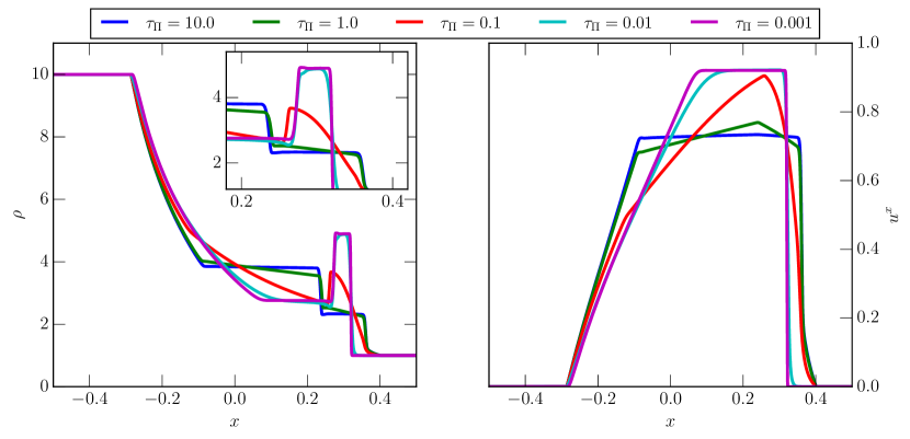
In this test we investigate the impact of bulk viscosity on a one-dimensional relativistic shocktube problem, see also Ref. Chabanov et al. (2021) for a similar test. Following Radice and Rezzolla (2012), we adopt the following initial conditions for a one-dimensional blast wave launched into an ambient medium. We adopt a domain along the -axis . All primitive variables, including the dissipative sector, are initialized to zero. The only non-zero quantities are given separately for , and as follows :
| (134) | |||
| (135) |
The system is closed by adopting an equation of state with . In order to study the behavior of bulk viscous dissipation, we adopt a fixed and vary . This will allow us to probe the limit discussed in Sec. III.1.1 . All other dissipative coefficients are set to zero, i.e. with their corresponding relaxation timescales fixed to values smaller than the dynamical time of the problem, i.e. . With this choice, the system will only be subject to bulk viscous dissipation. The evolution of the baryon density and velocity is shown in Fig. 1 for different values of the bulk viscous relaxation time . We can anticipate that for this particular choice of the transport coefficients the code will converge to two limiting solutions, see Sec. III.1.1. In the case of (magenta curve), the effective timescale associated lengthscale of the bulk viscosity will be too small to affect the dynamics of the shock problem, which happens on scales . Hence, the solution will approach the perfect fluid solution. On the other hand, following the discussion in Sec. III.1.1, we approach a non-perfect fluid limit already in the case of , which changes the shock structure (blue curve in Fig. 1).
Intermediate values of the bulk viscosity, , on the other hand, have the ability to interpolate between the two limits. This transition can be best understood when looking at the velocity , where for increasing relaxation time the velocity profile transitions from the higher speed perfect fluid solution (magenta curve) to the advected solution (blue curve) at slightly lower velocities.
V.2 One-dimensional heat conduction
We proceed by analyzing the ability of the system to conduct heat in a one-dimensional test setup. In order to pick a suitable set of initial conditions, we recall that in the limit of , the system reduces to the Telegrapher’s equation (38). In the Navier-Stokes limit of we further recover,
| (136) |
which is the standard heat equation. The fundamental solution to this equation, i.e. starting from initial conditions , is a Gaussian,
| (137) |
Here, we have introduced the effective diffusion constant . While this solution only holds approximately in the limit of , the full solution of the Telegrapher’s equation for the above initial condition instead reads Romatschke (2010b),
| (138) |
where the Heaviside functions ensure causality of the solution. Here, is a modified Bessel function of the first kind. Motivated by these observations we initialize an initial temperature distribution to resemble a Gaussian in hydrostatic equilibrium, i.e.,
| (139) | |||
| (140) | |||
| (141) |
where we adopt .
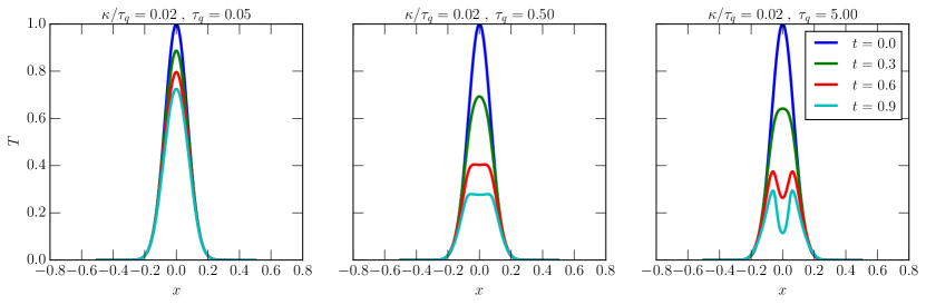
Our simulations use a grid resolution corresponding to grid points in the
interval . We then show the resulting profiles for different
times in Fig. 2. We can see that the evolution differs
drastically for fixed . For low and, hence,
fast relaxation (left panel), we can see that the initial Gaussian slowly
diffuses. On the other hand, for larger (center panel) the
diffusive process happens more rapidly but the Gaussian is eventually
flattening. For even larger relaxation time, , which is much larger than the dynamical
time scale of the simulation, we see that the wave part in the
Telegrapher’s equation (38) takes over and the Gaussian
begins to split apart. Hence, in this limit of large mean-free path the dynamics
is more similar to a damped wave equation than to a diffusion equation.
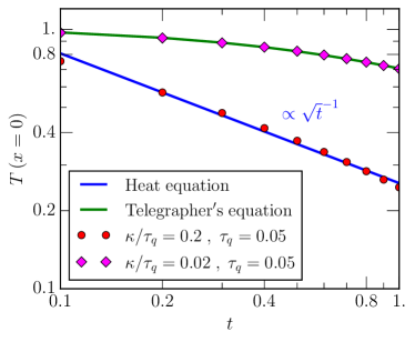
In order to assess whether we are indeed recovering the correct analytic solution of the Telegrapher’s (38) and Heat equations (136), we compare the evolution of the center point, with the analytic solutions (138) and (137). This comparison is shown in Fig. 3. We can see that for different choices of the transport coefficient the two limits can be reliably recovered. In particular, it is worth highlighting that causality, which limits the instantaneous spreading of heat, can significantly slow down dissipation compared to standard parabolic heat conduction, for which .
V.3 Two-dimensional heat conduction
We now continue to explore the effects of thermal conductivity in a two-dimensional setting. In particular, we follow a setup first proposed by Ref. Chandra et al. (2017),
| (142) | |||
| (143) | |||
| (144) | |||
| (145) |
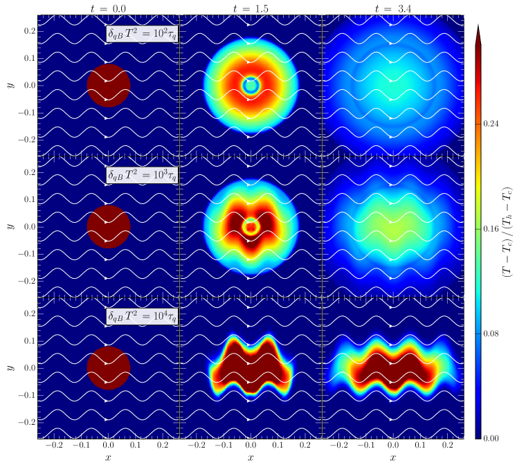
As before, all quantities not explicity listed have been initialized to zero. We emphasize that the initial condition is in pressure equilibrium and, in the absence of initial velocities, would remain static if dissipative effects were not present. Adopting an equation of state , this corresponds to an inner hot region with temperature and an outer cold region with temperature . In this problem, we explicitly include a global magnetic field to study the dependence with the gyrofrequency parameter . Inspired by the functional form of this parameter found for ultrarelativistic gases Denicol et al. (2019), we chose
| (147) | |||
| (148) | |||
| (149) |
The evolution for different values of is shown in Fig. 4. We can see that in the almost isotropic case, i.e. , heat conduction proceeds independently of the magnetic field geometry. More specifically, we can see in the middle and right panels of the first row in Fig. 4 that the temperature evolution retains its cylindrical symmetry. With increasing degree of anisotropy (middle row), we can see that the temperature evolution begins to be affected by the presence of the magnetic field. Physically, the increase in gyrofrequency beings to suppress cross-conductivity. In particular, the initially cylindrical temperature profile begins to split up (center panel) and heat conduction along the magnetic field starts to be enhanced. Comparing the final times (right column), we still find that the overall profile of the heat conduction is almost isotropic with only a small degree of anisotropy being present. Finally, by further increasing the degree of anisotropy , the heat flux begins to fully align with the magnetic field, i.e. , where the latter approximation is valid in the limit of small velocities. This is the limit of extended magnetohydrodynamics discussed in Sec. III.4.1.
We can see from the bottom row of Fig. 4 that in this limit heat conduction across the magnetic field lines is essentially absent and that the evolution is similar to the test case presented in Ref. Chandra et al. (2017). We note, however, that because the closure adopted in the present formulation allows to dynamically adjust the degree of anisotropy, we can naturally interpolate between the highly collisional (top row) and weakly collisional limits (bottom row).
V.4 Two-dimensional Kelvin-Helmholtz instability
Having discussed the behavior of bulk viscosity and heat conductivity in a series of numerical tests, we now turn to the effect of shear viscosity. In particular, we focus on a standard test problem routinely studied in the context of the Newtonian Navier-Stokes equations Lecoanet et al. (2016). Adopting the initial conditions presented in Beckwith and Stone (2011), we study the formation of vortices in a two-dimensional Kelvin-Helmholtz unstable shear layer. More precisely, we use
| (150) | |||
| (151) | |||
| (152) | |||
| (153) |
where we have further adopted . As before, all quantities not listed above have been initialized to zero. For this test problem we include both shear viscosity and heat conduction by fixing
| (154) | |||
| (155) | |||
| (156) | |||
| (157) |
which gives rise to an effective thermal Prandtl number .
Shear stresses act in providing a fixed cut-off for small scale turbulence, which is set by the length scale of the shear viscosity , where is a characteristic velocity scale. If instead of an explicit viscosity this cut-off was solely provided by the grid scale, i.e. , the outcome of the simulation would strongly depend on the given resolution. Hence, demonstrating resolved and converged vortex formation in a Kelvin-Helmholtz unstable shear layer has become a standard test problem for non-relativistic hydrodynamics Lecoanet et al. (2016). Following the same logic, we will perform simulations at three different resolutions, labeled by the number of grid points , where .
In order to establish a baseline for the effect of underresolved shear viscosity, we perform a first set of simulations for . The resulting baryon density evolution during vortex formation is shown in Fig. 5. Comparing the lowest (left panel) and highest resolutions (right panel), we clearly find differences in the small scale evolution, particularly inside the vortex. The presence of grid dependent effective viscosity can best be appreciated by comparing the medium (middle panel) and high (right panel) resolution cases. While on first glance the density distributions look very similar, one can clearly spot the presence of secondary vortices being formed in the shear layers of the primary vortex. If the shear viscosity was instead constant and resolved by the numerical resolution, we would expect convergent behavior in the vortex evolution. That is, getting the same vortex above a certain sufficiently resolved resolution.
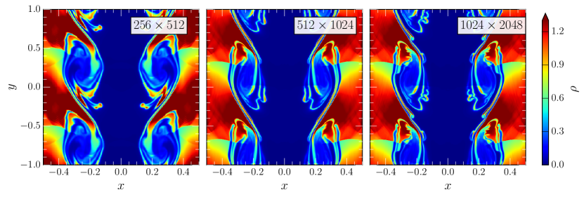
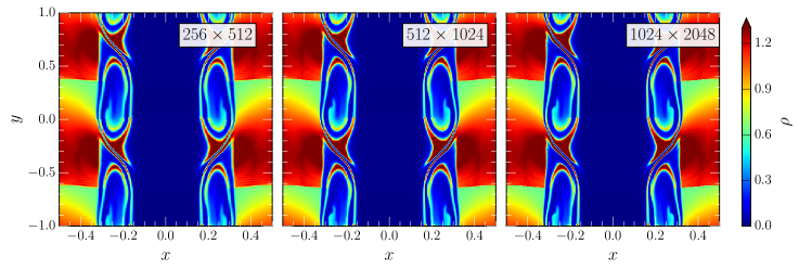
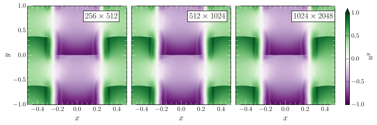
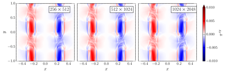
To demonstrate that this is indeed the case when using our viscous scheme, we perform the same simulation, but with the shear viscosity given by Eq. (157). The resulting evolutions for the baryon density , the velocity component along the shear layer, and the shear stresses and are shown in Fig. 6. Comparing the density evolutions with those shown in Fig. 5, the effect of a resolved shear viscosity is strikingly obvious. The formation of secondary vortices is suppressed at all resolutions and the vortices have the same internal structure in all cases, establishing that the relativistic form of the shear viscosity in flux-conservative form is working as expected. To better illustrate the dynamics, we next focus on the velocity along the shear layer (second row in Fig. 6). We can indeed see that relativistic velocities are present in the vortices. Furthermore we can see that strong shock fronts propagate through the vortices along the shear layer, coinciding with the jump (red to green color) in the rest-mass density . Looking at the shear stresses (third row in Fig. 6), we can see that the shear stresses are perfectly resolved and converged at all resolutions, with the strongest stresses present inside the vortices, as expected.
The most remarkable feature of our numerical simulations now arise in the bottom panel of Fig. 6. Since these simulations do not include explicit bulk viscosity, i.e. , the strong shock fronts propagating along the shear layer are not resolved and should manifest almost as discontinuities, similar to the shock tube solutions for perfect fluids shown in Fig. 1. Taking as a proxy for these stresses, we indeed find very sharp almost discontinuous jumps across the shocks, getting sharper when going from the lowest (left panel) to the highest (right panel) simulation. While handling such strong discontinuities might be difficult with more traditional finite-difference approaches to the shear stresses Del Zanna et al. (2013); Bazow et al. (2018), our way of incorporating the first-order dissipative forms in flux-conservative form clearly allows us to perfectly handle those steep jumps using high-resolution shock capturing methods.
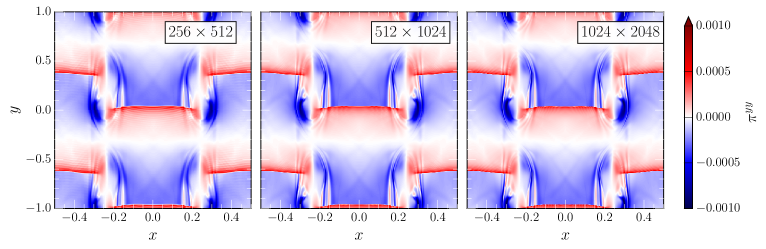
V.5 Two-dimensional Kelvin-Helmholtz instability in the presence of magnetic fields
As a final test, we investigate the weakly collisional regime when
shear stresses and heat fluxes are included. As discussed in Sec. III.4.1, in the limit of large mean-free-path the couplings
and diverge, leading to the heat flux and
shear stresses to align with the co-moving magnetic field.
In the case of globally sheared accretion flows,
hybrid-kinetic simulations of shearing flows in accretion disks
have shown that in this limit
mirror and firehose instabilities lead to a local enhancement of
collisionality Kunz et al. (2016). These instabilities are expected to kick in, once
Foucart et al. (2016)
| (158) | |||
| (159) |
Additionally, the heat flux is expected to be bound Cowie and McKee (1977); Foucart et al. (2016),
| (160) |
where is the sound speed in the fluid. Once these instabilities are triggered they lead to a local enhancement of collisionality and effectively pin the stresses at the threshold values for the instability. Within the framework of dissipative hydrodynamics, this can most easily be incorporated by locally adjusting the relaxation time , while keeping the ratios of the transport coefficients fixed, i.e. .
To do this, we adjust the relaxation times during the implicit solve of Eq. (112) and (113). We then consider the same setup presented in Sec. V.4, but add a uniform magnetic field
| (161) |
while keeping the other magnetic field components at zero initially. This results in an initial plasma parameter , for which the magnetic field in itself is not dynamically important. That is, in the absence of magnetic field induced anisotropies of heat fluxes and shear stresses, the simulation outcome will not differ from a purely hydrodynamical simulation. However, because of the anisotropic coupling with the magnetic field, the differences observed between the simulations will be purely because of the anisotropic nature of the dissipative variables. Furthermore, for such a choice of the mirror and firehose instability are expected to quench any anisotropy of the shear stresses.
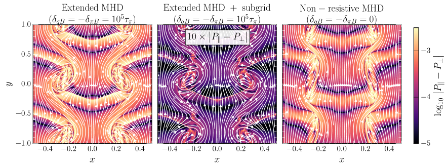
We present the result of these simulations in Fig. 7 at time . Specifically, we consider the case of , in which the equations approach the Braginskii-like limit of extended magnetohydrodynamics Chandra et al. (2015). We also consider the same parameters, but supplemented with the subgrid model discussed above. Starting from the top, we show the pressure anisotropy , where and are the pressures along and perpendicular to the magnetic field. The scalar was defined in Eq. (53). We can see that the global magnetic field evolution is very similar in all cases, except in the absence of the magnetic field coupling , in which the vortices are much more collapsed (right panel). In the limit of extended magnetohydrodynamics the vortices are much more circular, although there are differences within the vortex, when comparing the purely extended magnetohydrodynamics case (left panel) with the subgrid modeling (middle panel). Most importantly, we can see that the shear stresses are highly anisotropic, especially in the case of extended magnetohydrodynamics (left). However, as expected from the firehose and mirror instabilities, the effective subgrid model eliminates this anisotropy almost entirely with the pressure anisotropy being about a 100-times smaller (middle panel).
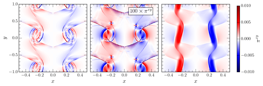
In the middle row, we show the -component of the shear stress tensor . Starting from the limit of extended magnetohydrodynamics with subgrid model (middle panel), we can see that the shear-stresses overall are times weaker than in the other cases, as expected from the discussion of above. Looking at the case of pure Extended magnetohydrodynamics (left panel), we can also see that small-scale substructures are present inside the vortices. Comparing the the structures in the magnetic field (top row), we can clearly see that shear stresses nicely align with the magnetic field geometry. When comparing with the case without the coupling (right panel), we can see that the stresses are uniformly present inside the vortices, where strongest shear flows are present. As expected for an enhancement of collisionality, the simulation including the subgrid model locally suppresses the shear stresses inside the vortices. The disappearance of substructure in the main vortices is also broadly consistent with the outcome of a similar Newtonian simulation assessing the impact of the subgrid model Berlok et al. (2020). Since the shear stresses are very small in this case, they might not be able to perfectly suppress the formation of secondary vortices, as in the isotropic viscous case, see Fig. 6. Indeed we see the (re-)appearance of secondary vortices when adding the sugrid model (middel panel).
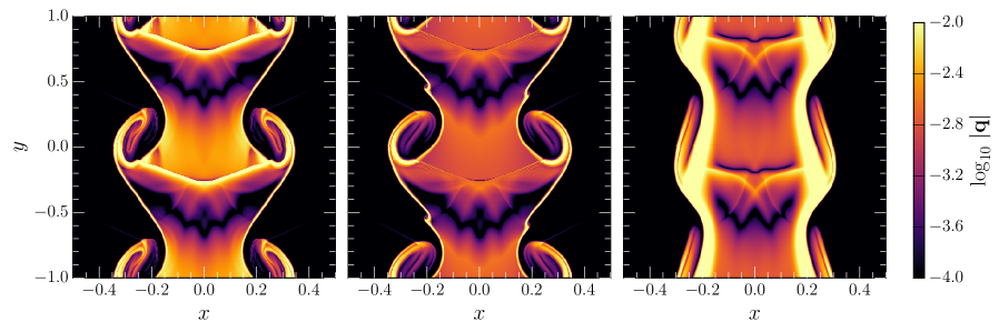
Finally, we turn to the heat flux present in these simulations, which is shown in the bottom row of Fig. 7. We can see that in the case without magnetic field coupling (right panel), a strong heat flux is present along the shear layer. This heat flux is able to diffuse the part of the pressure support of the vortices helping the collapse of the vortex compared to the extended magnetohydrodynamics cases (left and center panels). Since for those the heat flux has to align with the magnetic field, no heat conduction across the shear layer can happen, as the magnetic field is aligned with the layer so that the vortices will retain an additional pressure support. Moreover, when considering the shock that propagates along the interface, we can see that in the unlimited case (left panel) a strong heat flux is present that travels with the shock. In the case of the subgrid model, where the heat flux is clamped, see Eq. (160), the transport of heat is suppressed as these low density regions do not permit strong heat fluxes.
VI Conclusions
In this work, we have presented a new formulation to numerically model relativitic dissipative effects in the presence of magnetic fields. More specifically, starting from a collisional 14-moment closure Denicol et al. (2012) for non-resistive relativistic magnetohydrodynamics Denicol et al. (2018), we have derived a set of equations suitable for the study of heat conduction as well as bulk and shear viscosities in an astrophysical context. By treating the fluid frame projector implicitly we were able to recast the equations in fully flux conservative form. Different from earlier approaches (e.g. Del Zanna et al. (2013); Bazow et al. (2018)), this allows us to treat all dissipative variables using high-resolution shock capturing methods, which removes any ambiguities of how to compute either explicit time or spatial derivatives in the dissipative sources.
In addition, the numerical scheme includes two coupling terms that project the shear stresses and heat flux onto the comoving magnetic fields. This coupling has been identified with the gyrofrequency, allowing us for the first time to fully include this effect in a relativistic magnetohydrodynamics simulations. We have further demonstrated that for large coupling the system approaches the relativistic Braginskii-like limit of extended magnetohydrodynamics investigated in Ref. Chandra et al. (2015). This allows us to study effects of weakly collisional plasmas that could be relevant for certain types of black hole accretion Foucart et al. (2016, 2017).
To investigate the properties of the solutions of the equations of motion, we have also presented a set of numerical simulations aimed at testing each of the dissipative effects individually. In particular, we have considered one- and two-dimensional tests of heat conduction and viscous shear flows in flat-spacetime. Our results showed that all effects can be correctly captured with or without (coupled) magnetic fields being present. As such, we expect that this scheme will be highly suitable to numerically study highly relativistic magnetohydrodynamical turbulence Zrake and MacFadyen (2012, 2013), black hole accretion Foucart et al. (2016), and dissipative effects in neutron star mergers Shibata et al. (2017); Alford et al. (2018); Most et al. (2021); Hammond et al. (2021).
An important aspect not yet addressed in this work are causality bounds on the system presented here. While conditions that ensure causality in the nonlinear regime of Israel-Stewart-like equations formulated in the Landau frame (in the absence of magnetic fields or baryon density) have been derived in Bemfica et al. (2021) (and strong hyperbolicity has been proven in Bemfica et al. (2019a) in the case of only bulk viscosity), no such conditions exist either when magnetic fields are included, or for the equations presented here, which have additional relaxation equations. Although our equations do approach standard Israel-Stewart-like equations in the stiff limit, we currently have no proof under which conditions the equations presented here maintain causality in the nonlinear regime (the linear regime of the theory derived in Denicol et al. (2018) was investigated in Biswas et al. (2020)). Such an analysis will have to be performed for our system as well, although our ability to solve this system in a stable manner under all conditions investigated here provides an optimistic indication that causality and hyperbolicity can be established in this system 333We stress at this point that a flux-conservative treatment requires the specification of an upper-limit of the system of characteristics, which we approximate with the speed of light. If the actual characteristics were much larger, the system would loose its upwind properties leading to numerical instabilities..
Beyond our current approach, several extensions are possible, in particular when considering applications to the hydrodynamic evolution of the quark-gluon plasma Romatschke and Romatschke (2019). In that regard, the next step would be to check how our framework handles Gubser flow Gubser (2010), which has become the standard test for numerical codes in the field of heavy-ion collisions Marrochio et al. (2015). In fact, when considering heavy-ion applications, we would have to also incorporate second-order coupling terms Denicol et al. (2012), though the effects of some of those terms on causality are not yet known in the nonlinear regime even at zero baryon chemical potential (for instance, Ref. Bemfica et al. (2021) neglected terms involving the coupling between the vorticity tensor and the shear stress tensor).
Furthermore, we have limited ourselves to non-resistive plasmas. A natural
extension we are planning is the incorporation of resistivity effects,
which have been investigated in Denicol et al. (2019). Extrapolating our
results, this will allow us to correctly treat the relativistic Hall effect
Zanotti and Dumbser (2011) and relativistic reconnection
Bransgrove et al. (2021), which could be highly relevant for flaring
process around accreting supermassive black holes
Nathanail et al. (2020); Ripperda et al. (2020).
Acknowledgements
The authors thank Lev Arzamasskiy, Fabio Bemfica, Amitava Bhattarcharjee, Mani Chandra, Gabriel Denicol, Marcelo Disconzi, Charles Gammie, James Juno, Alex Pandya, Frans Pretorius, Alexander
Philippov, Bart Ripperda and James Stone for insightful discussions and
comments related to this work.
ERM gratefully acknowledges support from postdoctoral fellowships
at the Princeton Center for Theoretical Science, the Princeton
Gravity Initiative, and the Institute for Advanced Study.
JN is partially supported by the U.S. Department of Energy, Office of Science, Office for Nuclear Physics under Award No. DE-SC0021301.
All simulations were performed on the Helios Cluster at the Institute for Advanced Study.
References
- Romatschke and Romatschke (2019) P. Romatschke and U. Romatschke, Relativistic Fluid Dynamics In and Out of Equilibrium, Cambridge Monographs on Mathematical Physics (Cambridge University Press, 2019) arXiv:1712.05815 [nucl-th] .
- Weinberg (2008) S. Weinberg, Cosmology (2008).
- Baiotti and Rezzolla (2017) L. Baiotti and L. Rezzolla, Rept. Prog. Phys. 80, 096901 (2017), arXiv:1607.03540 [gr-qc] .
- Heinz and Snellings (2013) U. Heinz and R. Snellings, Ann. Rev. Nucl. Part. Sci. 63, 123 (2013), arXiv:1301.2826 [nucl-th] .
- Bernhard et al. (2019) J. E. Bernhard, J. S. Moreland, and S. A. Bass, Nature Phys. 15, 1113 (2019).
- Nijs et al. (2021) G. Nijs, W. van der Schee, U. Gürsoy, and R. Snellings, Phys. Rev. C 103, 054909 (2021), arXiv:2010.15134 [nucl-th] .
- Everett et al. (2021a) D. Everett et al. (JETSCAPE), Phys. Rev. Lett. 126, 242301 (2021a), arXiv:2010.03928 [hep-ph] .
- Everett et al. (2021b) D. Everett et al. (JETSCAPE), Phys. Rev. C 103, 054904 (2021b), arXiv:2011.01430 [hep-ph] .
- Israel and Stewart (1979) W. Israel and J. M. Stewart, Annals Phys. 118, 341 (1979).
- Baier et al. (2008) R. Baier, P. Romatschke, D. T. Son, A. O. Starinets, and M. A. Stephanov, JHEP 04, 100 (2008), arXiv:0712.2451 [hep-th] .
- Denicol et al. (2012) G. S. Denicol, H. Niemi, E. Molnar, and D. H. Rischke, Phys. Rev. D 85, 114047 (2012), [Erratum: Phys.Rev.D 91, 039902 (2015)], arXiv:1202.4551 [nucl-th] .
- Martinez and Strickland (2010) M. Martinez and M. Strickland, Nucl. Phys. A 848, 183 (2010), arXiv:1007.0889 [nucl-th] .
- Florkowski and Ryblewski (2011) W. Florkowski and R. Ryblewski, Phys. Rev. C 83, 034907 (2011), arXiv:1007.0130 [nucl-th] .
- Bazow et al. (2014) D. Bazow, U. W. Heinz, and M. Strickland, Phys. Rev. C 90, 054910 (2014), arXiv:1311.6720 [nucl-th] .
- Alqahtani et al. (2018) M. Alqahtani, M. Nopoush, and M. Strickland, Prog. Part. Nucl. Phys. 101, 204 (2018), arXiv:1712.03282 [nucl-th] .
- Alqahtani et al. (2017) M. Alqahtani, M. Nopoush, R. Ryblewski, and M. Strickland, Phys. Rev. Lett. 119, 042301 (2017), arXiv:1703.05808 [nucl-th] .
- Hiscock and Lindblom (1983) W. A. Hiscock and L. Lindblom, Annals Phys. 151, 466 (1983).
- Olson (1990) T. S. Olson, Annals Phys. 199, 18 (1990).
- Bemfica et al. (2019a) F. S. Bemfica, M. M. Disconzi, and J. Noronha, Phys. Rev. Lett. 122, 221602 (2019a), arXiv:1901.06701 [gr-qc] .
- Bemfica et al. (2021) F. S. Bemfica, M. M. Disconzi, V. Hoang, J. Noronha, and M. Radosz, Phys. Rev. Lett. 126, 222301 (2021), arXiv:2005.11632 [hep-th] .
- Chiu and Shen (2021) C. Chiu and C. Shen, Phys. Rev. C 103, 064901 (2021), arXiv:2103.09848 [nucl-th] .
- Plumberg et al. (2021) C. Plumberg, D. Almaalol, T. Dore, J. Noronha, and J. Noronha-Hostler, (2021), arXiv:2103.15889 [nucl-th] .
- Romatschke and Romatschke (2007) P. Romatschke and U. Romatschke, Phys. Rev. Lett. 99, 172301 (2007), arXiv:0706.1522 [nucl-th] .
- Schenke et al. (2012) B. Schenke, S. Jeon, and C. Gale, Phys. Rev. C 85, 024901 (2012), arXiv:1109.6289 [hep-ph] .
- Bozek (2012) P. Bozek, Phys. Rev. C 85, 034901 (2012), arXiv:1110.6742 [nucl-th] .
- Del Zanna et al. (2013) L. Del Zanna, V. Chandra, G. Inghirami, V. Rolando, A. Beraudo, A. De Pace, G. Pagliara, A. Drago, and F. Becattini, Eur. Phys. J. C 73, 2524 (2013), arXiv:1305.7052 [nucl-th] .
- Karpenko et al. (2014) I. Karpenko, P. Huovinen, and M. Bleicher, Comput. Phys. Commun. 185, 3016 (2014), arXiv:1312.4160 [nucl-th] .
- Shen et al. (2016) C. Shen, Z. Qiu, H. Song, J. Bernhard, S. Bass, and U. Heinz, Comput. Phys. Commun. 199, 61 (2016), arXiv:1409.8164 [nucl-th] .
- Habich et al. (2015) M. Habich, J. L. Nagle, and P. Romatschke, Eur. Phys. J. C 75, 15 (2015), arXiv:1409.0040 [nucl-th] .
- Romatschke (2015) P. Romatschke, Eur. Phys. J. C 75, 305 (2015), arXiv:1502.04745 [nucl-th] .
- Bazow et al. (2018) D. Bazow, U. W. Heinz, and M. Strickland, Comput. Phys. Commun. 225, 92 (2018), arXiv:1608.06577 [physics.comp-ph] .
- Okamoto and Nonaka (2017) K. Okamoto and C. Nonaka, Eur. Phys. J. C 77, 383 (2017), arXiv:1703.01473 [nucl-th] .
- Noronha-Hostler et al. (2013) J. Noronha-Hostler, G. S. Denicol, J. Noronha, R. P. G. Andrade, and F. Grassi, Phys. Rev. C 88, 044916 (2013), arXiv:1305.1981 [nucl-th] .
- Noronha-Hostler et al. (2014) J. Noronha-Hostler, J. Noronha, and F. Grassi, Phys. Rev. C 90, 034907 (2014), arXiv:1406.3333 [nucl-th] .
- Noronha-Hostler et al. (2016) J. Noronha-Hostler, J. Noronha, and M. Gyulassy, Phys. Rev. C 93, 024909 (2016), arXiv:1508.02455 [nucl-th] .
- Jeon and Heinz (2015) S. Jeon and U. Heinz, Int. J. Mod. Phys. E 24, 1530010 (2015), arXiv:1503.03931 [hep-ph] .
- Monaghan (1992) J. J. Monaghan, Ann. Rev. Astron. Astrophys. 30, 543 (1992).
- Aguiar et al. (2001) C. E. Aguiar, T. Kodama, T. Osada, and Y. Hama, J. Phys. G 27, 75 (2001), arXiv:hep-ph/0006239 .
- Shakura and Sunyaev (1973) N. I. Shakura and R. A. Sunyaev, Astron. & Astrophys. 500, 33 (1973).
- Alford et al. (2018) M. G. Alford, L. Bovard, M. Hanauske, L. Rezzolla, and K. Schwenzer, Phys. Rev. Lett. 120, 041101 (2018), arXiv:1707.09475 [gr-qc] .
- Most et al. (2021) E. R. Most, S. P. Harris, C. Plumberg, M. G. Alford, J. Noronha, J. Noronha-Hostler, F. Pretorius, H. Witek, and N. Yunes, (2021), arXiv:2107.05094 [astro-ph.HE] .
- Radice (2017) D. Radice, Astrophys. J. Lett. 838, L2 (2017), arXiv:1703.02046 [astro-ph.HE] .
- Fujibayashi et al. (2018) S. Fujibayashi, K. Kiuchi, N. Nishimura, Y. Sekiguchi, and M. Shibata, Astrophys. J. 860, 64 (2018), arXiv:1711.02093 [astro-ph.HE] .
- Shibata et al. (2017) M. Shibata, K. Kiuchi, and Y.-i. Sekiguchi, Phys. Rev. D 95, 083005 (2017), arXiv:1703.10303 [astro-ph.HE] .
- Fujibayashi et al. (2020) S. Fujibayashi, M. Shibata, S. Wanajo, K. Kiuchi, K. Kyutoku, and Y. Sekiguchi, Phys. Rev. D 101, 083029 (2020), arXiv:2001.04467 [astro-ph.HE] .
- Price and Rosswog (2006) D. Price and S. Rosswog, Science 312, 719 (2006), arXiv:astro-ph/0603845 .
- Kiuchi et al. (2015) K. Kiuchi, P. Cerdá-Durán, K. Kyutoku, Y. Sekiguchi, and M. Shibata, Phys. Rev. D 92, 124034 (2015), arXiv:1509.09205 [astro-ph.HE] .
- Aguilera-Miret et al. (2020) R. Aguilera-Miret, D. Viganò, F. Carrasco, B. Miñano, and C. Palenzuela, Phys. Rev. D 102, 103006 (2020), arXiv:2009.06669 [gr-qc] .
- Skoutnev et al. (2021) V. Skoutnev, E. R. Most, A. Bhattacharjee, and A. A. Philippov, (2021), arXiv:2106.04787 [physics.flu-dyn] .
- Hiscock and Lindblom (1985) W. A. Hiscock and L. Lindblom, Phys. Rev. D 31, 725 (1985).
- Duez et al. (2004) M. D. Duez, Y. T. Liu, S. L. Shapiro, and B. C. Stephens, Phys. Rev. D 69, 104030 (2004), arXiv:astro-ph/0402502 .
- Fragile et al. (2018) P. C. Fragile, S. M. Etheridge, P. Anninos, B. Mishra, and W. Kluzniak, Astrophys. J. 857, 1 (2018), arXiv:1803.06423 [astro-ph.HE] .
- Chabanov et al. (2021) M. Chabanov, L. Rezzolla, and D. H. Rischke, Mon. Not. Roy. Astron. Soc. 505, 5910 (2021), arXiv:2102.10419 [gr-qc] .
- Bemfica et al. (2018) F. S. Bemfica, M. M. Disconzi, and J. Noronha, Phys. Rev. D 98, 104064 (2018), arXiv:1708.06255 [gr-qc] .
- Kovtun (2019) P. Kovtun, JHEP 10, 034 (2019), arXiv:1907.08191 [hep-th] .
- Bemfica et al. (2019b) F. S. Bemfica, M. M. Disconzi, and J. Noronha, Phys. Rev. D 100, 104020 (2019b), arXiv:1907.12695 [gr-qc] .
- Hoult and Kovtun (2020) R. E. Hoult and P. Kovtun, JHEP 06, 067 (2020), arXiv:2004.04102 [hep-th] .
- Bemfica et al. (2020) F. S. Bemfica, M. M. Disconzi, and J. Noronha, (2020), arXiv:2009.11388 [gr-qc] .
- Pandya and Pretorius (2021) A. Pandya and F. Pretorius, Phys. Rev. D 104, 023015 (2021), arXiv:2104.00804 [gr-qc] .
- Peshkov et al. (2019) I. Peshkov, E. Romenski, F. Fambri, and M. Dumbser, (2019), arXiv:1910.02687 [gr-qc] .
- Romenski et al. (2020) E. Romenski, I. Peshkov, M. Dumbser, and F. Fambri, Phil. Trans. Roy. Soc. Lond. A 378, 20190175 (2020), arXiv:1910.03298 [gr-qc] .
- Radice (2020) D. Radice, Symmetry 12, 1249 (2020), arXiv:2005.09002 [astro-ph.HE] .
- Duez et al. (2020) M. D. Duez, A. Knight, F. Foucart, M. Haddadi, J. Jesse, F. Hebert, L. E. Kidder, H. P. Pfeiffer, and M. A. Scheel, Phys. Rev. D 102, 104050 (2020), arXiv:2008.05019 [gr-qc] .
- Denicol et al. (2018) G. S. Denicol, X.-G. Huang, E. Molnár, G. M. Monteiro, H. Niemi, J. Noronha, D. H. Rischke, and Q. Wang, Phys. Rev. D 98, 076009 (2018), arXiv:1804.05210 [nucl-th] .
- Denicol et al. (2019) G. S. Denicol, E. Molnár, H. Niemi, and D. H. Rischke, Phys. Rev. D 99, 056017 (2019), arXiv:1902.01699 [nucl-th] .
- Panda et al. (2021) A. K. Panda, A. Dash, R. Biswas, and V. Roy, JHEP 03, 216 (2021), arXiv:2011.01606 [nucl-th] .
- Toro (2013) E. F. Toro, Riemann solvers and numerical methods for fluid dynamics: a practical introduction (Springer Science & Business Media, 2013).
- Pareschi and Russo (2005) L. Pareschi and G. Russo, Journal of Scientific computing 25, 129 (2005).
- Alic et al. (2012) D. Alic, P. Mosta, L. Rezzolla, O. Zanotti, and J. L. Jaramillo, Astrophys. J. 754, 36 (2012), arXiv:1204.2226 [gr-qc] .
- Palenzuela (2013) C. Palenzuela, Mon. Not. Roy. Astron. Soc. 431, 1853 (2013), arXiv:1212.0130 [astro-ph.HE] .
- Most and Philippov (2020) E. R. Most and A. A. Philippov, Astrophys. J. Lett. 893, L6 (2020), arXiv:2001.06037 [astro-ph.HE] .
- Duez et al. (2005) M. D. Duez, Y. T. Liu, S. L. Shapiro, and B. C. Stephens, Phys. Rev. D 72, 024028 (2005), arXiv:astro-ph/0503420 .
- Eckart (1940) C. Eckart, Phys. Rev. 58, 919 (1940).
- Tsumura and Kunihiro (2010) K. Tsumura and T. Kunihiro, Phys. Lett. B 690, 255 (2010), arXiv:0906.0079 [hep-ph] .
- Noronha et al. (2021) J. Noronha, M. Spaliński, and E. Speranza, (2021), arXiv:2105.01034 [nucl-th] .
- Rocha and Denicol (2021) G. S. Rocha and G. S. Denicol, (2021), arXiv:2108.02187 [nucl-th] .
- Landau and Lifshitz (1987) L. D. Landau and E. M. Lifshitz, Fluid Mechanics - Volume 6 (Course of Theoretical Physics), 2nd ed. (Butterworth-Heinemann, 1987) p. 552.
- Pichon (1965) G. Pichon, Ann. Inst. H. Poincaré Sect. A (N.S.) 2, 21 (1965).
- Biswas et al. (2020) R. Biswas, A. Dash, N. Haque, S. Pu, and V. Roy, JHEP 10, 171 (2020), arXiv:2007.05431 [nucl-th] .
- Rezzolla and Zanotti (2013) L. Rezzolla and O. Zanotti, Relativistic hydrodynamics (Oxford University Press, 2013).
- Oertel et al. (2017) M. Oertel, M. Hempel, T. Klähn, and S. Typel, Rev. Mod. Phys. 89, 015007 (2017), arXiv:1610.03361 [astro-ph.HE] .
- Romatschke (2010a) P. Romatschke, Class. Quant. Grav. 27, 025006 (2010a), arXiv:0906.4787 [hep-th] .
- Sturrock and Andrew (1994) P. Sturrock and S. Andrew, Plasma Physics: An Introduction to the Theory of Astrophysical, Geophysical and Laboratory Plasmas, Stanford-Cambridge program (Cambridge University Press, 1994).
- Braginskii (1965) S. Braginskii, Reviews of plasma physics 1 (1965).
- Chandra et al. (2015) M. Chandra, C. F. Gammie, F. Foucart, and E. Quataert, Astrophys. J. 810, 162 (2015), arXiv:1508.00878 [astro-ph.HE] .
- Foucart et al. (2016) F. Foucart, M. Chandra, C. F. Gammie, and E. Quataert, Mon. Not. Roy. Astron. Soc. 456, 1332 (2016), arXiv:1511.04445 [astro-ph.HE] .
- Foucart et al. (2017) F. Foucart, M. Chandra, C. F. Gammie, E. Quataert, and A. Tchekhovskoy, Mon. Not. Roy. Astron. Soc. 470, 2240 (2017), arXiv:1706.01533 [astro-ph.HE] .
- Borges et al. (2008) R. Borges, M. Carmona, B. Costa, and W. S. Don, Journal of Computational Physics 227, 3191 (2008).
- Dionysopoulou et al. (2013) K. Dionysopoulou, D. Alic, C. Palenzuela, L. Rezzolla, and B. Giacomazzo, Phys. Rev. D 88, 044020 (2013), arXiv:1208.3487 [gr-qc] .
- Ripperda et al. (2019) B. Ripperda, F. Bacchini, O. Porth, E. R. Most, H. Olivares, A. Nathanail, L. Rezzolla, J. Teunissen, and R. Keppens, Astrophys. J. Suppl. 244, 10 (2019), arXiv:1907.07197 [physics.comp-ph] .
- Del Zanna et al. (2007) L. Del Zanna, O. Zanotti, N. Bucciantini, and P. Londrillo, Astron. Astrophys. 473, 11 (2007), arXiv:0704.3206 [astro-ph] .
- McCorquodale and Colella (2011) P. McCorquodale and P. Colella, Communications in Applied Mathematics and Computational Science 6, 1 (2011).
- Most et al. (2019) E. R. Most, L. J. Papenfort, and L. Rezzolla, Mon. Not. Roy. Astron. Soc. 490, 3588 (2019), arXiv:1907.10328 [astro-ph.HE] .
- Felker and Stone (2018) K. G. Felker and J. M. Stone, Journal of Computational Physics 375, 1365 (2018), arXiv:1711.07439 [astro-ph.IM] .
- Stone et al. (2020) J. M. Stone, K. Tomida, C. J. White, and K. G. Felker, ApJS 249, 4 (2020), arXiv:2005.06651 [astro-ph.IM] .
- Edwards et al. (2014) H. C. Edwards, C. R. Trott, and D. Sunderland, Journal of Parallel and Distributed Computing 74, 3202 (2014), domain-Specific Languages and High-Level Frameworks for High-Performance Computing.
- Noble et al. (2006) S. C. Noble, C. F. Gammie, J. C. McKinney, and L. Del Zanna, Astrophys. J. 641, 626 (2006), arXiv:astro-ph/0512420 .
- Galeazzi et al. (2013) F. Galeazzi, W. Kastaun, L. Rezzolla, and J. A. Font, Phys. Rev. D 88, 064009 (2013), arXiv:1306.4953 [gr-qc] .
- Newman and Hamlin (2014) W. I. Newman and N. D. Hamlin, SIAM Journal on Scientific Computing 36, B661 (2014).
- Siegel et al. (2018) D. M. Siegel, P. Mösta, D. Desai, and S. Wu, Astrophys. J. 859, 71 (2018), arXiv:1712.07538 [astro-ph.HE] .
- Kastaun et al. (2021) W. Kastaun, J. V. Kalinani, and R. Ciolfi, Phys. Rev. D 103, 023018 (2021), arXiv:2005.01821 [gr-qc] .
- Broyden (1965) C. G. Broyden, Mathematics of computation 19, 577 (1965).
- Kelley (1995) C. T. Kelley, Iterative methods for linear and nonlinear equations (SIAM, 1995).
- Radice and Rezzolla (2012) D. Radice and L. Rezzolla, Astron. Astrophys. 547, A26 (2012), arXiv:1206.6502 [astro-ph.IM] .
- Romatschke (2010b) P. Romatschke, Int. J. Mod. Phys. E 19, 1 (2010b), arXiv:0902.3663 [hep-ph] .
- Chandra et al. (2017) M. Chandra, F. Foucart, and C. F. Gammie, Astrophys. J. 837, 92 (2017), arXiv:1702.01106 [astro-ph.IM] .
- Lecoanet et al. (2016) D. Lecoanet, M. McCourt, E. Quataert, K. J. Burns, G. M. Vasil, J. S. Oishi, B. P. Brown, J. M. Stone, and R. M. O’Leary, MNRAS 455, 4274 (2016), arXiv:1509.03630 [astro-ph.IM] .
- Beckwith and Stone (2011) K. Beckwith and J. M. Stone, Astrophys. J. Suppl. 193, 6 (2011), arXiv:1101.3573 [astro-ph.HE] .
- Kunz et al. (2016) M. W. Kunz, J. M. Stone, and E. Quataert, Phys. Rev. Lett. 117, 235101 (2016), arXiv:1608.07911 [astro-ph.HE] .
- Cowie and McKee (1977) L. L. Cowie and C. F. McKee, ApJ 211, 135 (1977).
- Berlok et al. (2020) T. Berlok, R. Pakmor, and C. Pfrommer, Mon. Not. Roy. Astron. Soc. 491, 2919 (2020), arXiv:1911.05694 [astro-ph.CO] .
- Zrake and MacFadyen (2012) J. Zrake and A. MacFadyen, Astrophys. J. 744, 32 (2012), arXiv:1108.1991 [astro-ph.HE] .
- Zrake and MacFadyen (2013) J. Zrake and A. MacFadyen, Astrophys. J. Lett. 763, L12 (2013), arXiv:1210.4066 [astro-ph.HE] .
- Hammond et al. (2021) P. Hammond, I. Hawke, and N. Andersson, (2021), arXiv:2108.08649 [astro-ph.HE] .
- Gubser (2010) S. S. Gubser, Phys. Rev. D 82, 085027 (2010), arXiv:1006.0006 [hep-th] .
- Marrochio et al. (2015) H. Marrochio, J. Noronha, G. S. Denicol, M. Luzum, S. Jeon, and C. Gale, Phys. Rev. C 91, 014903 (2015), arXiv:1307.6130 [nucl-th] .
- Zanotti and Dumbser (2011) O. Zanotti and M. Dumbser, Mon. Not. Roy. Astron. Soc. 418, 1004 (2011), arXiv:1103.5924 [astro-ph.HE] .
- Bransgrove et al. (2021) A. Bransgrove, B. Ripperda, and A. Philippov, Phys. Rev. Lett. 127, 055101 (2021).
- Nathanail et al. (2020) A. Nathanail, C. M. Fromm, O. Porth, H. Olivares, Z. Younsi, Y. Mizuno, and L. Rezzolla, Mon. Not. Roy. Astron. Soc. 495, 1549 (2020), arXiv:2002.01777 [astro-ph.HE] .
- Ripperda et al. (2020) B. Ripperda, F. Bacchini, and A. Philippov, Astrophys. J. 900, 100 (2020), arXiv:2003.04330 [astro-ph.HE] .
Appendix A Non-resistive dissipative magnetohydrodynamics in flat spacetime
The numerical tests presented in this paper are performed in flat Minkowski spacetime, where . We can further introduce a magnetic field
| (162) |
as seen by a Eulerian observer. In terms of this magnetic field, the comoving field reads
| (163) |
The overall evolution equations of non-resistive dissipative magnetohydrodynamics in flat Minkowski spacetime are then given by
| (164) | |||
| (165) | |||
| (166) | |||
| (167) | |||
| (168) | |||
| (169) | |||
| (170) | |||
| (171) | |||
| (172) | |||
| (173) | |||
| (174) | |||
| (175) |