Dissociative electron attachment to sulfur dioxide : A theoretical approach
Abstract
In this present investigation, density functional theory (DFT) and natural bond orbital (NBO) calculations have been performed to understand experimental observations of dissociative electron attachment (DEA) to SO2. The molecular structure, fundamental vibrational frequencies with their corresponding intensities and molecular electrostatic potential (MEP) map, signifying the electron density contours, of SO2 and SO are interpreted from respective ground state optimized electronic structures calculated using DFT. The MEPs are then quantified and the second order perturbation energies for different oxygen lone pair (n) to and interactions of S-O bond orbitals have been calculated by carrying out NBO analysis and the results are investigated. The change in the electronic structure of the molecule after the attachment of a low-energy ( 15 eV) electron, thus forming a transient negative ion (TNI), can be interpreted from the and interactions. The results of the calculations are used to interpret the dissociative electron attachment process. The dissociation of the anion SO into negative and neutral fragments has been explained by interpreting the infrared (IR) spectrum and the different vibration modes. It could be observed that the dissociation of the anion SO into S- occurs as a result of simultaneous symmetric stretching and bending modes of the molecular anion. While the formation of O- and SO- occurs as a result of anti-symmetric stretching of the molecular anion. The calculated symmetries of the TNI state contributing to the first resonant peak at around 5.2 eV and second resonant peak at around 7.5 eV could be observed from time-dependent density functional theory (TD-DFT) calculations to be an A1 and a combination of A1+B2 states for the two resonant peaks, respectively. These findings strongly support our recent experimental observations for DEA to SO2 using the sophisticated velocity map imaging (VMI) technique [Jana and Nandi, Phys. Rev. A, 2018, 97, 042706].
1 Introduction
Sulfur dioxide is a bent molecule with O-S-O bond angle of 119.30 and S-O bond length of 143.1pm having a C2v symmetry with ground state configuration (7a1)2,(1a2)2,(4b2)2,(8a1)2 [1]. The presence of sulfur dioxide in starting from acid rain to natural volcanic sources, makes it one of the most important atmospheric molecules [2]. Recording the vibrational bands and molecular constants of SO2 from the infrared (IR) spectrum of the molecule using an infrared prism-grating spectrometer have been reported since the early 1950’s [3]. Robert et al. also reported IR the spectrum of anhydrous liquid sulfur dioxide and anhydrous liquid hydrogen fluoride using a Perkin-Elmer, Model 21, double beam recording infrared spectrometer [4]. Recently, in the year 2014, Zhu et al. reported density functional theory (DFT) and natural bond orbital (NBO) calculations to study the electronic structures and bonding interactions between sulfur dioxide molecule and ruthenium (II) atom in two ruthenium-SO2 adducts [5]. Using the molecular structure, vibrational spectra and molecular electrostatic potential to study large polyatomic molecules like metolazone using the Gaussian 03 program package can be observed in the literature [6]. Ab initio calculations to investigate the enhancement of halogen bonds by -hole and -hole interactions between two molecules containing halogen atom in one, and a negative site in another has been reported by Esrafili and Vakili where, molecular electrostatic potential (MEP) of isolated SO2 has been computed [7].
Study of low-energy ( 15 eV) electron attachment to SO2 has been a topic of interest since the early 1970’s. There have been many experimental studies reporting dissociative electron attachment (DEA) to SO2 [1, 8, 9, 10, 11, 12, 13]. Experiments on DEA to SO2 is known to produce two prominent resonant peaks at around 5.2 and 7.5 eV as explained by the following reaction:
| (1) |
where a low-energy electron gets attached to the SO2 molecule via a resonant capture forming SO. This complex SO, called the transient negative ion (TNI), then dissociates giving neutral and anionic fragments.
Experiments reporting electron attachment cross-section of the negative ion fragments produced from DEA to SO2 and also the corresponding kinetic energies of the fragments using different processes are abundant in the literature [10, 9, 12, 8, 11]. Although experiments reporting angular distribution of the fragments are scarce [14]. But theories reporting DEA to SO2 are very less in the literature [15, 1]. In the year 1996, Krishnakumar et al. using ab initio molecular orbital calculations and selection rules for dissociative electron attachment reported the first resonance between 4-5 eV to be due to and the second peak at around 7 eV to be due to negative ion resonant states [1]. Recently, Jana and Nandi reported DEA to SO2 using the sophisticated velocity map imaging (VMI) and identified the first resonance around 5.2 eV due to an and the second resonance around 7.5 eV due to a combination of + negative ion resonant states [13].
We report a theoretical and computational approach to find out the optimized ground state molecular structure of neutral SO2 molecule and its anionic part SO formed after the attachment of a low energy electron to the molecule using Gaussian 09 program package [16]. The density functional theory (DFT) calculation has been performed using the Becke 3LYP exchange-correlational functional containing the Slater exchange functional, Hartree-Fock and Becke’s 1988 gradient correction, along with the Lee-Yang-Parr functional with a aug-cc-pVQZ basis set to obtain a stable structure [17, 18, 19, 20, 21, 22]. The results of these calculations are then used to find out change in the ground state electronic structure of the molecule after the electron attachment. The electron density distribution is then visualized for the neutral SO2 molecule and the SO TNI with the help of the molecular electrostatic potential (MEP) map. The electron density distribution has been quantified with the help of natural bond orbital (NBO) analysis, followed by bond order calculation and Mulliken charge analysis. A vibration spectral analysis is then carried out using the computed infrared (IR) spectrum, to investigate different vibration modes of the TNI and hence identify the formation of different negative and neutral fragments given by Eqn. 1. The potential curves for the first two dissociation pathways of Eqn. 1 have also been plotted for the neutral parent molecule and the optimized ground state configuration of the TNI, by varying the O-O and S-O bond distances, respectively. Finally, a time-dependent density functional theory (TD-DFT) calculation has been performed to calculate the vertical excited state energies of SO TNI and thus identify the negative ion resonant states of the TNI involved in DEA to SO2 at the first and second resonant peaks.
2 Modeling of the molecule and density functional theory
Density functional theory (DFT) calculations to small polyatomic molecules is abundant in the literature. In the present work, ab initio electronic structure calculation using DFT has been performed to neutral SO2 and its anionic part SO using Gaussian 09 program package [16]. Quantum chemical calculations using DFT is an efficient tool in illuminating not only the electronic structure of the SO2 molecule, but also how the neutral molecule reacts to the incoming low-energy electron thus forming the TNI state. It is well known that the electronic structure of anions can be obtained using DFT [23]. First, the ground state geometries of SO2 and SO molecules were optimized using DFT with the Becke 3LYP exchange-correlational functional with a aug-cc-pVQZ basis set to obtain a stable structure. The ground state optimized energy for SO2 comes out to be -548.733 Hartree while the optimized energy for ground state of SO comes out to be -548.785 Hartree. Thus the optimized ground state energy of SO is 1.42 eV lower than the ground state optimized energy of the neutral molecule. This indicates that the adiabatic electron affinity of SO2 is positive and given by the difference value of 1.42 eV. This matches excellently with Grabowski et al. who measured the electron affinity of SO2 to be 1.10.1 eV using the flowing afterglow technique [24].
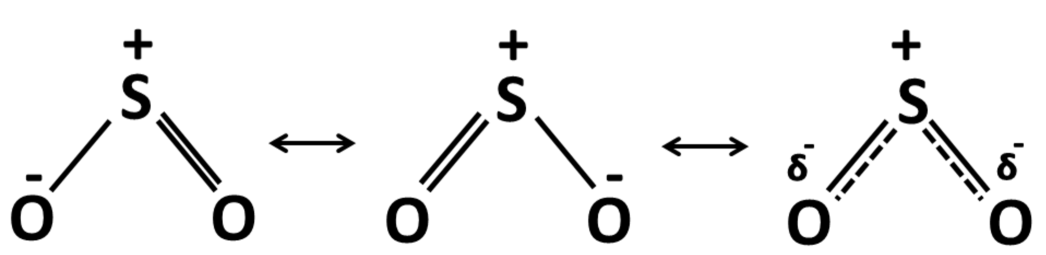
Considering the Lewis structure of SO2 molecule (Fig. 1) it can be observed that the bent structure of the molecule is such that the S-atom has a less electro-negativity while the bottom O-atoms have more of it. This makes the SO2 molecule polar. This charge difference and the distance between the charge centers produces a large permanent dipole moment. The dipole moment of SO2 is computed to be 1.7473 D while the theoretical dipole moment reported by McConkey et al. is 1.63305 D [2]. Thus the dipole moment of the neutral molecule matches satisfactorily with the earlier reported value. As a low-energy electron gets attached to the SO2 molecule forming a TNI, the charge distribution of the molecule as a whole changes and so does the dipole moment. The dipole moment of the optimized SO ground state is observed to be 1.4481 D. This 0.30 D decrease can be attributed to the attachment of the negative charge.
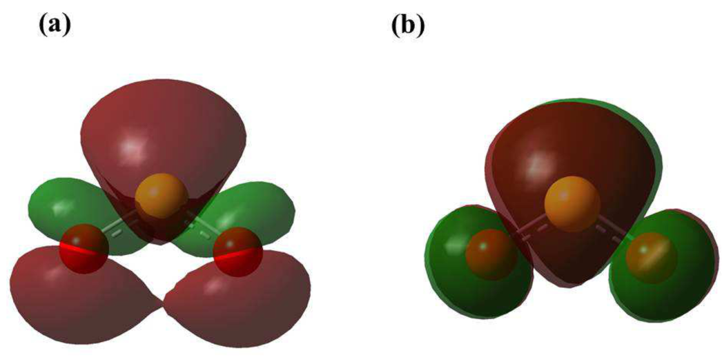
The present calculation recognizes the SO2 ground state to be an 1A1 state while the SO as a 2B1 state. This identification is in well-agreement with Gupta and Baluja [15]. The highest occupied molecular orbital (HOMO) and lowest unoccupied molecular orbital (LUMO) for these configurations are 8a1 and 9b1 respectively, for both SO2 and SO molecules, as shown in Fig. 2. The gap between the HOMO and LUMO for SO2 ground state optimized geometry is 5.12 eV while, for SO ground state optimized geometry it is 2.78 eV. The HOMO of SO rises by an amount of 9.97 eV and the LUMO of SO rises by an amount of 7.63 eV as compared to the respective HOMO and LUMO values of SO2, making the TNI SO more stable.
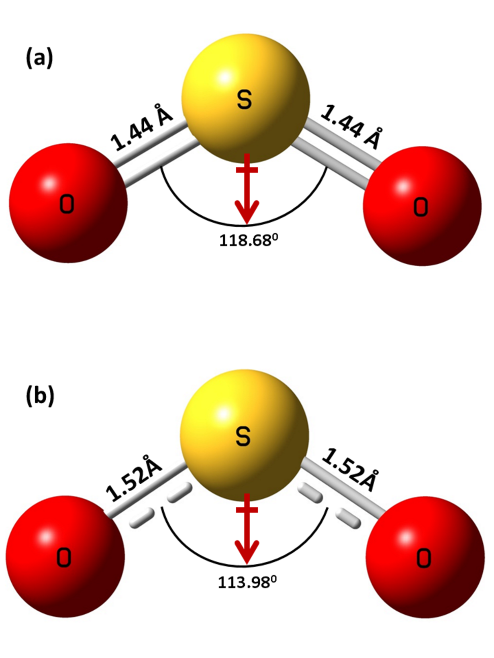
The calculated geometries of the SO2 molecule and SO negative ion are shown in Fig. 3(a) and Fig. 3(b), respectively. The neutral SO2 molecule has C2v symmetry with a S-O bond length of 1.44 and 118.680 O-S-O bond angle in the optimized state (Fig. 3(a)). After the attachment of the electron, the anion retains the C2v symmetry but the S-O bond length increases by 0.08 while the O-S-O bond angle decreases by 4.70 (Fig. 3(b)) [13]. While the direction of the dipole moment remains same in both the cases and is represented by the red arrow in Fig. 3(a) and Fig. 3(b).
3 Molecular electrostatic potential
The change in the dipole moment is associated with a change in the molecular charge distribution which can be visualized with molecular electrostatic potential (MEP) maps. When a charged particle comes in the vicinity of a molecule, the charge cloud generated through the molecule’s electrons and nuclei may serve as a guide to assess the molecule’s reactivity towards positively or negatively charged particle. Thus, the electrostatic potential maps can be used as an effective tool to accurately analyze the charge distribution of a molecule and correlate molecular properties like dipole moments, nucleophilic and electrophilic site and reactivity of the molecule towards charged reactants [25].
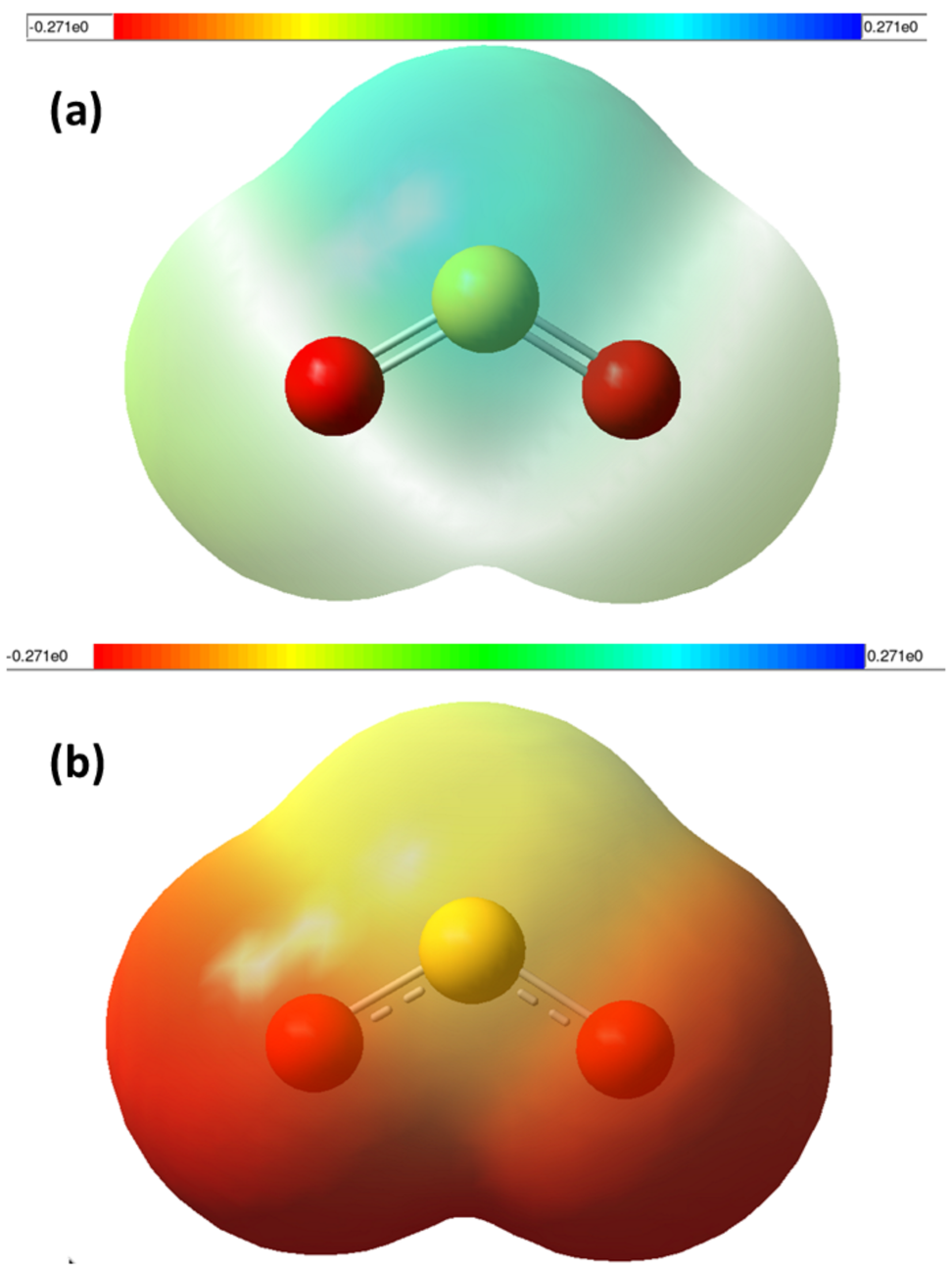
The optimized structural parameters are used to plot the MEP for SO2 and SO ground states as shown in Fig. 4(a) and Fig. 4(b), respectively. The red in the colour spectrum denotes lowest electrostatic potential value while the blue denotes the highest. The colour spectrum ranges from -0.271 a.u. (deepest red) to +0.271 a.u. (deepest blue) in both the figures (Fig. 4(a) and Fig. 4(b)). It can be observed from Fig. 4(a) that the region of lowest electrostatic potential energy, characterized by abundance of electrons, occurs near the bottom O-atoms which is in accordance with the Lewis structure (Fig. 1) and also in well agreement with the MEP reported by Esrafili and Vakili [7]. From Fig. 4(b) it can be observed that after the attachment of the low-energy electron with the SO2 molecule, the MEP map of SO shifts towards higher electron density. But the region of lowest electrostatic potential still remains near the O-atoms. This points to the fact that although the electron gets attracted towards the electro-positive S-atom, it quickly gets transfered to the O-atoms. The TNI retains the C2v symmetry like its neutral ground state and the dipole moment vector can be identified to be pointing downwards in both the cases (Fig. 3(a) and Fig. 3(b)).
The bonding features between the incoming electron and the neutral SO2 molecule can be investigated and the MEP can be quantified with the help of natural bond orbitals (NBO) analysis. The NBO 3.0 analysis, inbuilt within Gaussian 09 program package, has been carried out to observe the stabilization energies for donor-to-acceptor interactions. The NBO calculations for the SO2 ground state show that the top S-atom (labeled S(1) in Fig. 5(a)) contains a single lone pair of electrons with an occupancy of 1.993. While the two bottom O-atoms (labeled O(2) and O(3) in Fig. 5(a), respectively) share three and two lone electron pairs each thus having a more electro-negativity as compared to the S-atom. The O-atom having three lone electron pairs (O(2)) is observed with occupancies of 1.994, 1.843 and 1.545, respectively. Whereas, the other O-atom with two lone electron pairs (O(3)) has occupancies of 1.994 and 1.843 for the first and second lone pairs, respectively. Second order perturbation energy calculated for the lone pair of O(2) and bond orbital of S(1)-O(3) () interaction is 23.68 kcal/mol (Fig. 5(a)). Since the electrons form the molecular backbone, these electrons are tightly bound. The second order perturbation correction suggests that the interaction energy between the lone pair of O(2) and bond orbital of S(1)-O(3) is 76.84 kcal/mol which is more than the interaction. Thus the interaction is energetically favorable.
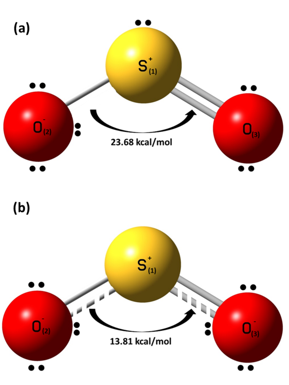
As a low-energy electron gets attached to the neutral molecule forming the TNI SO, the charge distribution of the molecule completely changes as predicted by the NBO calculations. NBO calculations for the SO ground state show that the top S(1)-atom contains a single lone pair of electrons with an occupancy of 1.998. While the two bottom O(2) and O(3) atoms share three lone electron pairs each thus having a more electro-negativity as compared to the S(1)-atom (Fig. 5(b)). The O(2) and O(3) atoms each have occupancies of 1.995, 1.983 and 1.851 for the three lone pairs, respectively. Second order perturbation energy calculated for the interaction of second lone pair of O(2) and bond orbital of S(1)-O(3) is 13.81 kcal/mol because there is no orbital for SO ground state (Fig. 5(b)). The second order perturbation energy difference of 9.87 kcal/mol (23.68 - 13.81 kcal/mol) between the for SO2 and for SO interaction suggests that the stabilization energy for SO is much less than that for neutral SO2. Thus, due to donor-acceptor interaction, SO ground state is more stable than the SO2 ground state. This is also evident from the HOMO-LUMO gap (5.12 eV for neutral SO2 and 2.78 eV for SO).
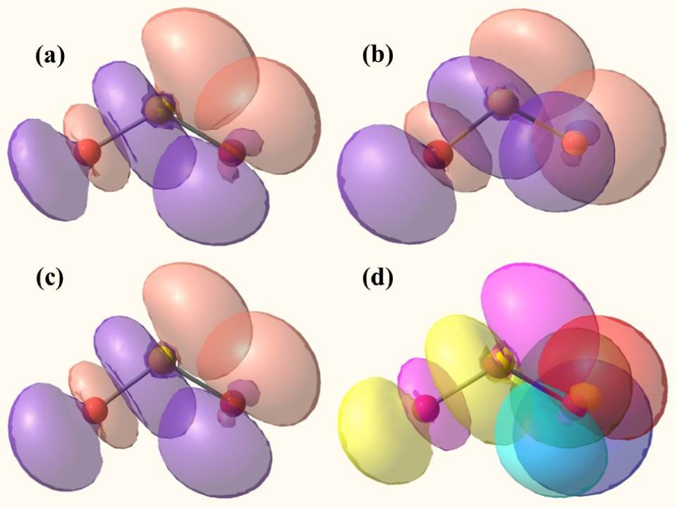
The NBO density plot for SO2 and SO has been shown in Fig. 6. Initially, for the ground state of SO2 there is significant overlap between the lone pair of O(2) and bond orbital of S(1)-O(3) (Fig. 6(a)). Since the single electron gets attached to the neutral SO2 in up-spin state ( state), the NBO density plot representing the orbital of interaction remains unchanged (Fig. 6(c)). The presence of the spin results in an extra overlap in the same LUMO orbital represented by the interaction solely due the extra electron. This can be observed from the NBO density plot for SO alpha orbital (Fig. 6(b)). The resultant NBO density plot for SO gives the orbital plot for a total sum of and orbitals (Fig. 6(d)). Comparing the resultant NBO density plot for SO to that for SO2 neutral state, it can be seen that there is a much higher overlap in the anionic state than the neutral state. This higher overlap again implies the lower interaction energy as predicted by the NBO calculations.
It can be noted from Fig. 3 that the optimized ground state configuration for the neutral SO2 (Fig. 3(a)) and TNI SO (Fig. 3(b)) are not identical. This change in the bond S-O length and O-S-O bond angle can be determined from the change in bond order using the following formula:
Bond Order=
where, and denotes number of bonding electrons and number of anti-bonding electrons, respectively.
The bond order calculated using the bonding and anti-bonding electrons from the NBO analysis (relevant to Fig. 5) are given in Table 1. As can be noted from Fig. 5(a), the resonating single S(1)-O(2) and double S(1)-O(3) bonds correspond to bond orders of 0.9 and 1.9, respectively. This means, for the optimized ground state configuration where the lone pairs of electrons redistribute themselves forming two double bonds (as in Fig. 3(a)), the bond orders will be 1.403. This result matches well with Grabowsky et al. with an error of 6.47 who reported the bond order of sulfur dioxide to be 1.5 from X-ray diffraction data [26].
For the TNI optimized ground state, the bond order comes out to be 0.47 for both the S(1)-O(2) and S(1)-O(3) double bonds. This decrease in the strength of the bond accounts for the elongation in the bond in Fig. 3(b).
4 Vibration spectral analysis
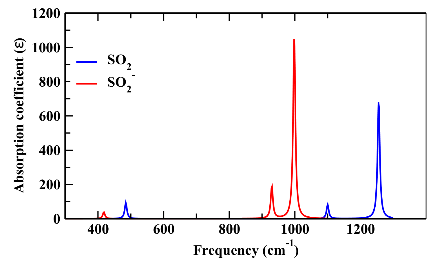
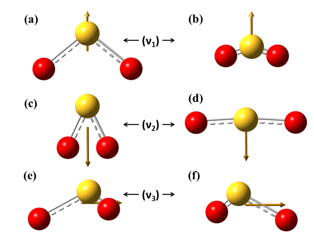
The main objective of computing the vibration spectra of the neutral SO2 and the TNI SO was to find out the vibration modes connected with the molecular structure. This in turn, helps to identify the modes responsible for the production of negative fragment ions from the TNI and also note the change in the spectra of the negatively charged molecular ion from the neutral parent molecule (Fig. 7). When the frequency of radiation matches exactly with the vibration frequency of the molecule, absorption of radiation takes place. Thus, the peaks in the IR spectra denote vibration modes at respective peak positions based on the wave number predicted theoretically by the density functional B3LYP/aug-cc-pVQZ method [6]. The analysis of the vibration spectra was done with the optimized structures of SO2 and SO. The three vibrational frequencies for neutral SO2 was computed to be 1167.96 (symmetric stretching, ), 519.22 (symmetric bending, ) and 1357.28 (asymmetric stretching, ) cm-1 respectively. While the same for SO was computed to be 979.51 (), 452.23 () and 1071.95 () cm-1 respectively, as shown in Fig. 8. The vibrational frequencies of the three normal modes of vibration for sulfur dioxide were recorded experimentally by Shelton et al. using an infrared prism-grating spectrometer [3]. The first () and third () modes both with an symmetry were observed at 1151.38 and 1361.76 cm-1, respectively. While the second mode () with a symmetry was observed at 517.69 cm-1. A. Gordon Briggs also reported the vibrational frequencies of SO2 using double-beam infrared spectrometer fitted with a diffraction grating or NaCl prism to be at 1153 (), 508 () and 1362 cm-1 () [27]. Thus the computed vibrational frequencies of the present work for SO2 matches excellently with literature [3, 27]. But no experimental or theoretical data detailing the vibrational frequencies for SO has been reported till now. The frequencies for the three modes for SO are much less as compared to the frequencies for the three modes for SO2. The change in peak positions for the two before said structures corresponding to different vibration modes are shown in Table 2.
As can be inferred from Fig. 8, the simultaneous presence of the symmetric stretching and bending modes will give rise to S- fragment formation. As the stretching may produce S-, it has to be followed by the bending mode such that the O-atoms can come close enough to form O2. The same may also produce O. The two pathways can be written as:
| (2) |
The electron affinity of O and S- being EA(O2)=0.451 eV and EA(S)=2.077 eV, cross-section of S- fragment production is much higher than O [15]. Whereas, the antisymmetric stretching mode may result in the formation of O- and SO- negative ions give by the following equations:
| (3) |
The electron affinity of O- and SO- being EA(O)=1.462 eV and EA(SO)=1.125 eV, cross-section of O- fragment production is slightly higher than SO- but both are observed [15]. This observation is in good agreement with that reported by Gope et al. [14].
5 Potential energy curves and charge distribution analysis
The potential energy plots with positive adiabatic electron affinity for SO2 and SO ground states have been shown in Fig. 9 and Fig. 10 for the following dissociation pathways:
| (4) |
| (5) |
where the B3LYP correlational functional has been used with the aug-cc-pVDZ basis set. To explore the potential energy curves for SO2 and SO optimized ground state geometries for the two dissociation pathways given by Eqns. 4 and 5, we investigated the transition states and scanned over the bond distances keeping the transition states of SO2 and SO as the initial geometry in two different ways. In the first calculation, the two O-atoms are brought closer from its equilibrium value (denoted by r0 in Fig. 9) and the energy is scanned. This results in the formation of O2 and S fragments from SO2 while, S- and O2 fragments from SO. The resulting potential energy curves for SO2 and SO optimized ground state geometries are shown in Fig. 9.
In the second case, keeping one S-O bond and O-S-O angle fixed, the other S-O is stretched from its equilibrium value (denoted by r0 in Fig. 10). This results in the formation of SO and O fragments from SO2 while, O- and SO fragments from SO. The resulting potential energy curves for SO2 and SO optimized ground state geometries are shown in Fig. 10.
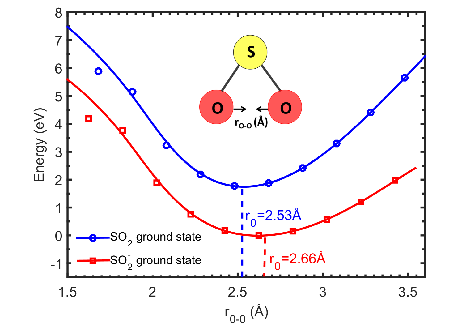
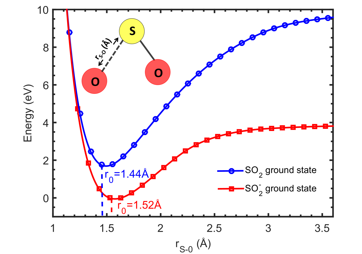
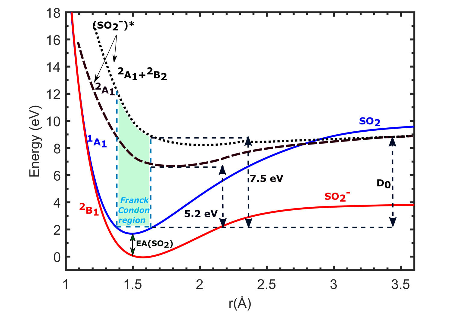
The DFT calculations predict the potential energy curves of optimized ground state of SO to be at a lower energy than its neutral parent SO2, signifying the positive electron affinity of SO2. But no SO can be observed experimentally to form at around -1.4 eV. This can be understood with the following explanations. As can be noticed from the potential energy curves in Fig. 9 and Fig. 10, there is no crossing of the SO2 and SO curves in the Franck-Condon region. Thus this resonant transition of SO2 to SO is not possible. One more reason for not observing any SO formation at around -1.4 eV could be an extremely small lifetime of the SO state, as compared to the time-of-flight which is in the order of [13]. The schematic potential energy curves shown in Fig. 11 depicts the actual SO states observed experimentally forming the two resonant peaks at 5.2 and 7.5 eV, respectively [13]. While, the SO2 and SO ground state curves are computed curves for S-O bond distance variation. The energy values for vertical transition within the Franck Condon region are calculated from TDDFT calculations and match excellently well with the experimental values reported by Jana and Nandi [13]. However, one can use the equation-of-motion coupled cluster (EOMCC) method to compute the potential energy curves for excited states of the TNI, which is beyond the scope of this work.
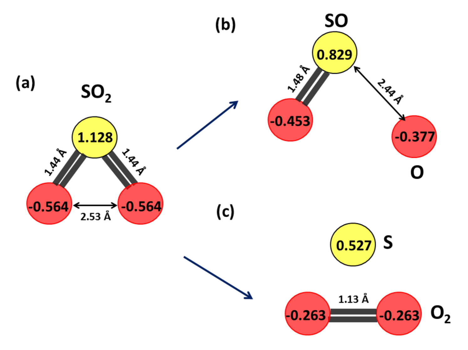
The charge distribution of neutral SO2 with equilibrium S-O and O-O bond distances of 1.44 and 2.53 respectively, is shown in Fig. 12(a), computed using Mulliken charge analysis. Mulliken charges are mathematical constructions that have no relation to physical charges. But it can be used to predict the distribution of charges within the individual atoms forming the molecule before and after dissociation. The total atomic charges add up to give the neutral SO2 molecule although, the S-atom is highly electro-positive and the O-atoms are highly electro-negative. As the S-O bond distance is slowly increased, at some value of the S-O bond coordinate the bond ruptures giving SO and O neutral fragments (Fig. 12(b)). This value of the bond was computed to be 2.44. From the Mulliken charge analysis it can be observed that both the electro-positivity of the S-atom and the electro-negativity of the O-atoms has decreased in Fig. 12(b) as compared to 12(a), predicting the neutral nature of the fragments. Similarly, with the decrease in O-O bond length, S and O2 neutral fragments can be observed to form with 1.13 O-O bond length (Fig. 12(c)).
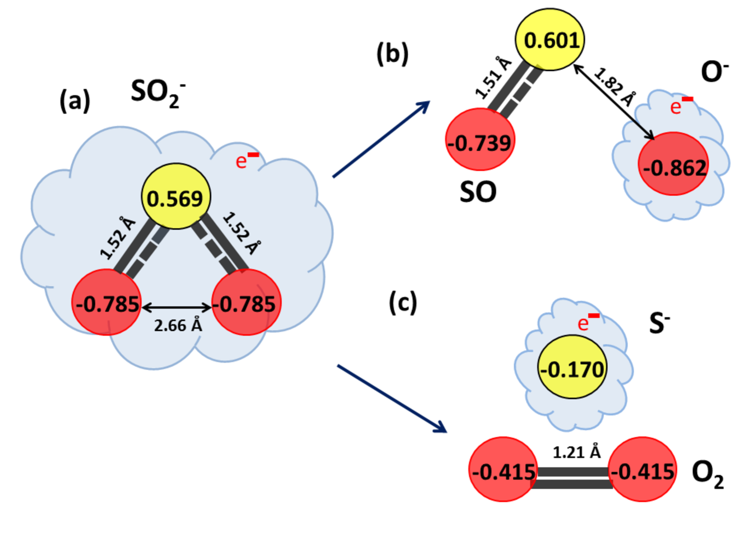
The SO anionic ground state charge distribution is shown in Fig. 13(a) with S-O and O-O equilibrium bond distances as 1.52 and 2.66 , respectively. The total charge of this anionic system can be observed to add up -1 unit of electronic charge, signifying the attached low-energy electron. As the S-O bond is gradually stretched, SO and O- fragment formation can be seen at S-O bond distance of 1.82 (Fig. 13(b)). The charge distribution predicts the SO fragment to be almost neutral, while the O- fragment carries most of the negative charge. Whereas, gradual decrease in O-O bond distance results in the formation of S- and O2 fragments, with O-O bond length being 1.21 (Fig. 13(c)) which matches excellently with the 1.21 bond length of molecular oxygen.
6 Symmetry states of the TNI
In order to get an idea about the symmetry states favorable for DEA to SO2 molecule, the optimized geometries were then used to carry out time-dependent density functional theory (TD-DFT) calculations and get the vertical energy values and symmetries of corresponding excited states for the SO molecule lying within the Franck Condon region. Then the symmetry states lying near the resonant peaks (first resonance observed in the range 4.6 - 5.6 eV and second resonance observed in the range 7.0 - 7.6 eV by different groups [1, 8, 13]) and having symmetries with considerable value of oscillator strength (f) are noted (Fig. 11). To check the validity of the calculations, the symmetries are then compared with reported experimental and theoretical data.
In TDDFT calculations, oscillator strength (f) denotes the probability of transition between energy levels in an atom or molecule with the help of absorption or emission of electromagnetic radiation. Thus a high oscillator strength for a specific transition would mean that particular transition is more probable than the others. The table showing the symmetry states for the two resonances with considerable f-value are shown in Table 3 in order of descending f-value.
| Resonance | Energy | Symmetry | Oscillator | Ref[13] |
|---|---|---|---|---|
| range (eV) | of TNI | strength (f) | ||
| First | 4.5 - 5.8 eV | A1 | 0.0515 | A1 |
| Peak | B1 | 0.0110 | ||
| Second | 7.0 - 7.6 eV | A1 | 0.0516 | |
| Peak | B2 | 0.0445 | A1 + B2 | |
| B2 | 0.0383 | |||
| B2 | 0.0319 | |||
| A1 | 0.0240 | |||
| B2 | 0.0111 |
As can be noted from the Table 3, in the energy range 4.6 - 5.6 eV, the state having the highest oscillator strength is an A1 state with f = 0.0515. Another B1 state can also be observed in the considered energy range but with very low oscillator strength and hence can be neglected. No other symmetry states were found in this energy range with considerable f-value (almost 7.2 times less than 0.05). Thus the computation predicts that the first resonant peak due to DEA to SO2 results from an A1 negative ion resonant state. This matches excellently with previous reports [1, 8, 13].
For the second resonance, negative ion resonant states lying in the energy range 7.0 - 7.6 eV with considerable f - value can be assumed to have a contribution. Six symmetry states can be observed with high f-values and are reported in Table 3. Amongst these, four are B2 and two are A1 symmetry states. From this observation, it can be concluded that the second resonance occurs due to an A1 to A1 + B2 transition. This result matches excellently with the recent experimental work on DEA to SO2 by Jana and Nandi [13]. For all the basis sets used, the oscillator strengths of A2 negative ion states are always 0. This supports the fact that if the initial state of the neutral is an A1, then A1 to A2 transition is always forbidden [1].
7 Conclusion
The theoretical and computational approach helps to visualize the attachment of a single low-energy ( 15 eV) electron to the neutral SO2 molecule thus forming the molecular anion SO. The molecular sites acting as positive centers to the incoming electron could be identified using the MEP of the neutral molecule and the results are in well agreement with the MEP reported by Esrafili and Vakili [7]. The MEP of the TNI also helped to identify the distribution of negative charge in the molecule after the attachment of the electron. Dissociation of the TNI into neutral and charged fragments based on the different vibrational modes have been explained. Computing of the potential energy curves for the dissociation pathways given in Eqn.4 and Eqn.5 have been performed for the first time for both the neutral and parent anionic ground states of SO2 molecule. The negative ion resonant states responsible for the two resonant peaks have also been identified with the help of TD-DFT calculations to the optimized ground state geometries as A1 for the first resonance and A1+B2 for the second resonance, respectively. The results match excellently with that reported experimentally from DEA to SO2 by Jana and Nandi [13].
8 Acknowledgments
We gratefully acknowledge financial supports from Science and Engineering Research Board (SERB) for supporting this research under the Project EMR/2014/000457 and for computational facility under the Project SB/FTP/CS-164/2013.
References
References
- [1] Krishnakumar E, Kumar S V K, Rangwala S A and Mitra S K 1996 J. Phys. B 29 L657
- [2] McConkey J, Malone C, Johnson P, Winstead C, McKoy V and Kanik I 2008 Phys. Rep. 466 1–103
- [3] Shelton R D, Nielsen A H and Fletcher W H 1953 J. Chem. Phys. 21 2178–2183
- [4] Maybury R H, Gordon S and Katz J J 1955 The Journal of Chemical Physics 23 1277–1281 (Preprint https://doi.org/10.1063/1.1742257)
- [5] Zhu B, Lang Z L, Ma N N, Yan L K and Su Z M 2014 Phys. Chem. Chem. Phys. 16 18017–18022
- [6] Boopathi M, Udhayakala P, Rajendiran T and Gunasekaran S 2016 J. Appl. Spectrosc. 83 12–19
- [7] Esrafili M D and Vakili M 2014 J Mol Model 20 2291
- [8] Krishnakumar E, Kumar S V K, Rangwala S A and Mitra S K 1997 Phys. Rev. A 56(3) 1945–1953
- [9] Orient O J and Srivastava S K 1983 J. Chem. Phys. 78 2949–2952
- [10] Rallis D A and Goodings J M 1971 Can. J. Chem. 49 1571–1574
- [11] Spyrou S M, Sauers I and Christophorou L G 1986 J. Chem. Phys. 84 239–243
- [12] Cadez I M, Pejcev V M and Kurepa M V 1983 J. Phys. D: Appl. Phys. 16 305–314
- [13] Jana I and Nandi D 2018 Phys. Rev. A 97(4) 042706
- [14] Gope K, Prabhudesai V S, Mason N J and Krishnakumar E 2017 J. Chem. Phys. 147 054304
- [15] Gupta M and Baluja K 2006 Phys. Rev. A 73 042702
- [16] Frisch M J, Trucks G W, Schlegel H B, Scuseria G E, Robb M A, Cheeseman J R, Scalmani G, Barone V, Mennucci B, Petersson G A, Nakatsuji H, Caricato M, Li X, Hratchian H P, Izmaylov A F, Bloino J, Zheng G, Sonnenberg J L, Hada M, Ehara M, Toyota K, Fukuda R, Hasegawa J, Ishida M, Nakajima T, Honda Y, Kitao O, Nakai H, Vreven T, Montgomery J A, Jr J E P, Ogliaro F, Bearpark M, Heyd J J, Brothers E, Kudin K N, Staroverov V N, Kobayashi R, Normand J, Raghavachari K, Rendell A, Burant J C, Iyengar S S, Tomasi J, Cossi M, Rega N, Millam J M, Klene M, Knox J E, Cross J B, Bakken V, Adamo C, Jaramillo J, Gomperts R, Stratmann R E, Yazyev O, Austin A J, Cammi R, Pomelli C, Ochterski J W, Martin R L, Morokuma K, Zakrzewski V G, Voth G A, Salvador P, Dannenberg J J, Dapprich S, Daniels A D, Farkas O, Foresman J B, Ortiz J V, Cioslowski J and Fox D J 2009 Gaussian 09, Revision D.01 (Wallingford CT: Gaussian, Inc.)
- [17] Naskar S and Das M 2017 ACS Omega 2 1795–1803
- [18] Becke A D 1988 J. Chem. Phys. 88 1053–1062
- [19] Lee C, Yang W and Parr R G 1988 Phys. Rev. B 37(2) 785–789
- [20] Becke A D 1988 Phys Rev A 38 3098
- [21] Lee C, Yang W and Parr R G 1988 Phys Rev B 37 785
- [22] Kendall R A, Dunning Jr T H and Harrison R J 1992 J. Chem. Phys. 96 6796–6806
- [23] Rösch N and Trickey S B 1997 J. Chem. Phys. 106 8940–8941
- [24] Grabowski J J, Doren J M V, DePuy C H and Bierbaum V M 1984 The Journal of Chemical Physics 80 575–577 (Preprint https://doi.org/10.1063/1.446412)
- [25] Murray J S and Sen K 1996 Molecular electrostatic potentials: concepts and applications vol 3 (Elsevier)
- [26] Grabowsky S, Luger P, Buschmann J, Schneider T, Schirmeister T, Sobolev A N and Jayatilaka D Angewandte Chemie International Edition 51 6776–6779
- [27] Briggs A G 1970 J. Chem. Educ. 47 391