Distinct charge and spin recovery dynamics in a photo-excited Mott insulator
Abstract
Pump-probe response of the spin-orbit coupled Mott insulator Sr2IrO4 reveals a rapid creation of low energy optical weight and suppression of three dimensional magnetic order on laser pumping. Post pump there is a quick reduction of the optical weight but a very slow recovery of the magnetic order - the difference is attributed to weak inter-layer exchange in Sr2IrO4 delaying the recovery of three dimensional magnetic order. We suggest that the effect has a very different and more fundamental origin. Combining spatio-temporal mean field dynamics and Langevin dynamics on the photoexcited Mott-Hubbard insulator we show that the timescale difference is not a dimensional effect but is intrinsic to charge dynamics versus order reconstruction in a correlated system. In two dimensions itself we obtain a short, almost pump fluence independent, timescale for charge dynamics while recovery time of magnetic order involves domain growth and increases rapidly with fluence. Apart from addressing the iridate Mott problem our approach can be used to analyse phase competition and spatial ordering in superconductors and charge ordered systems out of equilibrium.
pacs:
75.47.LxWith the discovery of high temperature superconductivity in the doped cuprates their parent Mott insulating state, for example La2CuO4 [1], has been extensively studied [2]. The Mott state arises due to strong local repulsion in atomic orbitals, which prevents simultaneous occupancy of both spin states, leading to an insulator at half-filling [3, 4, 5]. The localised electrons have an inter-site exchange interaction that promotes antiferromagnetic order in non frustrated lattices.
When the Mott insulator is excited by a laser pulse with appropriately chosen frequency the added energy has an impact on both the charge dynamics and the magnetic order [6, 7, 8, 9, 10, 11, 12, 13, 14, 15, 16, 17, 18, 19, 20, 21]. The pump can excite electrons from the lower Hubbard band (LHB) to the upper Hubbard band (UHB), which in real space means creation of double occupancy [22, 23, 24]. The effect is twofold: (i) the electrons excited to the UHB, and the ‘holes’ in the LHB, act as mobile carriers, leading to metallic response in the optical conductivity, and (ii) the double occupancy suppresses the magnetic moments, destroys their spatial correlation, and leads to suppression of magnetic long range order. In effect, despite being at half filling, one obtains a transient metallic state coexisting with (small) local moments, which evolves back towards its reference antiferromagnetic Mott state. It is in this context that Sr2IrO4 has thrown up several puzzles about charge and spin dynamics out of equilibrium.
A photo-excited state was realised in Sr2IrO4, a structural analog of La2CuO4. At equilibrium Sr2IrO4 is a spin-orbit coupled layered antiferromagnetic Mott insulator (AFMI) with an interaction split band [25, 26, 27, 28]. The AF is K. Laser pumping leads to dramatic changes in its magnetic and electronic properties. The two most significant observations in our reading are: (i) The rapid loss of 3D magnetic order and gain in reflectivity in response to a pump - and then a quick suppression of the reflectivity, within 1-2 picoseconds (ps) but very slow recovery of order (touching 1000 ps) [29]. This is the ‘two timescale’ issue. (ii) The persistence of low energy spectral weight in the optical conductivity even after a seeming steady state is quickly reached, suggesting a population of excited high energy electrons - the holon-doublon (HD) plasma - at long times [30]. The time dependence of planar magnetic fluctuations [29], oddly, reflects both short and long timescales! In the current interpretation [29] the in plane magnetic order and electron physics in the Mott insulator both recover quickly and the 3D recovery is delayed due to weak interlayer coupling.
We suggest that the fascinating data revealed by the experiments has another - very different - explanation. This has remained out of reach because theories of nonequilibrium phenomena need to consider the excited electronic population and also the spatial dynamics, e.g, domain growth effects, on large spatial scales. Current tools, e.g, exact diagonalisation [31, 32], dynamical mean field theory (DMFT) [33, 34, 35, 36, 37, 38]. and density matrix renormalisation group [39, 40], are either size limited or unable to access the timescale needed.
To capture the electron correlation non perturbatively and access spatio-temporal dynamics we write an equation of motion for the one body density operator in the half-filled square lattice Hubbard model and close the hierarchy by factorising the resulting four operator terms in the magnetic channel. This is ‘mean field dynamics’ (MFD) although it is in terms of the matrix rather than a local object like magnetisation. This allows access to size and time upto , where is the in-plane hopping. We also construct, benchmark, and use a Langevin dynamics (LD) scheme that allows access to lattices and time upto . We set meV ( femtoseconds) and as noted [25] for Sr2IrO4. Our results, based on a combination of MFD and LD, are the following.
(i) The pump induced suppression of order and enhancement of optical weight occurs over ps. Post pump, the optical weight reduces to reach its long time asymptote over ps, while magnetic order recovery time ranges from a few ps to ps depending on fluence.
(ii) The ‘time resolved’ magnetic fluctuation spectrum has a recovery time that varies widely, when is far from the ordering vector , and when .
(iii) While ‘charge recovery’ to a steady state value, seen in , is quick, a significant UHB electron population survives to long time, sustaining low frequency optical weight. and the weight correlates with measurements [30].
(iv) Studying a layered symmetric model with we found that the 3D ‘recovery time’ differs from the 2D value by only a factor . Key dynamical features of the layered material are two dimensional.
Model: Although Sr2IrO4 is a three dimensional multiband system with spin-orbit coupling the essential physics is in the IrO planes, controlled by a single spin-orbit coupled orbital per site subject to a Hubbard interaction. The single band model takes the conventional form: . We set the lattice spacing to 1.
We introduce the pump via a pulse of amplitude , frequency THz and pulse width fs by Peierls coupling. would be proportional to the fluence. The evolution of involves solution of the MFD dynamical equations [41], where is the number of sites. The form of this equation, its derivation, and its implementation is discussed in Supplement A [42], and primary indicators shown in Supplement B. The local magnetisation can be calculated as , where are the Pauli matrices.
While MFD reveals key features of ‘suppression-recovery’ dynamics in response to the pump, it has limitations in terms of accessible size and time that prevent study of the timescale separation observed in experiments. Electronic properties, like the upper Hubbard band occupancy, stabilize to a pump-dependent constant value on a short timescale ps, as confirmed within MFD to . Beyond a few ps, the population of electrons excited to the upper Hubbard band stabilizes to a finite time-independent value, akin to having a steady finite ’electronic temperature’ at long times. This constancy is then used in Langevin calculations on large lattices for times up to . The detailed characterization of is provided in Supplement B, where serves as a crucial input for modeling magnetic dynamics below.
To address the magnetic dynamics with high spatial resolution and long times we write a Langevin equation directly for the . In such an equation the are subject to a torque arising from the electrons, a damping, and a ‘thermal’ noise at the bath temperature . The pump excited electrons follow a Fermi distribution with temperature inferred from MFD. The equation takes the form:
| (1) | |||||
is the free energy of electrons at a temperature in the spin background , is a dissipation constant extracted from MFD, and is thermal noise with and satisfying the fluctuation-dissipation theorem at temperature . The free energy arises from the Hubbard model, , written in the spin-fermion language:
| (3) | |||||
| (5) | |||||
is the electron spin operator. in the last line are the single particle eigenvalues for the electron system in a spin background , and .
Calculating , which is , requires knowledge of the eigenvalues and eigenfunctions of the whole system. At we can calculate accurately by constructing a cluster around the site and diagonalising the cluster Hamiltonian instead of having to diagonalise the full . We use a 13 site cluster centred on , including 4 nearest neighbour sites and 8 next nearest neighbour sites. We have benchmarked this against the full diagonalisation based calculation.
The electron temperature profile obtained from MFD can be approximated as: . We find ps and and a ratio allows us to model all using only one value (see Supplement C). This leave as the only fluence dependent parameter in the Langevin equation. The fit is shown in the Supplement, where we also estimate . We set bath temperature K, the temperature for experiments were K. We use the Euler-Maruyama algorithm to solve the LD equation with step size . We average the Langevin data over 5-10 runs when extracting timescales for the magnetic response.
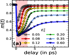
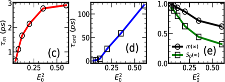
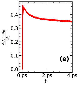
Timescales: In Fig.1 we show the time dependence of the system averaged magnetic moment and the 2D structure factor at . We set the pre-pulse values of and to 1. As the pulse hits the system both and are suppressed on a timescale ps. Post pulse, the mean moment rises quickly (panel (a)) while (panel (b)) has a strongly fluence dependent recovery time. The time axis in panel (b) is logarithmic, highlighting the wide range of recovery times. We fit the suppression-recovery dynamics in and to simple exponentials of the form: For both and we find ps. Panel (c) shows the recovery time of , while panel (d) shows the recovery time for . ranges from ps while ranges from ps. Size dependence of is shown in Supplement D.
The associated long term amplitudes and are shown in panel (e). For an experimental system in a thermal environment, and should return to their pre-pump value after the post pump system attains equilibrium. Within our MFD this does not happen since a fraction of the pump created double occupancy persists at long time. Their deexcitation requires multimagnon emission processes which have a long timescale and are beyond MFD. Even in the experiments some indicators do not return to pre-pump values over experimental observation time.
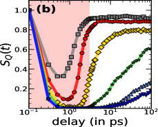
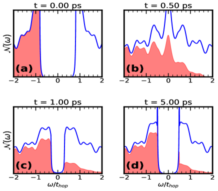
Optical response: The most dramatic effect, and readily measurable consequence, of the excited electron population is in the optical conductivity . At equilibrium the Mott insulator at low temperature should have no weight in the real part of , for , the equilibrium gap. Since the electronic timescale is ten times shorter than magnetic timescale (as inferred from the magnetic bandwidth in Fig.3, later), we calculate using the instantaneous electronic eigenstates and eigenvalues at time (see Supplement E).
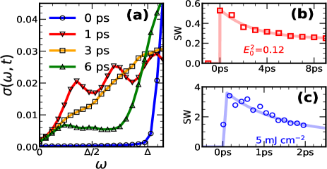
Fig.2 shows features of at , the fluence at which first drops to zero, Fig.1.(b). In Fig.2(a) at shows the absence of any weight for . Between and ps the weight in the interval rises quickly, reaching a maximum around 1ps and declining thereafter. deviates from a Drude response due to the suppressed low energy density of states and the strong orientational disorder in the magnetic background.
In panel (b) we show the integrated weight over a small window , as had been done in the pump probe experiment [30]. The two noteworthy features are (i) the quick decay to a long time value with a time constant ps, (ii) a ‘long time’ value that is of the peak. Panel (c) shows the time dependence of the weight extracted from the experimental data in Fig.2(g) in [30].
It is not coincidental that the optical timescale and the moment recovery time are comparable. Both arise from the deexcitation of electrons pushed to the upper band by the pump pulse. The deexcitation reduces double occupancy, trying to restore the moment magnitude, and the reducing number of electrons in the UHB, and ‘holes’ in the LHB, reduces the low energy optical weight. Broadly speaking, these process are related to the quick - local - charge relaxation in the system, operative on a few ps timescale. This contrasts with the long timescale for restoring global order. We next look at an indicator - already probed experimentally - of the momentum and ‘time resolved’ magnetic fluctuation spectrum.
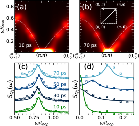
Spin dynamics: Experiments have measured the 2D dynamical structure factor of the spins via time resolved resonant inelastic X-ray scattering (tr-RIXS) [29]. In contrast to the equilibrium case this collects ‘’ data of magnetic fluctuations over a time interval around a reference time . The background state is time evolving so the resulting depends on the reference time . We compute the corresponding object based on LD data: We set ps and used ps.
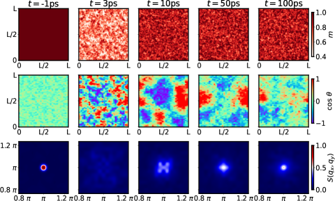
Fig.3(a)-(b) show as colour maps for two values of reference time, ps and ps. On the axis is , on the axis is , and the intensity is coded in colour. The results are at , a ‘strong fluence’ case where magnetic order recovers very slowly. Superposed on (a) and (b) is the equilibrium spin wave dispersion of the AF state. At both the spectrum far from the ordering wavevector looks similar to except for a correction due to moment size. However near the spectral weight distribution is very different from : at ps the difference is drastic while at ps still has not recovered its character. Note that these times are much greater than or that we have discussed.
To highlight the dependence of the recovery process panels (c) and (d) show the lineshapes for two momenta: one situated far from at , the other near at , In each of these we have highlighted by an arrow. It is obvious that for the peak location in has stabilised within ps. At however the peak location is far from stabilised even at ps. This is not surprising given that the ordering timescale at this fluence is ps, Fig.1(d), and it would take for the spectrum near to stabilise.
More generally, the results in Fig.3 suggest that the ‘recovery’ time for the magnetic fluctuation spectrum is strongly dependent, and this timescale ranges from when is far from to when . The RIXS spectrum probes moment size recovery and short range correlations when far from , and progressively longer range correlation of the moments when . In the next figure we wish to show the ‘domain growth’ physics that underlies this phenomena.
Spatial behaviour: Fig.4 shows the detailed spatial behaviour of the moment size in the top row, differently oriented AF domains (coded by colour) in the middle row, and the instantaneous structure factor , in the bottom row, for time ranging from ps to ps. This is a strong pulse situation, the same as studied for .
As the pulse hits the system the mean magnetic moment reduces to 40 of its original value and then quickly recovers to a stable value by 10ps. There is no spatial structure to the fluctuations in . The middle row shows the pre-pulse perfect order at ps - a single AF domain. At ps, where the moment value is still suppressed, there is a patchwork of small domains with linear dimension of a few lattice spacings (the map is ). By ps the moments have stabilised and there are only a few large competing domains. ps and ps show the increasing dominance of one (green-blue) domain. The lowest row shows the dependence of near the ordering wavevector. The perfect order in the pre-pulse state is destroyed at 3ps due to suppression of the moments. Then there is a slow growth of intensity near and a clear peak becomes visible only at ps.
In the domain pictures we have gauged out the oscillation of Neel order and plotted equivalent ‘ferromagnetic’ domains with net moment pointing in different directions. If a domain has linear dimension , probing it should lead to a fluctuation spectrum mimicking the bulk order as long as . The typical for us is time dependent, so the moderate size domains at ps well capture the fluctuation at , while we would need ps to capture fluctuations near .
We discuss two issues now that have bearing on the theory-experiment comparison and the reliability of the calculation itself. (i) 2D versus 3D: The experimental paper [29] suggested that the growth of 3D order was slow because the interplanar magnetic exchange was , the in plane value. It was implicit that recovery of 2D order was quick and the delayed 3D recovery was a effect. We have shown that 2D recovery itself is inevitably delayed. Does that mean an even more delayed 3D recovery? We did dynamics on a ‘layered’ Heisenberg model (Supplement F) with down to . Naively one may have expected . We find the ratio to be 2! This is because 2D is the lower critical dimension for models and any small is a singular perturbation [43, 44]. (ii) Thermalisation: Within the MFD framework, from which we extract our , there are pump induced holon-doublon excitations which persist to long time, and their effective temperature differs from the apparent temperature sensed by the magnetic moments. For a system that equilibriates, these two temperatures should finally be the same. The electronic excitation scale the magnetic excitation scale, so multimagnon emission processes are needed to deexcite electrons. The timescale arising from such processes has been estimated to be , [45] where . Plugging in meV and meV, we would get a decay time ps, which is than the experimental observation time or our run time.
Conclusion:
Pump-probe experiments have made it possible to
temporarily ‘metallise’ an antiferromagnetic Mott insulator
and suppress it’s magnetic order by creating double occupancy
and destroying the magnetic moment. The key question was how
this strongly perturbed state evolves back towards the
reference AFMI at long times.
With the experimental data on Sr2IrO4 setting a
reference we
set up a hierarchical scheme that addresses this
nonequilibrium correlated problem on large spatial scales
in real time. We conclude that
the ‘charge physics’, of optics etc, is dominantly local,
quick, and mostly insensitive to fluence. The magnetic
order recovery, however, is strongly non local,
involves growth of domains, and brings in a fluence and
system size dependent timescale.
Momentum resolved magnetic excitations probe different
spatial scales, and hence different recovery times.
While our specific results are on the AFMI in Sr2IrO4,
the mean field dynamics framework, and it’s reduced
Langevin counterpart, can be readily adapted to address
large spatial scale nonequilibrium phenomena in
ordered systems like superconductors or charge density waves.
We acknowledge use of the HPC clusters at HRI. PM thanks Rajdeep
Sensarma for a discussion.
References
- [1] P. M. Grant, S. S. P. Parkin, V. Y. Lee, E. M. Engler, M. L. Ramirez, J. E. Vazquez, G. Lim, R. D. Jacowitz, and R. L. Greene, Evidence for superconductivity in La2CuO4, Phys. Rev. Lett. 58, 2482 (1987).
- [2] Patrick A. Lee, Naoto Nagaosa, and Xiao-Gang Wen, Doping a Mott insulator: Physics of high-temperature superconductivity, Rev. Mod. Phys. 78, 17 (2006).
- [3] Masatoshi Imada, Atsushi Fujimori, and Yoshinori Tokura, Metal-insulator transitions Rev. Mod. Phys. 70, 1039 – 1998.
- [4] J. P. Perdew and Alex Zunger, Self-interaction correction to density-functional approximations for many-electron systems, Phys. Rev. B 23, 5048 – 1981.
- [5] Vladimir I. Anisimov, Jan Zaanen, and Ole K. Andersen, Band theory and Mott insulators: Hubbard U instead of Stoner I Phys. Rev. B 44, 943 – 1991.
- [6] Alberto de la Torre, Dante M. Kennes, Martin Claassen, Simon Gerber, James W. McIver, and Michael A. Sentef, Colloquium: Nonthermal pathways to ultrafast control in quantum materials, Rev. Mod. Phys. 93, 041002 – 2021
- [7] Yuta Murakami, Denis Golež, Martin Eckstein, Philipp Werner, Photo-induced nonequilibrium states in Mott insulators, arXiv:2310.05201 [cond-mat.str-el]
- [8] Hideo Aoki, Naoto Tsuji, Martin Eckstein, Marcus Kollar, Takashi Oka, and Philipp Werner, Nonequilibrium dynamical mean-field theory and its applications, Rev. Mod. Phys. 86, 779 – 2014
- [9] Martin Eckstein and Philipp Werner, Photoinduced States in a Mott Insulator Phys. Rev. Lett. 110, 126401 – 2013
- [10] Takashi Oka and Hideo Aoki, Photoinduced Tomonaga-Luttinger-like liquid in a Mott insulator Phys. Rev. B 78, 241104(R) – 2008
- [11] Zhuoran He and Andrew J. Millis Photoinduced phase transitions in narrow-gap Mott insulators: The case of VO2 Phys. Rev. B 93, 115126 – 2016
- [12] Takashi Oka and Hideo Aoki, Photoinduced Tomonaga-Luttinger-like liquid in a Mott insulator Phys. Rev. B 78, 241104(R) – 2008
- [13] Jiajun Li, Markus Müller, Aaram J. Kim, Andreas M. Läuchli, and Philipp Werner, Twisted chiral superconductivity in photodoped frustrated Mott insulators Phys. Rev. B 107, 205115 – 2023
- [14] M. Ligges, I. Avigo, D. Golež, H.U.R. Strand, Y. Beyazit, K. Hanff, F. Diekmann, L. Stojchevska, M. Kalläne, P. Zhou, K. Rossnagel, M. Eckstein, P. Werner, and U. Bovensiepen, Ultrafast Doublon Dynamics in Photoexcited -TaS2, Phys. Rev. Lett. 120, 166401 – 2018
- [15] Takashi Oka, Nonlinear doublon production in a Mott insulator: Landau-Dykhne method applied to an integrable model, Phys. Rev. B 86, 075148 – 2012
- [16] Ryota Ueda, Kazuhiko Kuroki, and Tatsuya Kaneko, Photoinduced -pairing correlation in the Hubbard ladder, Phys. Rev. B 109, 075122 – 2024
- [17] Julián Rincón, Elbio Dagotto, and Adrian E. Feiguin, Photoinduced Hund excitons in the breakdown of a two-orbital Mott insulator, Phys. Rev. B 97, 235104 – 2018
- [18] Jiajun Li and Martin Eckstein, Nonequilibrium steady-state theory of photodoped Mott insulators, Phys. Rev. B 103, 045133 – 2021
- [19] K. Kimura, H. Matsuzaki, S. Takaishi, M. Yamashita, and H. Okamoto, Ultrafast photoinduced transitions in charge density wave, Mott insulator, and metallic phases of an iodine-bridged platinum compound, Phys. Rev. B 79, 075116 – Published 18 February 2009
- [20] Eckstein, M., Werner, P. Ultra-fast photo-carrier relaxation in Mott insulators with short-range spin correlations, Sci Rep 6, 21235 (2016)
- [21] Akira Takahashi, Hisashi Itoh, and Masaki Aihara, Photoinduced insulator-metal transition in one-dimensional Mott insulators, Phys. Rev. B 77, 205105 – 2008
- [22] Zala Lenarčič and Peter Prelovšek, Ultrafast Charge Recombination in a Photoexcited Mott-Hubbard Insulator, Phys. Rev. Lett. 111, 016401 – 2013.
- [23] T.-S. Huang, C. L. Baldwin, M. Hafezi, and V. Galitski, Spin-mediated Mott excitons, Phys. Rev. B 107, 075111 – 2023.
- [24] P. Wróbel and R. Eder,Excitons in Mott insulators, Phys. Rev. B 66, 035111 – 2002.
- [25] B. J. Kim et.al. Novel Mott State Induced by Relativistic Spin-Orbit Coupling in , PRL 101, 076402 (2008).
- [26] C. L. Lu, J.-M. Liu, The Jeff = 1/2 Antiferromagnet Sr2IrO4: A Golden Avenue toward New Physics and Functions. Adv. Mater. 2020, 32, 1904508 Adv. Mater. 2020, 32, 1904508.
- [27] R. Arita, J. Kuneš, A. V. Kozhevnikov, A. G. Eguiluz, and M. Imada, Ab initio Studies on the Interplay between Spin-Orbit Interaction and Coulomb Correlation in Sr2IrO4 and Ba2IrO4, Phys. Rev. Lett. 108, 086403 – 2012.
- [28] Li, Q., Cao, G., Okamoto, S. et al. Atomically resolved spectroscopic study of Sr2IrO4: Experiment and theory. Sci Rep 3, 3073 (2013).
- [29] Dean, M., Cao, Y., Liu, X. et al. Ultrafast energy- and momentum-resolved dynamics of magnetic correlations in the photo-doped Mott insulator , Nature Mater 15, 601–605 (2016).
- [30] Mehio, O., Li, X., Ning, H. et al. A Hubbard exciton fluid in a photo-doped antiferromagnetic Mott insulator. Nat. Phys. 19, 1876–1882 (2023).
- [31] Akira Takahashi, Hisashi Itoh, and Masaki Aihara, Photoinduced insulator-metal transition in one-dimensional Mott insulators, Phys. Rev. B 77, 205105 – 2008.
- [32] Satoshi Ejima, Florian Lange, and Holger Fehske, Photoinduced metallization of excitonic insulators, Phys. Rev. B 105, 245126 – 2022
- [33] Afanasiev, Gatilova, et.al. Ultrafast Spin Dynamics in Photodoped Spin-Orbit Mott Insulator Phys. Rev. X 9, 021020 (2019).
- [34] P. Werner, N. Tsuji, and M. Eckstein, Nonthermal Symmetry-Broken States in the Strongly Interacting Hubbard Model, Phys. Rev. B 86, 205101 (2012).
- [35] J. H. Mentink and M. Eckstein, Ultrafast Quenching of the Exchange Interaction in a Mott Insulator, Phys. Rev. Lett. 113, 057201 (2014).
- [36] K. Balzer, F. A. Wolf, I. P. McCulloch, P. Werner, and M. Eckstein, Nonthermal Melting of Néel Order in the Hubbard Model, Phys. Rev. X 5, 031039 (2015).
- [37] M. Eckstein and P. Werner, Ultra-fast Photo-Carrier Relaxation in Mott Insulators with Short-Range Spin Correlations, Sci. Rep. 6, 21235 (2016).
- [38] J. K. Freericks, V. M. Turkowski, and V. Zlatić, Nonequilibrium Dynamical Mean-Field Theory Phys. Rev. Lett. 97, 266408 – 2006
- [39] Satoshi Ejima, Florian Lange, and Holger Fehske, Nonequilibrium dynamics in pumped Mott insulators, Phys. Rev. Research 4, L012012 – 2022.
- [40] Satoshi Ejima, Florian Lange, and Holger Fehske, Photoinduced metallization of excitonic insulators, Phys. Rev. B 105, 245126 – 2022.
- [41] Chern, Gia-Wei and Barros, Kipton et.al. Semiclassical dynamics of spin density waves, PhysRevB.97.035120, (2018).
- [42] All sections are included in the supplementary material. In Supplement A, we derive the mean-field equation of motion for equal time correlations under an external electric pulse. In Supplement B, we establish the relationship between the electric field and effective electronic temperature. Supplement C compares the dynamics from MFD and non-equilibrium Langevin dynamics. In Supplement D, we discuss the effect of system size. Supplement E provides the formula we used to calculated the conductivity. Supplement F compares the 3D recovery dynamics to the layer-averaged 2D recovery of the structure factor in a quasi-2D Heisenberg model with .
- [43] Bang-Gui Liu, A nonlinear spin-wave theory of quasi-2D quantum Heisenberg antiferromagnets J. Phys.: Condens. Matter 4 8339 (1992)
- [44] A. Du and G. Z. Wei, Magnetic Properties of Layered Heisenberg Ferromagnets, Aust. J. Phys., 1993, 46, 571-81.
- [45] Rajdeep Sensarma, David Pekker, Ehud Altman, Eugene Demler, Niels Strohmaier, Daniel Greif, Robert Jördens, Leticia Tarruell, Henning Moritz, and Tilman Esslinger Lifetime of double occupancies in the Fermi-Hubbard model Phys. Rev. B 82, 224302 – (2010)
Supplementary to “Distinct charge and spin recovery dynamics
in a photo-excited Mott insulator”
Sankha Subhra Bakshi and Pinaki Majumdar
Harish-Chandra Research Institute
(A CI of Homi Bhabha National Institute),
Chhatnag Road, Jhusi, Allahabad 211019
I Supplement A: Mean field dynamics (MFD)
In this section we derive an equation of motion for the ‘density operator’ , from which the local magnetisation and local density can be computed. We start with a single band repulsive Hubbard model
| (7) |
Where is the nearest neighbor hopping with value . We can rewrite the interaction term in the following way:
| (8) |
Where the local density operator is , and the local spin operator is , being the Pauli matrices. is any arbitrary SO(3) unit vector. The interaction term can be rewritten as
| (9) |
where
| (10) |
Now we write the Heisenberg equation for
| (11) |
The bilinear term in produces bilinear correlations
| (12) |
The interaction term leads to:
| (13) |
We take average of both sides and write . The interaction term produces a term of the form . To close the equation we approximate . This leads to:
| (14) |
Where,
| (15) |
Modeling the pump: The electrons in the system couple with the vector potential associated with the electromagnetic field of the laser pulse. This can be included in the electronic part of the Hamiltonian via Peierl’s substitution which transforms the tight-binding hopping parameter as
| (16) |
Where and are the frequency and the width of the pulse. Equipped with these, we solve the MFD equation using the RK4 algorithm. The direction of the field is kept at to the x-axis.
II Supplement B: Electronic temperature from MFD
We focus on the mean-field dynamics on a lattice with a pulse width of . We maintain the pump frequency approximately equal to the gap in the density of states and vary only the amplitude . We calculate the instantaneous occupation function :
| (17) |
Here, are the eigenvalues in the instantaneous background at time . The operator is the -th instantaneous annihilation operator at time , which annihilates an electron in the state corresponding to in the background field. The density of states and the occupied part of the density of states are shown in Fig 1(a)-(d). In Fig.1(e) we plot the time dependence of the double occupancy, calculated from the instantaneous magnetic background. The double occupancy at half filling can be estimated from the average square of the magnetic moment size as , where the average is over all the sites.
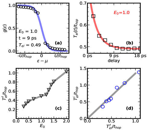
While initially has a ‘non thermal’ look it quickly takes a form that can be approximated by a Fermi distribution with electronic temperature . Fig.2 shows such a fit. We parameterize the extracted with an exponential decay:
| (18) |
where is the initial electron temperature (as soon as the pulse passes) and is the long time electron temperature. We find that is mainly fluence independent. From these we can establish a relationship between and . We find as shown in Fig.2., though the initial distribution cannot be fitted with an Fermi-distribution reliably.
III Supplement C: Benchmarking Langevin with MFD
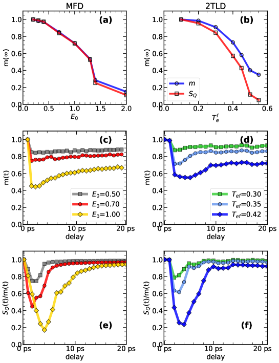
One can write a Langevin-like stochastic equation [1], where the origin of the damping is phenomenological. We adapt this formulation to calculate the effective torque arising from the excited electron population. The spins experience a lower temperature, . We call this scheme 2-Temperature Langevin Dynamics (2TLD) [Discussed in the main text]. On a lattice size of , we run 2TLD with the obtained from the MFD. We used various values of the dissipation coefficient in the LD to match LD results with MFD. If we want to single for all then seems to be a reasonable choice, however it requires a larger value of . We compare the transient dynamics from MFD and LD in Fig.3.
In Fig.3 top panels we plot the steady-state value of and as a function of obtained from both methods. In the middle panel, we plot , which shows similar quick suppression followed by a sub-10-ps recovery. In the bottom panels, we plot .
As this is a very small system, the domain dynamics is severely size-dependent at this lattice length. Nonetheless, the ratio captures only the domain recovery, ignoring the effect of recovery of on . We see that the 2TLD method is reasonable within the range we want to capture for larger system sizes compared to the MFD. We keep small, , for 2TLD.
IV Supplement D: Averaging and dependence in LD
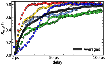
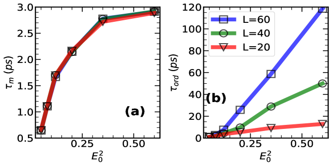
The order recovery process is highly stochastic due to the role of domain growth. Therefore, it is necessary to average the recovery over multiple thermal runs. We used 5 to 10 different runs to average . In Fig.4, we present the different traces as well as the averaged curve. Although the recovery timescale for the average magnetic moment does not significantly depend on the system size, the recovery timescale for is size-dependent, as shown in Fig.5.
V Supplement E: Optical conductivity calculation
To calculate the optical conductivity, we assume a separation of time scales between charge and spin dynamics. For an instantaneous background , we diagonalize the single particle Hamiltonian as described in the main text. This yields the eigenfunctions () and eigenvalues (). The current operator is defined as . The electron temperature is set to . The conductivity is then computed as follows:
| (19) |
where denotes the Fermi function. A more rigorous expression for conductivity, using two-time correlation, is provided in [2].
VI Supplement F: Recovery in the Heisenberg Model
At half-filling and large Hubbard model maps to the Heisenberg model.
| (20) |
where , with being the average magnetic moment (magnitude of 1 at equilibrium) and a unit vector in . In a layered system the in-plane exchange is the interlayer exchange . The spin dynamics follows the Landau–Lifshitz–Gilbert-Brown (LLGB) equation:
| (21) |
where represents thermal noise from a bath at temperature [3]. Numerical method like the Suzuki-Trotter decomposition is employed to solve this equation [4].
Initial condition: After the pump pulse passes, the system is assumed to have a reduced magnetic moment and a distorted spin configuration. The evolution parameters are , , , and .
To analyze the effect of photo-pumping on recovery dynamics, we make the following approximations:
-
•
The initial state corresponds to and is derived from a thermal state with (where is the critical temperature).
-
•
The system evolves with nearest-neighbor in-plane coupling and dissipation rate .
Parameters: We set and keep the ratio constant and small (, ). The bath temperature is maintained at , and is set to 0.05. We use a 3D lattice of dimensions (10 layers in the -direction). We compute the 2D structure factor averaged over all layers and the 3D structure factor . Starting with an initial state where all layers have , the system evolves with varying . Five parallel runs were averaged for the 3D structure factor growth.
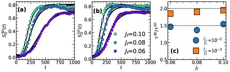
2D vs 3D recovery: Fig.6 shows the detailed dynamics. Both 2D and 3D structure factor growths are fitted with , and we extract two timescales, and , plotting their ratio with . Although the inter-layer coupling is 1000 times weaker than the in-plane coupling, the recovery timescale is only a factor of approximately 2 times larger.
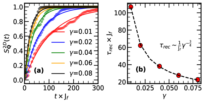
Role of dissipation: Fig.7 shows the dependence of on . With values ranging from 0.01 to 0.05. Our results indicate that .
The bibliography
[1] Pui-Wai Ma and S. L. Dudarev, Longitudinal magnetic fluctuations in Langevin spin dynamics, Phys. Rev. B 86, 054416 (2012), DOI: 10.1103/PhysRevB.86.054416
[2] Zala Lenarčič, Denis Golež, Janez Bonča, and Peter Prelovšek, Optical response of highly excited particles in a strongly correlated system, Phys. Rev. B 89, 125123 (2014), DOI: 10.1103/PhysRevB.89.125123
[3] Sauri Bhattacharyya, Sankha Subhra Bakshi, Saurabh Pradhan, and Pinaki Majumdar, Strongly anharmonic collective modes in a coupled electron-phonon-spin problem, Phys. Rev. B 101, 125130 (2020), DOI: 10.1103/PhysRevB.101.125130
[4] Pui-Wai Ma and S. L. Dudarev, Langevin spin dynamics, Phys. Rev. B 83, 134418 (2011), DOI: 10.1103/PhysRevB.83.134418