Distributed Computation Offloading for Energy Provision Minimization in WP-MEC Networks with Multiple HAPs
Abstract
This paper investigates a wireless powered mobile edge computing (WP-MEC) network with multiple hybrid access points (HAPs) in a dynamic environment, where wireless devices (WDs) harvest energy from radio frequency (RF) signals of HAPs, and then compute their computation data locally (i.e., local computing mode) or offload it to the chosen HAPs (i.e., edge computing mode). In order to pursue a green computing design, we formulate an optimization problem that minimizes the long-term energy provision of the WP-MEC network subject to the energy, computing delay and computation data demand constraints. The transmit power of HAPs, the duration of the wireless power transfer (WPT) phase, the offloading decisions of WDs, the time allocation for offloading and the CPU frequency for local computing are jointly optimized adapting to the time-varying generated computation data and wireless channels of WDs. To efficiently address the formulated non-convex mixed integer programming (MIP) problem in a distributed manner, we propose a Two-stage Multi-Agent deep reinforcement learning-based Distributed computation Offloading (TMADO) framework, which consists of a high-level agent and multiple low-level agents. The high-level agent residing in all HAPs optimizes the transmit power of HAPs and the duration of the WPT phase, while each low-level agent residing in each WD optimizes its offloading decision, time allocation for offloading and CPU frequency for local computing. Simulation results show the superiority of the proposed TMADO framework in terms of the energy provision minimization.
Index Terms:
Mobile edge computing, wireless power transfer, multi-agent deep reinforcement learning, energy provision minimization.I Introduction
The fast development of Internet of Things (IoT) has driven various new applications, such as automatic navigation and autonomous driving [1]. These new applications have imposed a great demand on the computing capabilities of wireless devices (WDs) since they have computation-intensive and latency-sensitive tasks to be executed [2]. However, most WDs in IoT have low computing capabilities. Mobile edge computing (MEC) [3] has been identified as one of the promising technologies to improve the computing capabilities of WDs, through offloading computing tasks from WDs to surrounding MEC servers acted by access points (APs) or base stations (BSs). In this way, MEC servers’ computing capabilities could be shared with WDs [4]. For MEC, there are two computation offloading policies, i.e., the binary offloading policy and the partial offloading policy [5], [6]. The former is appropriate for indivisible computing tasks, where each task is either computed locally at WDs (i.e., local computing mode) or entirely offloaded to the MEC server for computing (i.e., edge computing mode). The latter is appropriate for arbitrarily divisible computing tasks, where each task is divided into two parts. One part is computed locally at WDs, and the other part is offloaded to the MEC server for computing. Works [7] and [8] focused on the partial offloading policy in a multi-user multi-server MEC environment, formulated a non-cooperative game, and proved the existence of the Nash equilibrium.
Energy supply is a key factor impacting the computing performance, such as the computing delay and computing rate, and the offloading decisions, such as computing mode selections under the binary offloading policy and the offloading volume under the partial offloading policy. However, most WDs in IoT are powered by batteries with finite capacity. Frequent battery replacement is extremely cost or even impractical in hard-to-reach locations, which limits the lifetime of WDs. To break this limitation, wireless power transfer (WPT) technology [9, 10], which realizes wireless charging of WDs by using hybrid access points (HAPs) or energy access points (EAPs) to broadcast radio frequency (RF) signals, is widely believed as a viable solution due to its advantages of stability and controllability in energy supply [11, 12]. As such, wireless powered mobile edge computing (WP-MEC) has recently aroused increasing attention [13] since it combines the advantages of MEC and WPT technologies, i.e., enhancing computing capabilities of WDs while providing sustainable energy supply.
| Ref. | Goal | Energy supply | Multiple servers | Binary offloading | Long-term optimization | Computation data demand of network | Distributed computation offloading |
|---|---|---|---|---|---|---|---|
| [14] | computation rate | ||||||
| [15] | energy efficiency | ||||||
| [16] | energy provision | ||||||
| [18] | energy provision | ||||||
| [19] | energy provision | ||||||
| [20] | energy efficiency | ||||||
| [21] | energy efficiency | ||||||
| [22] | computation rate | ||||||
| [23] | computation delay | ||||||
| [24] | energy provision | ||||||
| Ours | energy provision | ||||||
| denotes the existence of the feature. | |||||||
Due to the coupling of the energy supply and the communication/computation demands of WDs, the critical issue in WP-MEC networks is how to reasonably allocate energy resource and make offloading decisions, so as to optimize various network performance. Consequently, many works [14, 15, 16, 17, 18, 19, 20, 21] have been done to address the issue. Under the binary offloading policy, Bi et al. [14] maximized the weighted sum computation rate of WDs in a multi-user WP-MEC network by jointly optimizing WDs’ computing mode selections and the time allocation between WPT and data offloading. Under the max-min fairness criterion, Zhou et al. [15] maximized the computation efficiency of a multi-user WP-MEC network by jointly optimizing the duration of the WPT phase, the CPU frequency, the time allocation and offloading power of WDs. While Chen et al. [16] considered a WP-MEC network where a multiple-antenna BS serves multiple WDs, and proposed an augmented two-stage deep Q-network (DQN) algorithm to minimize the average energy requirement of the network. Under the partial offloading policy, Park et al. [17] investigated a WP-MEC with the simultaneous wireless information and power transmission (SWIPT) technique, and minimized the computation delay by jointly optimizing the data offloading ratio, the data offloading power, the CPU frequency of the WD and the power splitting ratio. In a single-user WP-MEC network consisting of a multi-antenna EAP, a MEC server and a WD, Wang et al. [18] minimized the transmission energy consumption of the EAP during the WPT phase by jointly optimizing the energy allocation during the WPT phase at the EAP and the data allocation for offloading at the WD. In a two-user WP-MEC network with the nonorthogonal multiple access (NOMA) protocol, Zeng et al. [19] also minimized the transmission energy consumption of the EAP, similar to [18], under the energy and computing delay constraints, and proposed an iterative algorithm to solve it. Different from the above works, works [20] and [21] focused on the backscatter-assisted WP-MEC network, where WDs harvest energy for local computing and data offloading through active transmission and backscatter communication. Considering the limited computation capacity of the MEC server, Ye et al. [20] respectively maximized the computation energy efficiency and the total computation bits by proposing two resource allocation schemes. By leveraging the NOMA protocol to enhance backscatter communication, Du et al. [21] maximized the computation energy efficiency. The aforementioned works [14, 15, 16, 17, 18, 19, 20, 21], however, only focused on the WP-MEC networks with a single HAP, which makes it difficult to efficiently process the massive amount of the computation data offloaded from a large number of WDs.
Recently, few works [22], [23] have studied the WP-MEC networks with multiple HAPs, which are practical for large-scale IoT. Specifically, with the goal of computation rate maximization for a single time slot, Zhang et al. [22] first obtained the near-optimal offloading decisions by proposing an online deep reinforcement learning (DRL)-based algorithm, and then optimized the time allocation by designing a Lagrangian duality-based algorithm. While Wang et al. [23] focused on the long-term average task completion delay minimization problem, and proposed an online learning algorithm implemented distributively for HAPs to learn both the duration of the WPT phase and offloading decisions at each time slot. Actually, besides the computation rate [14], [22], computation efficiency [15], [20], and computation delay [17], [23], the energy provision is also a very important metric for evaluating the design of the WP-MEC networks [24]. However, as far as we know, the energy provision minimization of the WP-MEC networks with multiple HAPs has seldom been studied. Although works [16] and [18] have studied it in the WP-MEC networks with one HAP, the design in [16] and [18] can not be applied in the WP-MEC networks with multiple HAPs due to the complex association between WDs and HAPs.
To fill this gap, we study the long-term energy provision minimization problem of a multi-HAP WP-MEC network in a dynamic environment, where WDs harvest energy from the RF signals of HAPs, and then compute or offload the computation data under the binary offloading policy. Besides the energy constraint, the computing delay and computation data demand constraints should be satisfied in order to ensure the computing performance of the network. The computing delay constraint ensures that the generated computation data at each time slot is computed either locally or remotely at HAPs within the acceptable duration. The computation data demand constraint ensures that the total amount of the processed computation data at each time slot is no smaller than the required computation data demand, which is in accordance with the real demand. Since the amount of computation data generated by WDs and the channel gains between HAPs and WDs are uncertain in a dynamic network environment, optimization methods such as convex optimization and approximation method are difficult to well address the problem. Fortunately, DRL has been demonstrated in the literature as a more flexible and robust approach to adapt the MEC offloading decisions and the resource allocation by interacting with the dynamic network environment [25], [26]. Hence we exploit the DRL approach to address the problem. A straightforward implementation of the DRL approach is employing a centralized agent at HAPs to collect all network information and then adapt the actions for HAPs and WDs. However, with the increasing number of HAPs/WDs, the state space and action space increase explosively, resulting in long training time and poor performance. To address this dilemma, adopting a distributed computation offloading framework is a promising solution. We summarize the differences between this paper and the related works in TABLE I, so as to highlight the novelty of this paper. The main contributions are summarized as follows.
-
•
In order to pursue a green computing design for a multi-HAP WP-MEC network, we formulate an energy provision minimization problem by jointly optimizing the transmit power of HAPs, the duration of the WPT phase, the offloading decisions of WDs, the time allocation for offloading and the CPU frequency for local computing, subject to the energy, computing delay and computation data demand constraints. The formulated non-convex mixed integer programming (MIP) problem is very challenging to be tackled by proving it for a single time slot is NP-hard.
-
•
To efficiently tackle the non-convex MIP problem in a distributed manner, we decompose it into three subproblems, and then propose a two-stage multi-agent DRL-based distributed computation offloading (TMADO) framework to solve them. The main idea is that the high-level agent residing in all HAPs is responsible for solving the first subproblem, i.e., optimizing the transmit power of HAPs and the duration of the WPT phase, while the low-level agents residing in WDs are responsible for solving the second and third subproblems, i.e., the offloading decisions of WDs, the time allocation for offloading and the CPU frequency for local computing. In a distributed way, each WD optimizes its offloading decision, time allocation for offloading, and CPU frequency.
-
•
Simulation results validate the superiority of the proposed TMADO framework in terms of the energy provision minimization compared with comparison schemes. It is observed that when the number of HAPs/WDs reaches a certain value, the scheme with only edge computing mode is better than that with only local computing mode in terms of the energy provision minimization due to the reduced average distance between HAPs and WDs. It is also observed that, with the purpose of minimizing energy provision of HAPs, the WDs with high channel gains are prone to select local computing mode, and vice versa.
The rest of this paper is organized as follows. In Section II, we introduce the system model of the WP-MEC network with multiple HAPs. In Section III, we formulate the energy provision minimization problem. In Section IV, we present the proposed TMADO framework. In Section V, we present the simulation results. Section VI concludes this paper.
II System Model
II-A Network Model
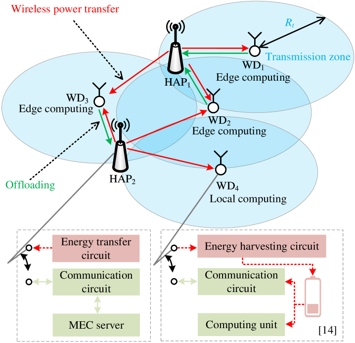
As shown in Fig. 1, we study a WP-MEC network, where one-antenna HAPs, and one-antenna WDs coexist. Let denote the set of HAPs, and denote the set of WDs. Equipped with one MEC server, each HAP broadcasts the RF signal to WDs through the downlink channel, and receives the computation data from WDs through the uplink channel. Equipped with one battery with capacity , each WD harvests energy from RF signals for local computing or offloading the computation data to the chosen HAP. We consider that WDs adopt the harvest-then-offload protocol [15], i.e., WDs harvest energy before offloading data to the HAPs. In accordance with the real demand, we define the transmission zone as a circle centered at the WD with radius . The WD could offload its computation data to the HAPs within the corresponding transmission zone.
To process the generated computation data in the WP-MEC network, we consider that WDs follow the binary offloading policy, i.e., there are two computing modes for WDs. The WD in local computing mode processes the computation data locally by utilizing the computing units, and the WD in edge computing mode offloads the computation data to the chosen HAP through the uplink channel. After receiving the computation data, the HAP processes the received computation data, and transmits computation results back to the WD through the downlink channel.
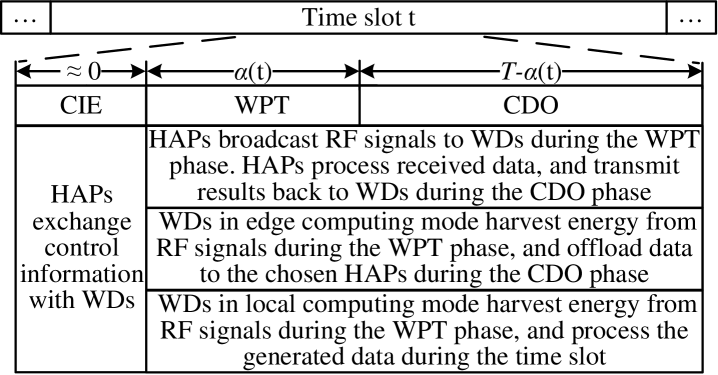
As illustrated in Fig. 2, the system time is divided into time slots with equal duration . Time slot is divided into the control information exchanges (CIE) phase with negligible duration due to small-sized control information [27], the WPT phase with duration , and the computation data offloading (CDO) phase with duration . During the CIE phase, the control information exchanges between HAPs and WDs complete. During the WPT phase, HAPs broadcast RF signals to WDs through the downlink channels, and WDs harvest energy from RF signals of HAPs simultaneously. During the CDO phase, the WDs in edge computing mode offload the computation data to the chosen HAPs through the uplink channels. While the WDs in local computing mode process the computation data during the time slot, since the energy harvesting circuit and the computing unit could work simultaneously [15, 21], as shown in the WD’s circuit structure of Fig. 1. At the beginning of time slot , WDs generate computation data , where respectively denote the amount of the computation data generated by WD1, , WDN at time slot , and WDs transmit the state information about the amount of the generated computation data and the amount of the energy in the batteries to the HAPs. Then the HAPs follow the proposed TMADO framework to output the feasible solutions of the offloading decisions, broadcast them to WDs, and conduct WPT with duration . According to the received feasible solutions of the offloading decisions, each WD independently makes the optimal offloading decision, i.e., it processes the generated computation data locally during the current time slot, or offloads the computation data to the chosen HAP during the CDO phase. To avoid potential interference, the time division multiple access (TDMA) protocol is employed by WDs that offload the computation data to the same HAP at the same time slot, while the frequency division multiple access (FDMA) protocol is employed by WDs that offload the computation data to different HAPs. As the MEC server of the HAP has high CPU frequency [24], there is no competition among WDs for the edge resource. Similarly, as the MEC server of the HAP has high CPU frequency [24] and the computation results are small-sized [15], we neglect the time spent by HAPs on processing data and transmitting the computation results back to the WDs.
II-B Channel Model
For the channels in the WP-MEC network, we adopt the free-space path loss model for the large-scale fading, and adopt the Rayleigh fading model [28] for the small-scale fading. Let denote the channel gain between WDn and HAPm at time slot as
| (1) |
where denotes the large-scale fading component, and denotes the small-scale fading component at time slot . The uplink channel and downlink channel are considered to be symmetric [14], i.e., the channel gain of the uplink channel equals that of the corresponding downlink channel. We consider that channel gains remain unchanged within each time slot, and vary from one time slot to another.
II-C Energy Harvesting Model
During the WPT phase, WDs harvest energy from the RF signals broadcasted by HAPs. The amount of the energy harvested by WDs depends on the transmit power of the HAPs, the distance between WDs and HAPs, and the duration of the WPT phase. We adopt the linear energy harvesting (EH) model, and formulate the amount of the energy harvested by WDn at time slot as
| (2) |
where denotes the EH efficiency, denotes the transmit power of HAPm at time slot , and denotes the maximum transmit power of HAPs.
The amount of the available energy in WDn at time slot , i.e., the sum of the amount of the initial energy in WDn and the amount of the energy harvested by WDn at time slot , is formulated as
| (3) |
where denotes the amount of the initial energy in WDn at time slot . At the beginning of the first time slot, the initial energy in WDs equals zero, i.e., . As shown in (3), ensures that the amount of the available energy in WDn does not exceed the battery capacity. Then the amount of initial energy in WDn at time slot updates as
| (4) |
where denotes the amount of the energy consumed by WDn at time slot .
II-D Offloading Decisions
According to the computing modes, WDs are divided into nonoverlapping sets , , and . Let denote the set of WDs that process the computation data by offloading it to HAPm at time slot , denote the set of WDs that process the computation data locally at time slot , and denote the set of WDs that fail to process the computation data at time slot . If the available energy in WD is not enough for local computing in (9) or edge computing in (13), WD fails to process the computation data at time slot . The WDs failing to process the computation data at time slot are not in the feasible solutions of the offloading decisions from HAPs. Considering the quality of service requirement for the WDs in , the WDs in directly drop the computation data without retransmitting, and accumulate the energy in the batteries so as to successfully process the computation data of the following time slots. varies across time slots since WDs with sufficient harvested energy process the generated computation data locally, or offload it to the chosen HAPs. Then , , and satisfy
| (5) |
where , , , and denotes the empty set.
II-E Local Computing Mode
According to the received feasible solutions of the offloading decisions from HAPs, when WDn chooses local computing mode at time slot , i.e., , it processes the generated computation data of bits locally during the whole time slot. Let with denote the CPU frequency of WDn by using dynamic voltage and frequency scaling technique [29] at time slot , where denotes the maximum CPU frequency of WDs. Let denote the number of CPU cycles required by WDn to process 1-bit data. The computing delay constraint, i.e., the delay of WDn to process the generated computation data at time slot , denoted by , does not exceed the duration of the time slot , is formulated as
| (6) |
Since energy is the product of power and time, the amount of the energy consumed by WDn for local computing at time slot is the product of the CPU power of WDn, denoted by , and the delay of WDn to process the generated computation data, i.e., . According to [30] and [31], the CPU power of WDn at time slot is expressed as
| (7) |
where denotes the switched load capacitance of WDn, and denotes the CPU voltage of WDn at time slot . As pointed out by [31], when the CPU operates at the low voltage limit, which is in accordance with the real-world WDs, the CPU frequency is approximately linear with the CPU voltage. Consequently, in (7) can be reformulated as , where satisfying is called the effective switched load capacitance of WDn [32]. Then the amount of the energy consumed by WDn for local computing at time slot is expressed as
| (8) |
which has been extensively used in the works related to MEC networks [14, 15, 20, 21, 32].
Since WDs in local computing mode are powered by the energy harvested during the WPT phase and that stored in the batteries, the energy constraint for WDn in local computing mode, i.e., the amount of the energy consumed by WDn for local computing at time slot is no larger than the available energy in WDn at time slot , is formulated as [24]
| (9) |
II-F Edge Computing Mode
According to the received feasible solutions of the offloading decisions from HAPs, when WDn chooses edge computing mode at time slot , it offloads the computation data to HAPm, i.e., , . Let denote the duration that WDn offloads the computation data of bits to HAPm at time slot . Then and satisfy
| (10) |
Based on Shannon’s formula [33], to ensure that WDn in edge computing mode successfully offloads the computation data to HAPm during the CDO phase, satisfies
| (11) |
where denotes the uplink bandwidth of each HAP, and represents the communication overhead including the encryption and data header costs [14]. denotes the transmit power of WDn, and denotes the power of the additive white Gaussian noise (AWGN). Besides, there is no interference between multiple WDs in (11) due to the TDMA protocol. Let denote the amount of the energy consumed by WDn for transmitting the computation data of bits to HAPm at time slot as
| (12) |
where denotes the circuit power of WDn. During the CDO phase, the energy constraint for WDn in edge computing mode, i.e., the amount of the energy consumed by WDn for edge computing is no larger than that of the available energy in WDn at time slot , is formulated as
| (13) |
Then the amount of the energy consumed by WDn at time slot is defined as
| (14) |
If the WD fails to process the computation data under the TMADO framework at time slot , its computation data would not be scheduled [23], and equals .
The amount of the energy consumed by HAPm at time slot , denoted by , is formulated as
| (15) |
(15) indicates that the energy provision by HAPs consists of the amount of the energy consumed by HAPs for broadcasting RF signals and the amount of the energy consumed by HAPs for processing the received computation data from WDs. During the WPT phase of time slot , the amount of the energy consumed by HAPm for broadcasting the RF signal, denoted by , is formulated as
| (16) |
During the CDO phase of time slot , the amount of the energy consumed by HAPm for processing the received computation data of bits from the WDs in , denoted by , is formulated as [34]
| (17) |
where represents the energy consumption of HAPm for processing per offloaded bit.
III Problem Formulation
In this section, we formulate the long-term energy provision minimization problem in the multi-HAP WP-MEC network as . Then we adopt Lemmas 1 and 2 to prove that for a single time slot is NP-hard, which makes much more perplexed and challenging.
The total amount of the energy provision by HAPs at time slot , denoted by , is expressed as
| (18) |
We aim to minimize in the long term through optimizing the transmit power of HAPs , the duration of the WPT phase , the offloading decisions , the time allocated to WDs for offloading the computation data to HAPs , and the CPU frequencies of WDs as
| (19a) | ||||
| (19b) | ||||
| (19c) | ||||
| (19d) | ||||
| (19e) | ||||
| (19f) | ||||
| (19g) | ||||
| (19h) | ||||
| (19i) | ||||
| (19j) | ||||
| (19k) | ||||
In , (19b) represents the computation data demand constraint that the total amount of the processed computation data at each time slot is no smaller than the computation data demand . (19c) represents the computing delay constraint for each WD in local computing mode. (19d), (19e), and (19f) respectively represent that the duration of offloading the computation data to HAPm, the duration of the WPT phase, and the sum of the total duration of the offloaded computation data to HAPm and the duration of the WPT phase do not exceed the duration of the time slot. (19g) ensures that the transmit power of each HAP does not exceed the maximum transmit power of HAPs. (19h) represents the energy constraint for each WD in local computing mode [23]. (19i) represents that the amount of the energy consumed by the WD in edge computing mode is no larger than that of the available energy in the WD. (19j) ensures that the CPU frequency of each WD does not exceed the maximum CPU frequency. (19k) ensures that the amount of the available energy in each WD, which is equivalent to the sum of the amount of the initial energy in each WD and that of the energy harvested by each WD, does not exceed the battery capacity.
In the following, we provide a detailed explanation of the NP-hardness of the formulated non-convex MIP problem. As defined in [35], we provide the definition of the non-convex MIP problem as
| (20a) | ||||
| (20b) | ||||
| (20c) | ||||
where denotes the vector of integer variables, denotes the vector of continuous variables, represent the arbitrary functions mapping from to the real numbers, denotes the number of integer variables, denotes the number of continuous variables, and denotes the number of constraints. The MIP problem is considered as a general class of problems, consisting of the convex MIP problem and the non-convex MIP problem. The MIP problem is convex if are convex, and vice versa [35].
Then we explain the NP-hardness of the non-convex MIP problem in this paper. According to (19a)-(19k), the formulated energy provision minimization problem for time slot that optimizes , , , , and , is
| (21a) | ||||
It is observed that (21a) includes integer variables and the non-convex function resulting from the coupling relationship between and . According to the definition of the non-convex MIP problem, the formulated energy provision minimization problem for time slot is a non-convex MIP problem. Then we adopt Lemmas 1-2 to prove this non-convex MIP problem is NP-hard.
Lemma 1
Proof:
Satisfying the constraints in (19b), (19h), and (19j) indicates that WDn satisfies the computation data demand constraint, energy constraint, and CPU frequency constraint. Then is a feasible solution of . With given , , , , , the value of in (16) is determined. Based on (15)-(18), the energy provision by HAPs in with WDn in local computing mode is smaller than that with WDn in edge computing mode. This completes the proof. ∎
Lemma 2
With given , , , , and , for time slot is NP-hard.
Proof:
With given , , , , and , the value of in (16) is determined. Based on (15), for time slot aims to minimize in (17) and (18) by optimizing the offloading decisions . Based on (17), we infer that is independent of . Based on Lemma 1, in the optimal offloading solution of for time slot is determined.
According to the aforementioned analysis, we transform for time slot into the multiple knapsack problem as follows. Treat HAPs as knapsacks with the same load capacity . Treat WDs as items with the weight of itemn equaling the duration that WDn offloads the computation data of bits to the chosen HAP. The value of itemn is equal to the amount of the energy consumed by the chosen HAP for processing the computation data of bits from WDn. Then finding is equivalent to finding the optimal item-assigning solution to minimize the total value of the items assigned to knapsacks. The multiple knapsack problem is NP-hard [36]. This completes the proof. ∎
As aforementioned, is a non-convex MIP problem, and we provide Lemmas 1-2 to demonstrate that this non-convex MIP problem is NP-hard in general. Therefore, it is quite challenging to solve , especially in a distributed manner, i.e., each WD independently makes its optimal offloading decision according to the local observation. Each WD can not capture the state information of other WDs and the HAPs that are located outside the corresponding transmission zone.
IV TMADO Framework
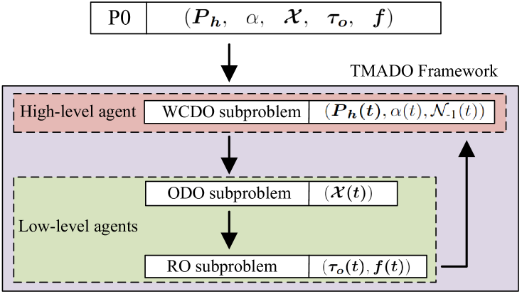
In essence, is a sequential decision-making question. As a power tool for learning effective decisions in dynamic environments, DRL is exploited to tackle . Specifically, as shown in Fig. 3, we propose the TMADO framework to decompose into three subproblems, i.e., WPT and computation data optimization (WCDO) subproblem, offloading decision optimization (ODO) subproblem, and resource optimization (RO) subproblem. We specify the TMADO framework as follows.
-
•
With state information of HAPs, that of WDs, and that of channel gains, the WCDO subproblem optimizes the transmit power of HAPs , duration of the WPT phase , and feasible solutions of the offloading decisions by HAPs, subject to the computation data demand constraint (19b), duration of the WPT phase constraint (19e), and transmit power constraint (19g).
- •
-
•
With the output of the WCDO subproblem {, , }, and the output of the ODO subproblem , the RO subproblem outputs the duration that WDs in edge computing mode offload the computation data to HAPs , and the CPU frequencies of WDs in local computing mode , subject to the computing delay constraints (19c), (19f), and CPU frequency constraint (19j).
The HAPs are considered as a single high-level agent assisted by the server of cloud center in the WCDO subproblem. Each WD is considered as a low-level independent agent in the ODO subproblem. Under the TMADO framework, the decision-making process is completed by both HAPs as the high-level agent and WDs as low-level agents due to the following reasons. 1) Completing the decision-making process by only the high-level agent faces challenges of large-scale output actions and poor scalability. 2) Completing the decision-making process by only low-level agents makes it difficult to determine the duration of the WPT phase and satisfy the computation data demand in (19b). 3) It is difficult to determine the actions output by only high-level agent and those output by only low-level agents due to the coupling relationship between the output of the WCDO subproblem and that of the ODO subproblem.
Based on aforementioned three reasons, we explore a hierarchical structure in the TMADO framework that consists of a single-agent actor-critic architecture based on deep deterministic policy gradient (DDPG), and a multi-agent actor-critic architecture based on independent proximal policy optimization (IPPO). The HAPs first determine the high-level action through the DDPG algorithm. Then each low-level WD updates its own offloading decision through the IPPO algorithm. The states of the high-level agent are influenced by the low-level WDs’ decisions, driving the HAPs to update their actions in the next decision epoch. The TMADO framework performs the control information exchanges between HAPs and WDs during the CIE phase of each time slot as follows. 1) HAPs and WDs transmit states to the high-level agent through the dedicated control channel by using the TDMA protocol. Specifically, HAPs transmit the states of the energy consumption to the high-level agent, and WDs transmit the states of data generation and initial energy to the high-level agent. 2) The high-level agent combines the received states, obtains its action through the high-level learning model, and broadcasts its action to HAPs and WDs. 3) Each low-level agent receives its state, obtains its action through the low-level learning model, and then executes its action.
The WCDO subproblem involves not only the integer variable (i.e., ) but also the continuous variables (i.e., and ). The DDPG does well in searching for the optimal policy with continuous variables for a single agent [37]. Hence the DDPG is employed by the high-level agent at the HAPs to solve the WCDO subproblem. Whereas the ODO subproblem involves only integer variables (i.e., ), and the multi-WD offloading decisions need to be made by the multiple low-level agents at WDs. Different from other multi-agent DRL algorithms such as multi-agent deep deterministic policy gradient (MADDPG), multi-agent deep Q-learning network (MADQN) and multi-agent proximal policy optimization (MAPPO), IPPO estimates individual state value function of each agent without the interference from irrelevant state information of other agents, and then could achieve a better reward [38]. Hence IPPO is employed by the low-level agents at WDs to solve the ODO subproblem.
IV-A WCDO Subproblem
We formulate the WCDO subproblem as a Markov decision process (MDP), represented by a tuple of the high-level agent , where , , , and represent state, action, reward, and the discount factor, respectively. The high-level agent receives state , selects action at time slot , and receives reward and state .
-
•
State space: The global state of the WCDO subproblem at time slot is defined as
(22) where represents the state information of HAPs, represents that of WDs, and represents the channel gains at time slot . is the state information of HAPm that represents the total amount of the energy consumed by HAPm during time slots . represents the amount of the initial energy in WDn at time slot .
-
•
Action space: At time slot , the action space of HAPs is defined as
(23) where represents the energy provision cost of HAPs for the energy supply of WDn estimated by the high-level agent, i.e., the amount of the energy consumed by HAPs for WDn to harvest per joule energy. To be specific, if the energy provision cost of HAPs for the energy supply of WDn is small, the probability that HAPs determine that WDn in local computing mode or edge computing mode processes the computation data is high. Otherwise, the probability that HAPs determine that WDn is not in the feasible solutions of the offloading decisions is high. As is a continuous action, and the feasible solutions of the offloading decisions are discrete actions, we convert continuous action into discrete action, which represents the set of WDs to process the computation data, and obtain . To optimize the feasible solutions of the offloading decisions, the sub-action space is established in the ascending order of action as
(24) The WDs in the feasible solutions of the offloading decisions are powered by HAPs with low energy provision cost, and satisfy (19b). Based on (24), we obtain the feasible solutions of the offloading decisions.
-
•
Reward function: The reward function measures the amount of the energy provision by HAPs at time slot as
(25) where denotes the penalty of dissatisfying (19b). The high-level agent maximizes a series of rewards as
(26)
IV-A1 Architecture Design of the High-level Agent
DDPG is employed by the high-level agent. As the single-agent actor-critic architecture, DDPG uses deep neural networks (DNNs) as a state-action value function to learn the optimal policy in multi-dimensional continuous action space. Let denote the parameters of DNNs, and denote the optimal policy parameters. There are four DNNs in DDPG as follows.
The actor network of the high-level agent with parameters outputs policy . Under policy , the high-level agent adopts state as the input of the actor network to output corresponding action .
The critic network of the high-level agent with parameters evaluates policy generated by the actor network through .
The target actor network and target critic network of the high-level agent are used to improve the learning stability. The structure of the target actor network with parameters is the same as that of the actor network. The structure of the target critic network with parameters is the same as that of the critic network.
The input of the DNNs is state . Motivated by reward in (26), the high-level agent learns the optimal policy with through exploration and training. With obtained optimal policy , the high-level agent chooses the action that maximizes for each state.
IV-A2 Training Process of the High-level Agent
The server of the cloud center assists in training the critic network and actor network of the high-level agent. The experience replay buffer stores the experiences of each time slot. The high-level agent randomly selects -size samples of the experiences, and calculates the loss function of the critic network at time slot as
| (27) |
By the gradient descent method, the parameters of the critic network is updated as
| (28) |
where denotes the learning rate of the critic network.
The action is generated by the actor network of the high-level agent as
| (29) |
where denotes the Gaussian noise at time slot . The Gaussian noise improves the stability and convergence of the actor network [39].
The actor network of the high-level agent aims to maximize the state-action value of the critic network by optimizing the loss function of the actor network as
| (30) |
To achieve the maximum state-action value of the critic network, the gradient ascent method is adopted to update parameters as
| (31) |
where denotes the learning rate of the actor network.
The target actor network and target critic network of the high-level agent update parameters through soft updating as
| (32) |
where and are soft updating factors.
IV-B ODO Subproblem
We formulate the ODO subproblem as a decentralized partially observable Markov decision process (Dec-POMDP), represented by a tuple of low-level agents Pr, where , , , , Pr, and represent states, local observations, actions, rewards, the transition probability, and the discount factor, respectively. As low-level agents, WDs adapt actions to maximize the rewards based on local observations. At the beginning of time slot , the global state of the ODO subproblem is initialized as . At time slot , WDn has observation from state , and then outputs action . The environment receives the set of WDs’ actions , and calculates reward for WDs. Then the environment transites to state according to transition probability Pr.
-
•
State space: The global state of the ODO subproblem at time slot is defined as
(33) where represents the state information of HAPm, represents that of WDn, and represents the channel gains between WDs and HAPm.
-
•
Observation space: denotes the observable state by WDn from the global state of ODO subproblem as
(34) where represents the observation information of HAPm, represents the observation information of WDn, and represents the channel gains between observable WDs and HAPm. The size of for WDn is the same as that of . If HAPm is located outside the transmission zone of WDn, the observation information of HAPm is considered as , and the channel gain between WDn and HAPm is considered as in . As WDn can not capture the observation information of the other WDs, the corresponding observation information of other WDs is considered as for in (34).
-
•
Action space: represents the action space of WDn at time slot . , represents that WDn in edge computing mode offloads the computation data to HAPm at time slot , and represents that WDn in local computing mode processes the computation data locally at time slot .
-
•
Reward function: In view of observation , WDn outputs offloading policy to interact with the environment, and receives reward as
(35) where denotes a constant for the non-negative reward. The value of needs to satisfy two requirements: 1) for ; 2) the value of and those of and are similar in the order of magnitude111We set the value of as the average upper bound of the energy provision by HAPs for the WP-MEC network with a single WD in edge computing mode over all time slots. Namely, when HAPs with the maximum transmit power provide energy for the WD in edge computing mode during time slots, the average value over all time slots, including the energy consumed by HAPs for broadcasting RF signals and that for processing the received computation data from the WD, is defined as (36) where represents the expectation of offloaded bits from WDn at time slot .. The TMADO framework aims to maximize the cumulative sum of (35), i.e., the total reward of low-level agents, by minimizing the energy provision by HAPs in (19a). In the solution of , HAPs only need to provide the required amount of energy for WDs in local computing mode or edge computing mode in (19a).
Based on (22) and (24), HAPs determine the feasible solutions of the offloading decisions , and broadcast them at the beginning of time slot . Then WDs receive the feasible solutions of the offloading decisions, and output actions based on local observations. For WDn, , the ODO subproblem aims to find the optimal policy that maximizes the long-term accumulated discounted reward as
(37) Let denote the parameters of the actor network of low-level agent ,
IV-B1 Architecture Design of Low-level Agents
For the architecture design of low-level agents, IPPO is employed by low-level agents. IPPO, consisting of the actor networks and critic networks, is the multi-agent actor-critic architecture. The number of the actor networks of low-level agents is the same as that of WDs. The actor network of low-level agent with parameters outputs policy , which is predicted distribution of action given local observation . By adding a softmax function [40], the actor network of low-level agent outputs transition probability Pr of WDn’s actions to provide the discrete action, which follows the categorical distribution as
| (38) |
and
| (39) |
where represents the number of WDn’s actions in the action space .
Besides, the number of the critic networks of low-level agents is the same as that of WDs. The critic network of low-level agent with parameters evaluates state value function in (40), and guides the update of the actor network during the training process.
IV-B2 Training Process of Low-level Agents
For the training and execution of low-level agents, centralized training and decentralized execution (CTDE) mechanisms are employed by low-level agents. The CTDE mechanisms do well in tackling the non-stationary issue in multi-agent DRL algorithms by reducing the impact of the interference from irrelevant state information of other agents, and show promising performance in distributed scenarios [41]. To employ CTDE mechanisms, we consider that the server of the cloud center assists in training the critic networks and actor networks of low-level agents in a centralized manner [42], and the trained low-level agents determine actions in a distributed manner. During centralized training, the cloud computing layer has fully-observable access to the states, actions, and rewards of other low-level agents. During decentralized execution, the low-level agent has partially-observable access to the states, actions, and rewards of them, i.e., the low-level agent relies on its local observations to output action for the computation offloading, without the states, actions, and rewards of other WDs.
We introduce the critic networks and actor networks of low-level agents in detail. The critic networks estimate the unknown state value functions to generate update rules for the actor networks. The actor networks output policies to maximize the fitted state values.
The objective function for the critic network of low-level agent at time slot , i.e., the state value function, is formulated as
| (40) |
where is the discount factor. The advantage function of low-level agent at time slot , i.e., comparing the old policy and the current policy in terms of variance, is formulated as
| (41) |
The state value function in (40) is updated by the mean squared error loss function as
| (42) |
Based on (41), the objective function of the actor network of low-level agent at time slot , i.e., the surrogate objective of low-level agent , is formulated as
| (43) |
where represents the truncated importance sampling factor, represents the current policy, represents the old policy, the clip function makes in the value range to train the actor network of low-level agent , and represents a positive hyperparameter. To evaluate the difference between the old and current policies, the surrogate objective of low-level agent uses the importance sampling strategy [40] to treat the samples from the old policy as the surrogate of new samples in training the actor network of low-level agent .
IV-C RO Subproblem
With given {, , , }, we analyze the RO subproblem as follows. We first consider the case when WDn chooses local computing mode at time slot , i.e., .
Lemma 3
With given , , , the optimal computing delay and the CPU frequency of WDn in local computing mode at time slot are respectively given as
| (44) |
and
| (45) |
Proof:
With given , based on (3), the initial energy in WDn at time slot is determined by the initial energy in WDn and the energy consumption of WDn for local computing at time slot . With given , , the amount of the initial energy in WDn at time slot decreases with the amount of the energy consumed by WDn for local computing at time slot , which is given as follows based on (6) and (8).
| (46) |
decreases with . Based on (6) and the monotonicity of with respect to , we have (45). ∎
Then we consider the case when WDn chooses edge computing mode at time slot , i.e., .
Lemma 4
With given , , , the optimal duration that WDn offloads the computation data to HAPm , , at time slot is
| (47) |
Proof:
Based on Lemma 3 and (19i), the amount of the energy consumed by WDn for edge computing is
| (48) |
It is easy to observe that increases with . Based on (11), (19d), (19f), and the monotonicity of with respect to , the minimum duration that WDn offloads the computation data to HAPm in (47) ensures that WDn in edge computing mode successfully offloads the computation data of bits to HAPm. ∎
IV-D Proposed TMADO Framework
Algorithm 1 shows the pseudo-code of the proposed TMADO framework. To be specific, we initialize the actor-critic network parameters of the high-level agent and low-level agents, and the experience replay buffers of the high-level agent and low-level agents in line 1. Then we start a loop for sampling and training in line 2. The high-level agent outputs action by the DDPG algorithm in lines 5-6. After interacting with the environment in line 7, the actions of the high-level agent in (23) are broadcasted to low-level agents, and used as the starting point for low-level agents’ action exploration in line 8. Low-level agents output actions by the IPPO algorithm in lines 10-11. After interacting with the environment in line 12, low-level agent stores the sampled experience and into the experience replay buffer of low-level agent in lines 13-14. The high-level agent stores the sampled experience into the experience replay buffer of the high-level agent in lines 16-17. Then the critic network, the actor network, the target critic network, and the target actor network of the high-level agent are updated in line 18. We update the critic networks and actor networks of low-level agents for times as sample reuse in PPO [38] in lines 20-27. Each time, the experience replay buffer is traversed to conduct mini-batch training.
IV-E Computation Complexity Analysis
We provide the computational complexity analysis of the training process as follows. For the high-level agent, let , , , , and denote the number of layers for the actor network, that for the critic network, the number of neurons in layer of the actor network, the number of neurons in layer of the critic network, and the number of episodes, respectively. Then the complexity of the high-level agent can be derived as [39]. Since low-level agents adopt mini-batches of experience to train policies by maximizing the discounted reward in (37), based on (43), we adopt the sample complexity in [41] to characterize the convergence rate by achieving
| (49) |
Then the sample complexity of low-level agents is [41]. The complexity of solving (44)-(47) is . In summary, the overall computational complexity of the training process is .
V Simulation Results
| Descriptions | Parameters and values |
|---|---|
| = , | |
| , s | |
| Network model | m, mJ |
| , bit | |
| bit | |
| EH model | , W |
| Local computing mode | , cycle/bit, |
| [23] | GHz |
| MHz, W [24] | |
| Edge computing mode | W, W |
| J/bit [34], | |
| High-level agent | , |
| (DDPG) | , , |
| Low-level agents | , |
| (IPPO) | , , |
versus .
TMADO scheme versus training episodes.
In this section, we set the WP-MEC network with the area of 100 m 100 m field [42], where HAPs are uniformly distributed, and WDs are randomly distributed. The distance between WDn and HAPm is , and then the large-scale fading component is [14], where with is the antenna gain, with 915 MHz is the carrier frequency, and with is the path loss exponent. The small-scale Rayleigh fading follows an exponential distribution with unit mean. The number of the arrived data packets in WDs follows an independent Poisson point process with rate . Other simulation parameters are given in TABLE II.
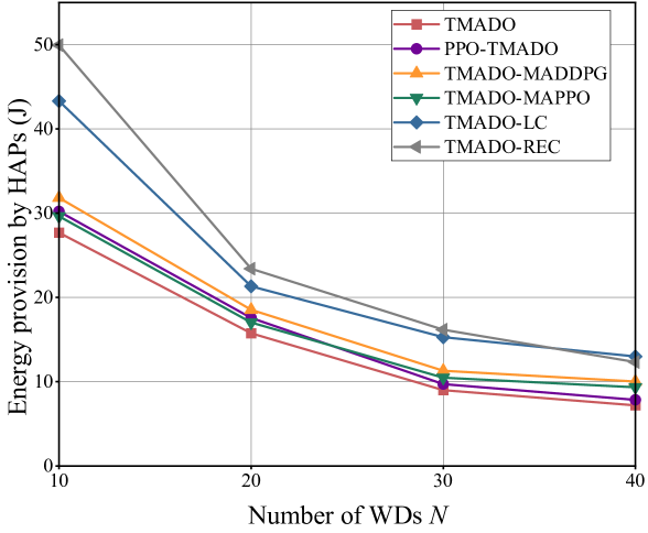
In the following, we first show the convergence of the proposed TMADO scheme in Figs. 6-6 and then reveal the impacts of crucial parameters, such as the number of HAPs/WDs and the radius of the transmission zone, on the energy provision by HAPs in Figs. 9-14. To evaluate the proposed TMADO scheme in terms of the energy provision by HAPs, we provide five comparison schemes as follows.
-
•
Proximal policy optimization (PPO)-TMADO scheme: We use the PPO [43] to obtain , and use the proposed TMADO scheme to obtain
-
•
TMADO-MADDPG scheme: MADDPG is DDPG with the centralized state value function [25]. We use the proposed TMADO scheme to obtain , and use the MADDPG to obtain .
-
•
TMADO-MAPPO scheme: MAPPO is PPO with the centralized state value function [40]. We use the proposed TMADO scheme to obtain , and use the MAPPO to obtain .
-
•
TMADO-random edge computing (REC) scheme: All WDs offload the computation data to random HAPs. We set the radius of the transmission zone m. Besides, we use the proposed TMADO scheme to obtain .
-
•
TMADO-local computing (LC) scheme: All WDs adopt local computing mode. Besides, we use the proposed TMADO scheme to obtain .
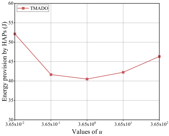
Fig. 6 plots the energy provision (EP) versus . The hyperparameter directly determines the reward of the WD that successfully processes the computation data. Since the number of the arrived data packets in WDn, i.e., , follows an independent Poisson point process with rate in the simulation, the value of in (36) is reformulated as , which is equal to . We observe that reaches the minimum EP, which validates the rationality and superiority of the selected . The reason is that, when is small, WDs tend to select the action of failing to process the computation data, and then HAPs need to provide more energy to satisfy the computation data demand. When is large, WDs tend to select the action of successfully processing the computation data, but are hard to make the offloading decisions, due to the indistinguishableness in the reward of selecting edge computing mode and that of selecting local computing mode. Hence HAPs also need to provide more energy to satisfy the computation data demand.
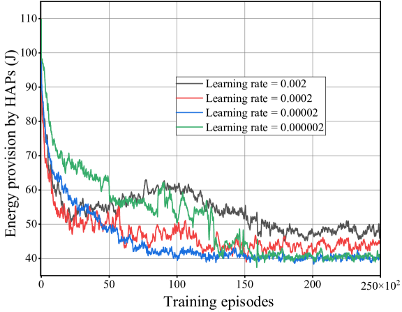
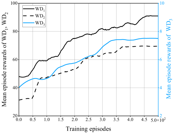
Fig. 6 plots the EP versus training episodes with four values of the learning rate for the high-level agent. We observe that, the proposed TMADO scheme with learning rate achieves smaller EP than that with learning rates and , and converges faster than that with learning rate . Thus we adopt as the learning rate of the high-level agent. Fig. 6 plots the mean episode rewards of WDs versus training episodes. We observe that, the mean episode rewards of WDs converge after 450 training episodes. This observation verifies the advantage of the TMADO scheme for WDs to achieve a stable policy.
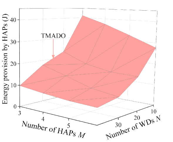
Fig. 9 plots EP under the proposed TMADO scheme versus the number of HAPs and that of WDs . We observe that, EP decreases with . This is due to the reason that, the increase of means that more WDs could harvest energy from HAPs, and accordingly more WDs have sufficient energy to process the computation data in local computing mode or edge computing mode. Thus, with fixed , HAPs could provide less energy for WDs to satisfy computing delay and computation data demand constraints. We also observe that, EP decreases with . This is due to the reason that, the increase of reduces the average distance between HAPs and WDs, and increases the probability that WDs successfully process the computation data in edge computing mode. Thus HAPs could provide less energy for WDs to satisfy computing delay and computation data demand constraints.
TMADO scheme versus the number
of HAPs and that of WDs .
versus the number of WDs with .
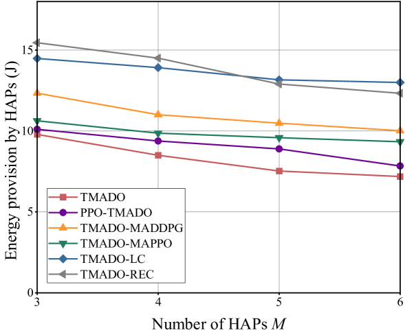
versus the number of HAPs with .
versus the transmission bandwidth .
versus the computation data demand .
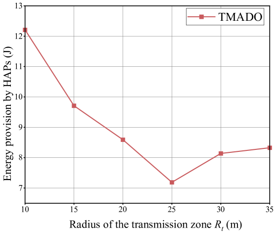
Fig. 9 and Fig. 9 plot EP under six schemes versus the number of WDs with the number of HAPs , and EP versus the number of HAPs with the number of WDs , respectively. We observe that, the proposed TMADO scheme achieves the minimum EP compared with other comparison schemes, which validates the superiority of the proposed TMADO scheme in terms of EP. This is due to the reason that, the DDPG takes advantage of learning continuous policies to solve the WCDO subproblem, while the IPPO employs the individual state value function of each WD to reduce the impact of interference from irrelevant state information of other WDs, which is better for solving the ODO subproblem than the algorithms with the centralized state value function of WDs, i.e., the MADDPG and MAPPO. We also observe that, EP under the TMADO-REC scheme is larger than that under the TMADO-LC scheme for in Fig. 9 and in Fig. 9, but is smaller than that under the TMADO-LC scheme for in Fig. 9 and in Fig. 9. This is due to the reason that, when or is small, the average distance between HAPs and WDs is large. Then WDs under the TMADO-REC scheme would need more energy to offload the computation data to random HAPs to satisfy computing delay and computation data demand constraints. While when or is large, the average distance between HAPs and WDs would be small, which increases the number of accessible HAPs to WDs. Accordingly, HAPs could provide less energy for WDs under the TMADO-REC scheme to satisfy computing delay and computation data demand constraints.
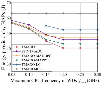
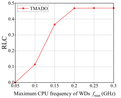
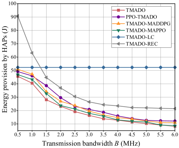
Fig. 12 plots EP versus the transmission bandwidth . We observe that, EP under the proposed TMADO scheme is the minimum, which validates the advantage of the proposed TMADO scheme in terms of EP. We also observe that, EP under the TMADO-LC scheme remains unchanged with the transmission bandwidth, and EP under the other schemes decreases with the transmission bandwidth. This is due to the reason that, the increase of the transmission bandwidth shortens the duration that WDs offload the computation data to HAPs, and decreases the amount of the energy consumed by WDs in edge computing mode. As edge computing mode is not considered in the TMADO-LC scheme, EP under the TMADO-LC scheme remains unchanged with the offloading bandwidth.
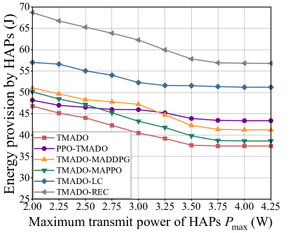
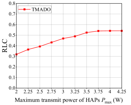
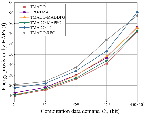
Fig. 12 plots EP versus the computation data demand . We observe that, EP increases with . With higher value of , WDs need to process larger amount of computation data in local computing mode or edge computing mode and make more offloading decisions, which requires more EP.
Fig. 12 plots EP versus the radius of the transmission zone . We observe that, EP first decreases with and then increases with . Apparently, the value of not only influences the number of accessible HAPs to WDs but also the observation space of low-level agents at WDs, and both of them increase with . When is small, the accessible HAPs are not enough for WDs to find the optimal offloading decisions, and then the number of accessible HAPs to WDs is the key factor influencing the EP by HAPs. Hence the EP by HAPs first decreases with . When is large, more HAPs far away from WDs are included in the transmission zones, which means that more redundant observation information is included in the observation space of WDs, i.e., in Section IV-B. Although the accessible HAPs are enough for WDs to find the optimal offloading decisions, the observation space of WDs, i.e., in Section IV-B, also becomes large, which in turn causes that the low-level agents at WDs are difficult to find the optimal offloading decisions. Hence, the EP by HAPs then increases with .
Fig. 13 (a) plots EP versus the maximum CPU frequency of WDs . We observe that, EP under the TMADO-REC scheme remains unchanged, and EP under the other schemes decreases with the maximum CPU frequency of WDs for GHz, and remains unchanged with the maximum CPU frequency of WDs for GHz. This is due to the reason that, WDs under the TMADO-REC scheme are always in edge computing mode, and the energy consumption is independent of the maximum CPU frequency of WDs. Besides, when is small, the computing delay constraint for WDs in local computing mode can not be satisfied, and is the bottleneck limiting WDs to choose local computing mode. With the increase of , WDs have higher probabilities to choose local computing mode, i.e., the ratio of the number of WDs in local computing mode to the total number of WDs that process computation data (RLC) becomes larger, as shown in Fig. 13 (b). Hence EP first decreases with . However, when reaches a certain value such as GHz in Fig. 13 (a), the optimal in (45) is in the range of , and the RLC is no longer affected by , as shown in Fig. 13 (b). Hence EP keeps unchanged. We also observe that, EP with GHz under the TMADO-LC scheme is not shown in Fig. 13 (a), due to the reason that WDs with small can not satisfy the computing delay constraint and the computation data demand .
Fig. 14 (a) plots EP versus the maximum transmit power of HAPs . We observe that, the proposed TMADO scheme achieves the minimum EP compared with comparison schemes. We also observe that, EP first decreases and then keeps unchanged with the maximum transmit power of HAPs . The reason is that, when is small, such as W in Fig. 14 (a), WDs are in the energy-deficit state. In such a context, it is best for HAPs to transmit RF signals with the maximum transmit power , so that WDs harvest more energy to have more choices, i.e., local computing mode or edge computing mode. Actually, the WDs with more energy, such as the WDs close to HAPs (i.e., with high channel gains), prefer local computing so as to avoid the energy consumption by HAPs for processing the offloaded computation data. While the WDs with less energy, such as the WDs far away from HAPs (i.e., with low channel gains), can not support local computing and have to offload the computation data to HAPs. Then HAPs consume their energy to process the computation data. With the increase of , WDs harvest larger amount of energy. More WDs, especially the WDs with high channel gains, have sufficient energy to perform local computing, which is beneficial to reduce the EP by HAPs for processing the offloaded computation data. Hence the RLC increases with , as shown in Fig. 14 (b). Accordingly, EP first decreases with . When reaches a certain value, i.e., W in Fig. 14 (a), WDs have two modes to process the computation data, and the optimal transmit power of HAPs is not the maximum. Hence EP keeps unchanged for W.
VI Conclusion
This paper studied the long-term energy provision minimization problem in a dynamic multi-HAP WP-MEC network under the binary offloading policy. We mathematically formulated the optimization problem by jointly optimizing the transmit power of HAPs, the duration of the WPT phase, the offloading decisions of WDs, the time allocation for offloading and the CPU frequency for local computing, subject to the energy, computing delay and computation data demand constraints. To efficiently address the formulated problem in a distributed way, we proposed a TMADO framework with which each WD could optimize its offloading decision, time allocation for offloading and CPU frequency for local computing. Simulation results showed that the proposed TMADO framework achieves a better performance in terms of the energy provision by comparing with other five comparison schemes. This paper investigated the fundamental scenario with single-antenna HAPs. As one of the future research directions, we will further study the scenario with multi-antenna HAPs by jointly considering the beamforming technique and channel allocation.
References
- [1] Y. Chen, Y. Sun, B. Yang, and T. Taleb, “Joint caching and computing service placement for edge-enabled IoT based on deep reinforcement learning,” IEEE Internet Things J., vol. 9, no. 19, pp. 19501–19514, Oct. 2022.
- [2] X. Wang, J. Li, Z. Ning, Q. Song, L. Guo, S. Guo, and M. S. Obaidat, “Wireless powered mobile edge computing networks: A survey,” ACM Comput. Surv., vol. 55, no. 13, pp. 1–37, Jul. 2023.
- [3] K. Wang, J. Jin, Y. Yang, T. Zhang, A. Nallanathan, C. Tellambura, and B. Jabbari, “Task offloading with multi-tier computing resources in next generation wireless networks,” IEEE J. Sel. Areas Commun., vol. 41, no. 2, pp. 306–319, Feb. 2023.
- [4] S. Yue, J. Ren, N. Qiao, Y. Zhang, H. Jiang, Y. Zhang, and Y. Yang, “TODG: Distributed task offloading with delay guarantees for edge computing,” IEEE Trans. Parallel Distrib. Syst., vol. 33, no. 7, pp. 1650–1665, Jul. 2022.
- [5] X. Qiu, W. Zhang, W. Chen, and Z. Zheng, “Distributed and collective deep reinforcement learning for computation offloading: A practical perspective,” IEEE Trans. Parallel Distrib. Syst., vol. 32, no. 5, pp. 1085–1101, May 2021.
- [6] Z. Wang, X. Mu, Y. Liu, X. Xu, and P. Zhang, “NOMA-aided joint communication, sensing, and multi-tier computing systems,” IEEE J. Sel. Areas Commun., vol. 41, no. 3, pp. 574–588, Mar. 2023.
- [7] G. Fragkos, N. Kemp, E. E. Tsiropoulou, and S. Papavassiliou, “Artificial intelligence empowered UAVs data offloading in mobile edge computing,” in Proc. IEEE Int. Conf. Commun., Dublin, Ireland, Jun. 2020, pp. 1-7.
- [8] P. A. Apostolopoulos, G. Fragkos, E. E. Tsiropoulou, and S. Papavassiliou, “Data offloading in UAV-assisted multi-access edge computing systems under resource uncertainty,” IEEE Trans. Mobile Comput., vol. 22, no. 1, pp. 175–190, Jan. 2023.
- [9] H. Dai, Y. Xu, G. Chen, W. Dou, C. Tian, X. Wu, and T. He, “ROSE: Robustly safe charging for wireless power transfer,” IEEE Trans. Mobile Comput., vol. 21, no. 6, pp. 2180–2197, Jun. 2022.
- [10] Y. Wu, Y. Song, T. Wang, L. Qian, and T. Q. S. Quek, “Non-orthogonal multiple access assisted federated learning via wireless power transfer: A cost-efficient approach,” IEEE Trans. Commun., vol. 70, no. 4, pp. 2853-2869, Apr. 2022.
- [11] X. Liu, B. Xu, K. Zheng, and H. Zheng, “Throughput maximization of wireless-powered communication network with mobile access points,” IEEE Trans. Wireless Commun., vol. 22, no. 7, pp. 4401–4415, Jul. 2023.
- [12] X. Liu, H. Liu, K. Zheng, J. Liu, T. Taleb, and N. Shiratori, “AoI-minimal clustering, transmission and trajectory co-design for UAV-assisted WPCNs,” IEEE Trans. Veh. Technol., early access, Sep. 16, 2024, doi: 10.1109/TVT.2024.3461333.
- [13] X. Deng, J. Li, L. Shi, Z. Wei, X. Zhou, and J. Yuan, “Wireless powered mobile edge computing: Dynamic resource allocation and throughput maximization,” IEEE Trans. Mobile Comput., vol. 21, no. 6, pp. 2271–2288, Jun. 2022.
- [14] S. Bi and Y. J. Zhang, “Computation rate maximization for wireless powered mobile-edge computing with binary computation offloading,” IEEE Trans. Wireless Commun., vol. 17, no. 6, pp. 4177–4190, Jun. 2018.
- [15] F. Zhou and R. Q. Hu, “Computation efficiency maximization in wireless-powered mobile edge computing networks,” IEEE Trans. Wireless Commun., vol. 19, no. 5, pp. 3170–3184, May 2020.
- [16] X. Chen, W. Dai, W. Ni, X. Wang, S. Zhang, S. Xu, and Y. Sun, “Augmented deep reinforcement learning for online energy minimization of wireless powered mobile edge computing,” IEEE Trans. Commun., vol. 71, no. 5, pp. 2698–2710, May 2023.
- [17] J. Park, S. Solanki, S. Baek, and I. Lee, “Latency minimization for wireless powered mobile edge computing networks with nonlinear rectifiers,” IEEE Trans. Veh. Technol., vol. 70, no. 8, pp. 8320–8324, Aug. 2021.
- [18] F. Wang, J. Xu, and S. Cui, “Optimal energy allocation and task offloading policy for wireless powered mobile edge computing systems,” IEEE Trans. Wireless Commun., vol. 19, no. 4, pp. 2443–2459, Apr. 2020.
- [19] S. Zeng, X. Huang, and D. Li, “Joint communication and computation cooperation in wireless-powered mobile-edge computing networks with NOMA,” IEEE Internet Things J., vol. 10, no. 11, pp. 9849–9862, Jun. 2023.
- [20] Y. Ye, L. Shi, X. Chu, R. Q. Hu, and G. Lu, “Resource allocation in backscatter-assisted wireless powered MEC networks with limited MEC computation capacity,” IEEE Trans. Wireless Commun., vol. 21, no. 12, pp. 10678–10694, Dec. 2022.
- [21] J. Du, H. Wu, M. Xu, and R. Buyya, “Computation energy efficiency maximization for NOMA-based and wireless-powered mobile edge computing with backscatter communication,” IEEE Trans. Mobile Comput., vol. 23, no. 6, pp. 6954–6970, Jun. 2024.
- [22] S. Zhang, S. Bao, K. Chi, K. Yu, and S. Mumtaz, “DRL-based computation rate maximization for wireless powered multi-AP edge computing,” IEEE Trans. Commun., vol. 72, no. 2, pp. 1105–1118, Feb. 2024.
- [23] X. Wang, Z. Ning, L. Guo, S. Guo, X. Gao, and G. Wang, “Online learning for distributed computation offloading in wireless powered mobile edge computing networks,” IEEE Trans. Parallel Distrib. Syst., vol. 33, no. 8, pp. 1841–1855, Aug. 2022.
- [24] F. Wang, J. Xu, X. Wang, and S. Cui, “Joint offloading and computing optimization in wireless powered mobile-edge computing systems,” IEEE Trans. Wireless Commun., vol. 17, no. 3, pp. 1784–1797, Mar. 2018.
- [25] H. Zhou, Y. Long, S. Gong, K. Zhu, D. T. Hoang, and D. Niyato, “Hierarchical multi-agent deep reinforcement learning for energy-efficient hybrid computation offloading,” IEEE Trans. Veh. Technol., vol. 72, no. 1, pp. 986–1001, Jan. 2023.
- [26] G. Hong, B. Yang, W. Su, H. Li, Z. Huang, and T. Taleb, “Joint content update and transmission resource allocation for energy-efficient edge caching of high definition map,” IEEE Trans. Veh. Technol., vol. 73, no. 4, pp. 5902–5914, Apr. 2024.
- [27] Q. Shafiee, Č. Stefanović, T. Dragičević, P. Popovski, J. C. Vasquez, and J. M. Guerrero, “Robust networked control scheme for distributed secondary control of islanded microgrids,” IEEE Trans. Ind. Electron., vol. 61, no. 10, pp. 5363–5374, Oct. 2014.
- [28] R. Sun, H. Wu, B. Yang, Y. Shen, W. Yang, X. Jiang, and T. Taleb, “On covert rate in full-duplex D2D-enabled cellular networks with spectrum sharing and power control,” IEEE Trans. Mobile Comput., early access, Mar. 8, 2024, doi: 10.1109/TMC.2024.3371377.
- [29] S. Barbarossa, S. Sardellitti, and P. Di Lorenzo, “Communicating while computing: Distributed mobile cloud computing over 5G heterogeneous networks,” IEEE Signal Process. Mag., vol. 31, no. 6, pp. 45–55, Nov. 2014.
- [30] C.-L. Su, C.-Y. Tsui, and A. Despain, “Low power architecture design and compilation techniques for high-performance processors,” in Proc. IEEE COMPCON, San Francisco, CA, USA, Feb. 1994, pp. 489–498.
- [31] T. D. Burd and R. W. Brodersen, “Processor design for portable systems,” J. VLSI Signal Process. Syst., vol. 13, no. 2, pp. 203–221, Aug. 1996.
- [32] L. T. Hoang, C. T. Nguyen, and A. T. Pham, “Deep reinforcement learning-based online resource management for UAV-assisted edge computing with dual connectivity,” IEEE/ACM Trans. Netw., vol. 31, no. 6, pp. 2761–2776, Dec. 2023.
- [33] H. Li, K. Xiong, Y. Lu, B. Gao, P. Fan, and K. B. Letaief, “Distributed design of wireless powered fog computing networks with binary computation offloading,” IEEE Trans. Mobile Comput., vol. 22, no. 4, pp. 2084–2099, Apr. 2023.
- [34] T. Bai, C. Pan, H. Ren, Y. Deng, M. Elkashlan, and A. Nallanathan, “Resource allocation for intelligent reflecting surface aided wireless powered mobile edge computing in OFDM systems,” IEEE Trans. Wireless Commun., vol. 20, no. 8, pp. 5389–5407, Aug. 2021.
- [35] S. Burer and A. N. Letchford, “Non-convex mixed-integer nonlinear programming: A survey,” Surv. Oper. Res. Manage. Sci., vol. 17, no. 2, pp. 97–106, Jul. 2012.
- [36] V. Cacchiani, M. Iori, A. Locatelli, and S. Martello, “Knapsack problems — An overview of recent advances. Part II: Multiple, multidimensional, and quadratic knapsack problems,” Comput. Operations Res., vol. 143, p. 105693, Jul. 2022.
- [37] Y. Yu, J. Tang, J. Huang, X. Zhang, D. K. C. So, and K.-K. Wong, “Multi-objective optimization for UAV-assisted wireless powered IoT networks based on extended DDPG algorithm,” IEEE Trans. Commun., vol. 69, no. 9, pp. 6361–6374, Jun. 2021.
- [38] Y. Ye, C. H. Liu, Z. Dai, J. Zhao, Y. Yuan, G. Wang, and J. Tang, “Exploring both individuality and cooperation for air-ground spatial crowdsourcing by multi-agent deep reinforcement learning,” in Proc. Int. Conf. Data Eng., Anaheim, CA, USA, Apr. 2023, pp. 205–217.
- [39] K. Zheng, R. Luo, Z. Wang, X. Liu, and Y. Yao, “Short-term and long-term throughput maximization in mobile wireless-powered Internet of Things,” IEEE Internet Things J., vol. 11, no. 6, pp. 10575–10591, Mar. 2024.
- [40] Z. Hao, G. Xu, Y. Luo, H. Hu, J. An, and S. Mao, “Multi-agent collaborative inference via DNN decoupling: Intermediate feature compression and edge learning,” IEEE Trans. Mobile Comput., vol. 22, no. 10, pp. 6041–6055, Oct. 2023.
- [41] Hairi, J. Liu, and S. Lu, “Finite-time convergence and sample complexity of multi-agent actor-critic reinforcement learning with average reward,” in Proc. Int. Conf. Learn. Represent., Virtual, Oct. 2022, pp. 25–29.
- [42] Z. Gao, L. Yang, and Y. Dai, “Large-scale computation offloading using a multi-agent reinforcement learning in heterogeneous multi-access edge computing,” IEEE Trans. Mobile Comput., vol. 22, no. 6, pp. 3425–3443, Jun. 2023.
- [43] Y. Wang, M. Chen, T. Luo, W. Saad, D. Niyato, H. V. Poor, and S. Cui, “Performance optimization for semantic communications: An attention-based reinforcement learning approach,” IEEE J. Sel. Areas Commun., vol. 40, no. 9, pp. 2598–2613, Sep. 2022.