Distributed Convex Optimization with State-Dependent (Social) Interactions over Random Networks

Distributed multi-agent optimization has been an attractive topic due to its applications in several areas such as power systems, smart buildings, and machine learning to name a few; therefore, several investigators have paid much attention to distributed optimization problems (see Surveys [1]-[4]). Switched dynamical systems are divided into two categories: arbitrary (or state-independent) and state-dependent (see [5] and references therein for details and several examples). Many references, cited in Surveys [1]-[4], have investigated distributed optimization over arbitrary networks.

On the other hand, state-dependent networks have been shown in practical systems such as flocking of birds [6], opinion dynamics [7]-[15], mobile robotic networks [16], wireless networks [17], and predator-prey interaction [18]. For example, an agent in social networks weighs the opinions of others based on how much its opinion is close to theirs (see Section I in the preliminary version, i.e., [31], for more details).

In state-dependent networks, coupling between algorithm analysis and information exchange among agents impose significant challenge because states of agents at each time determine the weights in the communication networks. Hence, distributed algorithms’ design for consensus and optimization over state-dependent networks is still a challenge.

Consensus problem for opinion dynamics has been investigated in [7]-[15]. Existence of consensus in a multi-robot network has been shown in [19]. Distributed consensus [21]-[26] and distributed optimization [20], [27]-[29] over state-dependent networks with time-invariant or time-varying¹¹1The underlying communication graph is a priori known in a time-varying arbitrary network at each time $t$, whereas it is a priori unknown in a random arbitrary network. arbitrary graphs have been considered. Hence, the gap in the literature is to consider distributed multi-agent optimization problems with both state-dependent interactions and random arbitrary (see footnote 1) networks.

This paper aims at distributed multi-agent convex optimization over both state-dependent and random arbitrary networks, that has not been addressed in the literature. Assuming doubly stochasticity of weighted matrix of the graph with respect to state variables for each communication network and strong connectivity of the union of the communication networks allows this result to be applicable to periodic and irreducible weighted matrix of the graph in synchronous²²2In a synchronous protocol, all nodes activate at the same time and perform communication updates. On the other hand, in an asynchronous protocol, each node has its concept of time defined by a local timer, which randomly triggers either by the local timer or by a message from neighboring nodes. The algorithms guaranteed to work with no a priori bound on the time for updates are called totally asynchronous, and those that need the knowledge of a priori bound, known as B-connectivity assumption, are called partially asynchronous (see [32] and [33, Ch. 6-7]). protocol. We show that state-dependent weighted random operator of the graph is quasi-nonexpansive³³3It has been shown in [30] that state-independent weighted random operator of the graph has nonexpansivity property.; therefore, imposing a priori distribution of random communication topologies in not required. Thus, it contains random arbitrary networks with/without asynchronous protocols for more general class of switched networks. As an extension of the the distributed optimization problem, we provide a more general mathematical optimization problem than that defined in [30], namely minimization of a convex function over the fixed-value point set of a quasi-nonexpansive random operator. Consequently, the reduced optimization problem to distributed optimization includes both state-independent and state-dependent networks over random arbitrary communication graphs with/without asynchronous protocol (see footnote 3). We prove that the discrete-time algorithm proposed in [30] is utilized for quasi-nonexpansive random operators (which include nonexpansive random operators as a special case). The algorithm converges both almost surely and in mean square to the global optimal solution of the optimization problem under suitable assumptions. For the distributed optimization problem, the algorithm reduces to a totally asynchronous algorithm (see footnote 2). It should be noted that the distributed algorithm⁴⁴4We require to clarify that the distributed algorithm in this paper is the randomized version of the algorithm presented in [29]. In [29], the convergence under deterministic arbitrary switching (see footnote 1) is provided, while we prove here its stochastic convergence (both almost sure and mean square) under random arbitrary switching. Furthermore, quasi-nonexpansivity property of the state-dependent weighted operator of the graph (defined in [29]) has not been shown in [29], whereas we show it here. is totally asynchronous but not asynchronous due to synchronized diminishing step size. The algorithm is able to converge even if the weighted matrix of the graph is periodic and irreducible under synchronous protocol. We provide a numerical example where there is distribution dependency among random arbitrary switching graphs and apply the distributed algorithm to validate the results, while no existing references can conclude results (see Example 1). This version provides proofs, mean square convergence of the proposed algorithm, a numerical example, and larger range of a parameter (i.e., $\beta$) in the algorithm, that have not been presented in the preliminary version (i.e., [31]).

This paper is organized as follows. In Section 2, preliminaries on convex analysis and stochastic convergence are given. In Section 3, formulations of the distributed optimization problem and the mathematical optimization are provided. Algorithm and its convergence analysis are presented in Section 4. Finally, a numerical example is given in order to show advantages of the results in Section 5, followed by conclusions and future work in Section 6.

Notations: $\Re$ denotes the set of all real numbers. For any vector $z\in\Re^{n},\|z\|_{2}=\sqrt{z^{T}z},$ and for any matrix $Z\in\Re^{n\times n},\|Z\|_{2}=\sqrt{\lambda_{\max}(Z^{T}Z)}=\sigma_{\max}(Z)$ where $Z^{T}$ represents the transpose of matrix $Z$, $\lambda_{\max}$ represents maximum eigenvalue, and $\sigma_{\max}$ represents largest singular value. Sorted in an increasing order with respect to real parts, $\lambda_{2}(Z)$ represents the second eigenvalue of a matrix $Z$. $Re(r)$ represents the real part of the complex number $r$. For any matrix $Z\in\Re^{n\times n}$ with $Z=[z_{ij}]$, $\|Z\|_{1}=\max_{1\leq j\leq n}\{\sum_{i=1}^{n}|z_{ij}|\}$ and $\|Z\|_{\infty}=\max_{1\leq i\leq n}\{\sum_{j=1}^{n}|z_{ij}|\}$. $I_{n}$ represents Identity matrix of size $n\times n$ for some $n\in\mathbb{N}$ where $\mathbb{N}$ denotes the set of all natural numbers. $\nabla f(x)$ denotes the gradient of the function $f(x)$. $\otimes$ denotes the Kronecker product. $\times$ represents Cartesian product. $E[x]$ denotes Expectation of the random variable $x$.

A vector $v\in\Re^{n}$ is said to be a stochastic vector when its components $v_{i},i=1,2,...,n$, are non-negative and their sum is equal to 1; a square $n\times n$ matrix $V$ is said to be a stochastic matrix when each row of $V$ is a stochastic vector. A square $n\times n$ matrix $V$ is said to be doubly stochastic matrix when both $V$ and $V^{T}$ are stochastic matrices.

Let $\mathcal{H}$ be a real Hilbert space with norm $\|.\|$ and inner product $\langle.,.\rangle$. An operator $A:\mathcal{H}\longrightarrow\mathcal{H}$ is said to be monotone if $\langle x-y,Ax-Ay\rangle\geq 0$ for all $x,y\in\mathcal{H}$. $A:\mathcal{H}\longrightarrow\mathcal{H}$ is $\rho$-strongly monotone if $\langle x-y,Ax-Ay\rangle\geq\rho\|x-y\|^{2}$ for all $x,y\in\mathcal{H}$. A differentiable function $f:\mathcal{H}\longrightarrow\Re$ is $\rho$-strongly convex if $\langle x-y,\nabla f(x)-\nabla f(y)\rangle\geq\rho\|x-y\|^{2}$ for all $x,y\in\mathcal{H}$. Therefore, a function is $\rho$-strongly convex if its gradient is $\rho$-strongly monotone. A convex differentiable function $f:\mathcal{H}\longrightarrow\Re$ is $\mathcal{L}$-strongly smooth if

A mapping $B:\mathcal{H}\longrightarrow\mathcal{H}$ is said to be $K$-Lipschitz continuous if there exists a $K>0$ such that $\|Bx-By\|\leq K\|x-y\|$ for all $x,y\in\mathcal{H}$. Let $S$ be a nonempty subset of a Hilbert space $\mathcal{H}$ and $Q:S\longrightarrow\mathcal{H}$. The point $x$ is called a fixed point of $Q$ if $x=Q(x)$. And, $\text{Fix}(Q)$ denotes the set of all fixed points of $Q$.

Let $\omega^{*}$ and $\omega$ denote elements in the sets $\Omega^{*}$ and $\Omega$, respectively, where $\Omega=\Omega^{*}\times\Omega^{*}\ldots$. Let $(\Omega^{*},\sigma)$ be a measurable space ($\sigma$-sigma algebra) and $C$ be a nonempty subset of a Hilbert space $\mathcal{H}$. A mapping $x:\Omega^{*}\longrightarrow\mathcal{H}$ is measurable if $x^{-1}(U)\in\sigma$ for each open subset $U$ of $\mathcal{H}$. The mapping $T:\Omega^{*}\times C\longrightarrow\mathcal{H}$ is a random map if for each fixed $z\in C$, the mapping $T(.,z):\Omega^{*}\longrightarrow\mathcal{H}$ is measurable, and it is continuous if for each $\omega^{*}\in\Omega^{*}$ the mapping $T(\omega^{*},.):C\longrightarrow\mathcal{H}$ is continuous.

Note that if $\|T(\omega^{*},x)-T(\omega^{*},x)\|\leq\gamma\|x-y\|,0\leq\gamma<1,$ holds in (1), the operator is called (Banach) contraction.

The Cucker-Smale weight [6], which depends on distance between two agents $i$ and $j$, is of the form

where $Q,\sigma>,$ and $\beta\geq 0$.

In social networks, an agent weighs the opinions of others based on how close its opinion (or state) and theirs are, that motivates consideration of state-dependent networks. Vehicular platoon can be modeled as both position-dependent (or state-dependent by considering the position as state) and random arbitrary networks, that is a practical example for motivation of this work. Therefore, there are two combined networks: 1) a network induced by states’ weights, and 2) the underlying random arbitrary network (see Section III in the preliminary version, i.e., [31], for details). The combined state-dependent & random arbitrary network is formulated as follows.

A network of $m\in\mathbb{N}$ nodes labeled by the set $\mathcal{V}=\{1,2,...,m\}$ is considered. The topology of the interconnections among nodes is not fixed but defined by a set of graphs $\mathcal{G}(\omega^{*})=(\mathcal{V},\mathcal{E}(\omega^{*}))$ where $\mathcal{E}(\omega^{*})$ is the ordered edge set $\mathcal{E}(\omega^{*})\subseteq\mathcal{V}\times\mathcal{V}$ and $\omega^{*}\in\Omega^{*}$ where $\Omega^{*}$ is the set of all possible communication graphs, i.e., $\Omega^{*}=\{\mathcal{G}_{1},\mathcal{G}_{2},...,\mathcal{G}_{\bar{N}}\}$. We assume that $(\Omega^{*},\sigma)$ is a measurable space where $\sigma$ is the $\sigma$-algebra on $\Omega^{*}$. We write $\mathcal{N}_{i}^{in}(\omega^{*})/\mathcal{N}_{i}^{out}(\omega^{*})$ for the labels of agent $i$’s in/out neighbors at graph $\mathcal{G}(\omega^{*})$ so that there is an arc in $\mathcal{G}(\omega^{*})$ from vertex $j/i$ to vertex $i/j$ only if agent $i$ receives/sends information from/to agent $j$. We write $\mathcal{N}_{i}(\omega^{*})$ when $\mathcal{N}_{i}^{in}(\omega^{*})=\mathcal{N}_{i}^{out}(\omega^{*})$. It is assumed that there are no communication delay or communication noise in the network.

It should be noted that in our formulation, the in and out neighbors of each agent $i\in\mathcal{V}$ at each graph $\mathcal{G}_{i}\in\Omega^{*},i=1,\ldots,\bar{N},$ are fixed, and we will consider that the weights of links are possibly state-dependent. For instance, an agent pays attention arbitrarily at each time to its friends while it weighs the difference between its opinion and others for decision (see [29, Sec. III] for more details).

We associate for each node $i\in\mathcal{V}$ a convex cost function $f_{i}:\Re^{n}\longrightarrow\Re$ which is only observed by node $i$. The objective of each agent is to find a solution of the following optimization problem:

where $s\in\Re^{n}$. Since each node $i$ knows only its own $f_{i}$, the nodes cannot individually calculate the optimal solution and, therefore, must collaborate to do so.

The above problem can be formulated based on local variables of the agents as

where $x=[x_{1}^{T},x_{2}^{T},\ldots,x_{m}^{T}]^{T},x_{i}\in\Re^{n},i\in\mathcal{V}$, and the constraint set is reached through state-dependent interactions and random (arbitrary) communication graphs. The set

is known as consensus subspace which is a convex set. Note that the Hilbert space considered in this paper for the distributed optimization problem is $\mathcal{H}=(\Re^{mn},\|.\|_{2}).$

We show $W(\omega^{*},x):=\mathcal{W}(\omega^{*},x)\otimes I_{n}$ and $\mathcal{W}(\omega^{*},x)=[\mathcal{W}_{ij}(\omega^{*},x_{i},x_{j})]$ for the state-dependent weighted matrix of the fixed graph $\omega^{*}\in\Omega^{*}$ in a switching network having all possible communication topologies in the set $\Omega^{*}$. For instance, if nodes are not activated at some time $\tilde{t}$ for communication updates in asynchronous protocol, and/or there are no edges in occuring graph at the time $\tilde{t}$, then $\mathcal{W}(\omega^{*}_{\tilde{t}},x_{\tilde{t}})=I_{m}$.

Now we impose Assumptions 1 and 2 below on $\mathcal{W}(\omega^{*},x)$.

i) $\sum_{j\in\mathcal{N}_{i}^{in}(\omega^{*})\cup\{i\}}\mathcal{W}_{ij}(\omega^{*},x_{i},x_{j})=1,i=1,2,...,m,$

ii) $\sum_{j\in\mathcal{N}_{i}^{out}(\omega^{*})\cup\{i\}}\mathcal{W}_{ij}(\omega^{*},x_{i},x_{j})=1,i=1,2,...,m.$

Assumption 1 allows us to remove the couple of information exchange with the analysis of our proposed algorithm and to consider random graphs together. The state-dependent weight $\mathcal{W}_{ij}(\omega^{*},x_{i},x_{j})$ between any two agents $i$ and $j$ in Assumption 1 is general and may be a function of distance or other forms of interactions. Note that any network with undirected links and continuous weights $\mathcal{W}_{ij}(\omega^{*},x_{i},x_{j})$ satisfies Assumption 1 since the weighted matrix of the graph is symmetric (and thus doubly stochastic).

Assumption 2 guarantees that the information sent from each node is eventually received by every other node. The set $\mathcal{C}$ defined in (5) (which is the constraint set of (4)) can be obtained from the set

(see [29, Appendices A and B] by setting $G=\Omega^{*}$ for the proof). This allows us to reformulate (4) as

Thus, a solution of (4) can be attained by solving (8) with Assumptions 1 and 2.

The random operator $T(\omega^{*},x):=W(\omega^{*},x)x$ is called state-dependent weighted random operator of the graph (see [30, Def. 8], [29, Def. 4]). From Definition 2 and (7), we have $FVP(T)=\mathcal{C}$ with Assumptions 1 and 2.

Now we show that the random operator $T(\omega^{*},x):=W(\omega^{*},x)x$ with Assumption 1 is quasi-nonexpansive in the Hilbert space $\mathcal{H}=(\Re^{mn},\|.\|_{2})$. Let $z\in FVP(T)=\mathcal{C}$. Since $z\in\mathcal{C}$ and $W(\omega^{*},x)$ is a stochastic matrix (see Assumption 1) for all $\omega^{*}\in\Omega^{*},x\in\mathcal{H}$, we have $W(\omega^{*},x)z=z$. Therefore, we obtain

Since $W(\omega^{*},x)$ is doubly stochastic by Assumption 1, we have from Lemma 1 (where $\|W(\omega^{*},x)\|_{1}=\|W(\omega^{*},x)\|_{\infty}=1$) that $\|W(\omega^{*},x)\|_{2}\leq 1,\forall\omega^{*}\in\Omega^{*}.$ Hence,

which implies that the random operator $T(\omega^{*},x)$ is quasi-nonexpansive (see Remark 1).

Problem (8) is a special case of the general class of problem presented in Problem 1 below where $T(\omega^{*},x):=W(\omega^{*},x)x$. It is to be noted that Problem 3 in [30] is defined for nonexpansive random operator, while we define Problem 1 below for quasi-nonexpansive random operator which contains nonexpansive random operator as a special case (see Remark 1).

where $FVP(T)$ is the set of fixed-value points of the random operator $T(\omega^{*},x)$ (see Definition 2).

Here, we present that the proposed algorithm in [30] (which works for nonexpansive random operators) is applicable for solving Problem 1 with quasi-nonexpansive random operators. Thus, we propose the following algorithm for solving Problem 1:

where $\hat{T}(\omega_{t}^{*},x_{t}):=(1-\eta)x_{t}+\eta T(\omega_{t}^{*},x_{t}),\eta\in(0,1),\alpha_{t}\in[0,1],$ and $\omega^{*}_{t}$ is a realization of the set $\Omega^{*}$ at time $t$. The challenge of extending the result in [30] is to use weaker property (2) which is valid for all $x\in\mathcal{H}$ and $x^{*}\in FVP(T)$, instead of stronger property (1) which is valid for all $x,y\in\mathcal{H}$.

Let $(\Omega^{*},\sigma)$ be a measurable space where $\Omega^{*}$ and $\sigma$ are defined in Section 3. Consider a probability measure $\mu$ defined on the space $(\Omega,\mathcal{F})$ where

and $\mathcal{F}$ is a sigma algebra on $\Omega$ such that $(\Omega,\mathcal{F},\mu)$ forms a probability space. We denote a realization in this probability space by $\omega\in\Omega$. We have the following assumptions.

Assumption 4 is weaker than existing assumptions for random networks as explained in details in Remark 3 below.

We give a practical example of distributed optimization with state-dependent interactions of Cucker-Smale form [6] with random (arbitrary) communication links where there are distribution dependencies among random arbitrary switched graphs. We mention that the following example has been solved over time-varying (see footnote 1) networks in [29], while we solve it here over random arbitrary networks, where there are distribution dependency among switched communication graphs, to show the capability of Algorithm (4.3).

Assume that $m=20$ robots bring some loads from different initial places to a place for delivery. The desired place to put the loads is determined to minimize the pre-defined cost as sum of squared distances to the initial places of the robots as

where $s\in\Re^{2}$ is the decision variable, and $d_{i}$ is the position of the initial place of the load $i$ on the two-dimensional shop floor. The above problem is reformulated as the following problem based on the local variables of the agents:

where $x_{i}=[x_{i}^{1},x_{i}^{2}]^{T}$, and the constraint set is reached via distance-dependent network with random communication graphs.

The topology of the underlying undirected graph is assumed to be a line graph, i.e., $1\longleftrightarrow 2\ldots\longleftrightarrow 20$, for minimal connectivity among robots. Based on weighing property of wireless communication network mentioned eralier, the weight of the link between robots $i$ and $j$ is modeled to be of Cucker-Smale form (see Section 2)

One can see that the weight of each link at each time $t$ is only determined by the states of the agents, and hence no local property is assumed or determined a priori for all $t$ in Algorithm (4.3) (see [29] for details). It is easy to check that $f_{i}(x_{i}):=0.5\|x_{i}-d_{i}\|^{2}_{2},i=1,2,...,20,$ are 1-strongly convex, and $\nabla f_{i}(x_{i})$ are $1$-Lipschitz continuous.

We consider that each link has independent and identically distributed (i.i.d.) Bernoulli distribution with $Pr(failure)=0.5$ in every $\tilde{N}$-interval, and at the iteration $k\tilde{N},k=1,\ldots,$ the link that has worked the minimum number of the times in the previous $\tilde{N}$-interval occurs. If some links have the same number of occurrences in the previous $\tilde{N}$-interval, then one is chosen randomly. Here, we have the graphs $\mathcal{\omega}^{*}\in\Omega^{*}=\{\mathcal{G}_{1},\ldots,\mathcal{G}_{19}\}$. Thus the sequence $\{\omega^{*}_{t}\}_{t=0}^{\infty}$ is not independent. It has been shown in [30] that the each graph $\mathcal{G}_{i},i=1,\ldots,19,$ occurs infinitely often almost surely. Moreover, the union of the graphs is strongly connected for all $x\in\Re^{40}$. Therefore, Assumption 4 is fulfilled. Thus the conditions of Theorems 1 and 2 are satisfied.

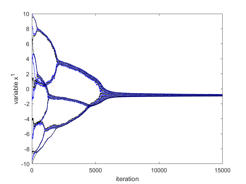
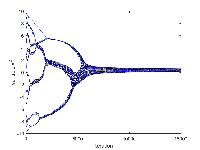
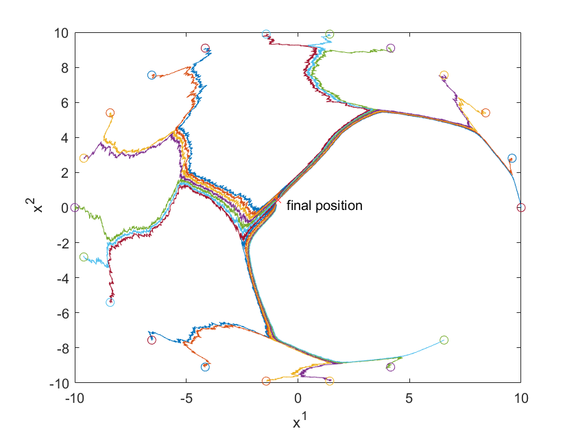
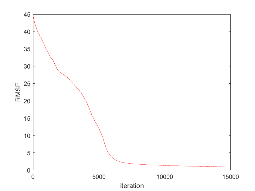
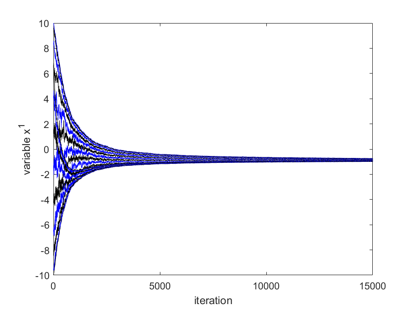
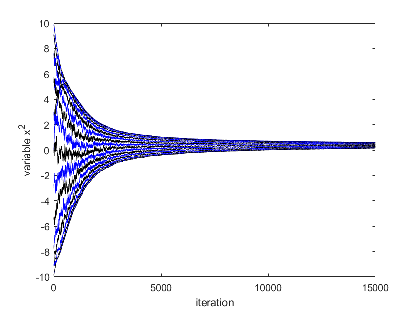
We use $\eta=0.8,\alpha_{t}=\frac{1}{1+t},t\geq 0,\beta=\frac{1}{K}=\dfrac{1}{1}$ for simulation. The initial position of agent $i$ is chosen to be $x_{i,0}=[10cos(\frac{(i-1)2\pi}{22}),10sin(\frac{(i-1)2\pi}{22})]^{T}$. The optimal solution of (13) in centralized way can be computed as mean of $d_{i},i=1,\ldots,20,$ and is $s^{*}=[-0.9002,0.4111]^{T}$. The results given by Algorithm (4.3) are shown in Figure 1-4. The error $e_{t}:=\|x_{t}-s^{*}\otimes\textbf{1}_{20}\|_{2}$, where $x_{t}=[x_{1,t}^{T},\ldots,x_{20,t}^{T}]^{T},$ is given in Fig. 4. The two-dimensional (2D) plot is shown in Figure 3. Figures 1-4 show that the positions of robotic agents are approaching the solution of the optimization (13) for one realization of random network with distribution dependency. Note that no existing result can solve this problem since the weights of links are both position-dependent and randomly arbitrarily activated.

We also simulate the above example with different weights than Cucker-Smale form, i.e.,

and the results are shown in Figures 5-6. The figures show that the variables of agents are getting consensus on the optimal solution of the problem.

Distributed optimization with both state-dependent interactions and random (arbitrary) networks is considered. It is shown that the state-dependent weighted random operator of the graph is quasi-nonexpansive; thus, it is not required to impose a priori distribution of random communication topologies on switching graphs. A more general optimization problem than that addressed in the literature is provided. A gradient-based discrete-time algorithm using diminishing step size is provided that is able to converge both almost surely and in mean square to the global solution of the optimization problem under suitable assumptions. Moreover, it reduces to a totally asynchronous algorithm for the distributed optimization problem. Relaxing strong convexity assumption of cost functions and/or doubly stochasticity assumption of communication graphs opens problems for future research.

References

- [1] Jakovetić, D., Bajović, D., Xavier, J., and Moura, J. M. F.: Primal-dual methods for large-scale and distributed convex optimization and data analysis. Proceedings of The IEEE. 108, 1923–1938 (2020)
- [2] Yang, T., Yi, X., Wu, J., Yuan, Y., Wu, D., Meng, Z., Hong, Y., Wang, H., Lin, Z., and Johansson, K. H.: A survey of distributed optimization. Annual Reviews in Control. 47, 278–305 (2019)
- [3] Mazlum, D. K., Dörfler, F., Sandberg, H., Low, S. H., Chakrabarti, S., Baldick, R., and Lavaei, J.: A survey of distributed optimization and control algorithms for electric power systems. IEEE Trans. on Smart Grid. 8, 2941–2962 (2017)
- [4] Nedić, A.: Distributed optimization. Encyclopedia of Systems and Control. 1–12 (2014)
- [5] Liberzon, D.: Switching in Systems and Control. Springer, New York (2003)
- [6] Cucker, F., and Smale, S.: Emergent behavior in flocks. IEEE Trans. Automatic Control. 52, 852–862 (2007)
- [7] Krause, U.: A discrete nonlinear and non-autonomous model of consensus formation. Communications in Difference Equations. Gordon and Breach, Amsterdam. 227–236 (2000)
- [8] Totsch, S., and Tadmor, E.: Heterophilious dynamics enhances consensus. SIAM Review. 56, 577-621 (2014)
- [9] Acemoglu, D., Ozdaglar, A., and Parandehgheibi, A.: Spread of (mis)information in social networks. Games and Economic Behavior. 70, 194–227 (2010)
- [10] Acemoglu, D., and Ozdaglar, A.: Opinion dynamics and learning in social networks. Dynamic Games and Applications. 1, 3–49 (2011)
- [11] Acemoglu, D., Como, G., Fagnani, F., and Ozdaglar, A.: Opinion fluctuations and disagreement in social networks. Mathematics of Operations Research. 38, 1–27 (2013)
- [12] Acemoglu, D., Bimpikis, K., and Ozdaglar, A.: Dynamics of information exchange in endogenous social networks. Theoretical Economics. 9, 41–97 (2014)
- [13] Heyselmann, R., and Krause, U.: Opinion dynamics and bounded confidence moels, analysis, and simulation. J. Artificial Societies and Social Simulation. 5, 1–33 (2002)
- [14] Blondel, V. D., Hendrickx, J. M., and Tsitsiklis, J. N.: On Krause’s multi-agent consensus model with state-dependent connectivity. IEEE Trans. on Autom. Contr. 54, 2586–2597 (2009)
- [15] Acemoglu, D., Ozdaglar, A., and Yildiz, E.: Diffusion of innovations in social networks. Proc. of 50th IEEE Conf. on Dec. Cont. and Europ. Cont. Conf., Dec. 12-15, Orlando, FL, USA. 2329–2334 (2011)
- [16] Simonetto, A., Kevicsky, T., and Babuška, R.: Constrained distributed algebraic connectivity maximization in robotic networks. Automatica. 49, 1348–1357 (2013)
- [17] Kim, Y., and Mesbahi, M.: On maximizing the second smallest eigenvalue of a state-dependent graph laplacian. IEEE Trans. on Autom. Contr. 51, 116–120 (2006)
- [18] Siljak, D. D.: Dynamic graphs. Nonlin. Analysis: Hybrid Syst. 2, 544–567 (2008)
- [19] Trianni, V., Simone, D. D., Reina, A., and Baronchelli, A.: Emergence of consensus in a multi-robot network: from abstract models to empirical validation. IEEE Robotics and Automation Letters. 1, 348–353 (2016)
- [20] Lobel, I., Ozdaglar, A., and Feiger, D.: Distributed multi-agent optimization with state-dependent communication. Math. Program. Ser. B. 129, 255–284 (2011)
- [21] Jing, G., Zheng, Y., and Wang, L.: Consensus of multiagent systems with distance-dependent communication networks. IEEE Trans. on Neural Networks and Learning Systems. 28, 2712–2726 (2017)
- [22] Jing, G., and Wang, L.: Finite time coordination under state-dependent communication graphs with inherent links. IEEE Trans. on Circuits and Systems-II: Express Briefs. 66, 968–972 (2019)
- [23] Shang, Y.: Constrained consensus in state-dependent directed multiagent networks. IEEE Trans. on Network Science and Engineering. 9, 4416–4425 (2022)
- [24] Sluc̆iak, O., and Rupp, M.: Consensus algorithm with state-dependent weights. IEEE Trans. Signal Processing. 64, 1972–1985 (2016)
- [25] Bogojeska, A., Mirchev, M., Mishkovski, I., and Kocarev, L.: Synchronization and consensus in state-dependent networks. IEEE Trans. on Circuits and Systems-I: Regular Papers. 61, 522–529 (2014)
- [26] Awad, A., Chapman, A., Schoof, E., Narang-Siddarth, A., and Mesbahi, M.: Time-scale separation on networks: consensus, tracking, and state-dependent interactions. IEEE 54th Annual Conf. on Decision and Control, Dec. 15-18, Osaka, Japan. 6172–6177 (2015)
- [27] Shi, G., Johansson, K. H., and Hong, Y.: Reaching an optimal consensus: dynamical systems that compute intersections of convex sets. IEEE Trans. Automatic Control. 58, 610–622 (2013)
- [28] Verma, A., Vasconcelos, M., Mitra, U., and Touri, B.: Maximal dissent: a state-dependent way to agree in distributed convex optimization. IEEE Trans. on Control of Network Systems. 10, 1783–1795 (2023)
- [29] Alaviani, S. Sh., and Elia, N.: Distributed convex optimization with state-dependent (social) interactions and time-varying topologies. IEEE Trans. Signal Processing. 69, 2611-2624 (2021)
- [30] Alaviani, S. Sh., and Elia, N.: Distributed multiagent convex optimization over random digraphs. IEEE Trans. Automatic Control. 65, 986–998 (2020)
- [31] Alaviani, S. Sh., and Kelkar, A. G.: Distributed convex optimization with state-dependent interactions over random networks. Proc. of IEEE Conf. on Decision and Control, Dec. 13-17, Austin, Texas, USA. 3149–3153 (2021)
- [32] Tsitsiklis, J. N.: Problems in decentralized decision making and computation. Ph.D. dissertation. Dep. Elect. Eng. Comp. Sci., MIT, Cambridge, MA (1984)
- [33] Bertsekas, D. P., and Tsitsiklis, J. N.: Parallel and Distributed Computation: Numerical Methods. Prentice Hall, Englewood Cliffs (1989)
- [34] Dotson, W. G.: Fixed points of quasi-nonexpansive mappings. J. Austral. Math. Soc. 13, 167–170 (1972)
- [35] Horn, R. A., and Johnson, C. R.: Matrix Analysis. Cambridge University Press, New York (1985)
- [36] Xu, H. K.: Iterative algorithms for nonlinear operators. J. London Math. Soc. 66, 240-256 (2002)
- [37] Alaviani, S. Sh., and Kelkar, A. G.: Asynchronous Algorithms for Distributed Consensus-Based Optimization and Distributed Resource Allocation over Random Networks. Proc. of Amer. Cont. Conf., June 8-10, Atlanta, GA, USA. 216–221 (2022)
- [38] Alaviani, S. Sh., and Elia, N.: Distributed average consensus over random networks. Proc. of Amer. Cont. Conf., July 10-12, Philadelphia, PA, USA,. 1854–1859 (2019)
- [39] Alaviani, S. Sh., and Elia, N.: A distributed algorithm for solving linear algebraic equations over random networks. IEEE Trans. on Automatic Control. 66, 2399–2406 (2021)
- [40] Kattepur, A., Rath, H. K., Mukherjee, A., and Simha, A.: Distributed optimization framework for Industry 4.0 automated warehouses. EAI Endorsed Transactions on Industrial Networks and Intelligent Systems. 5, 1–10 (2018)
- [41] Pahlavan, K., and Levesque, H.: Wireless Information Networks. Wiley, New York (1995)
- [42] Bubeck, S.: Convex optimization: algorithms and complexity. Foundations and Trends in Machine Learning. 8, 231–357 (2015)
- [43] Ryu, E. K., and Boyd, S.: A primer on monotone operator methods. Appl. Comput. Math. 15, 3–43 (2016)