Distributed Coverage Hole Prevention for
Visual Environmental Monitoring with Quadcopters
via Nonsmooth Control Barrier Functions
Abstract
This paper proposes a distributed coverage control strategy for quadcopters equipped with downward-facing cameras that prevents the appearance of unmonitored areas in between the quadcopters’ fields of view (FOVs). We derive a necessary and sufficient condition for eliminating any unsurveilled area that may arise in between the FOVs among a trio of quadcopters by utilizing a power diagram, i.e. a weighted Voronoi diagram defined by radii of FOVs. Because this condition can be described as logically combined constraints, we leverage nonsmooth control barrier functions (NCBFs) to prevent the appearance of unmonitored areas among a team’s FOV. We then investigate the symmetric properties of the proposed NCBFs to develop a distributed algorithm. The proposed algorithm can support the switching of the NCBFs caused by changes of the quadcopters composing trios. The existence of the control input satisfying NCBF conditions is analyzed by employing the characteristics of the power diagram. The proposed framework is synthesized with a coverage control law that maximizes the monitoring quality while reducing overlaps of FOVs. The proposed method is demonstrated in simulation and experiment.
Index Terms:
Control barrier functions, Multi-robot systems, Optimization and optimal control, Sensor networksI Introduction
Visual environmental monitoring has been utilized to collect information in a broad range of applications such as urban traffic [1], home/facility security [2], terrain data [3], and natural phenomena [4, 5]. Among the various types of robots utilized in these scenarios, unmanned aerial vehicles with visual sensors afford capturing vast environments from the sky. In addition, some unmanned aerial vehicles (e.g., quadcopters) are authorized to fly at relatively lower altitudes [6], which makes them suitable for capturing information at a closer distance to a surveilled area, which results in more detailed information. However, flying at a lower altitude typically leads to a smaller field of view (FOV) of the quadcopter, which in turn can make difficult to capture large-scale phenomena in vast environments.
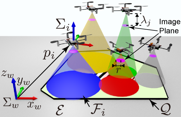
The restrictions associated with the FOV of a single quadcopter can be addressed by employing a team of quadcopters to cooperatively capture extensive environments. For instance, the research in [7] and [8] presents a surveillance system that can produce a single high-resolution panoramic video of a large target area in real-time by stitching together multiple videos from quadcopters. Furthermore, several empirical studies suggest that wider FOVs result in higher performance for human operators in human-robot interaction [9]. Thus, such collaborative monitoring systems could contribute to better situation awareness compared with receiving multiple disjoint videos provided individually by the quadcopters. However, the advantages provided by the joint monitoring efforts of a group of drones can be hindered by the potential appearance of unmonitored areas within the target environment, as illustrated in Fig. 1. Even though a quadcopter flies at a relatively lower altitude than conventional aerial vehicles, the altitude of quadcopters in environmental monitoring could exceed in some applications, e.g., [10]. In such cases, the size of the quadcopters’ FOVs becomes large, resulting in the appearance of a non-negligible unmonitored area between FOVs. Unmonitored areas are undesirable for situational awareness and search missions since they can lead to missing important events or failures when stitching videos together. Besides, such appearances of unmonitored areas among a team could result in overlooking potential hazards in safety-critical applications requiring real-time information, such as the monitoring of construction sites to prevent accidents [11].
This paper presents a coverage strategy for a team of quadcopters that prevents the appearance of unmonitored areas in-between FOVs of the quadcopters. We achieve this goal by modifying the nominal input maximizing the monitoring performance minimally invasive way so that the appearance of unmonitored areas is restricted. Specifically, we develop a distributed algorithm that employs nonsmooth control barrier functions (NCBFs), logically combined control barrier functions (CBFs), to prevent the appearance of a hole. Then, as the nominal input utilized with the algorithm, we propose the coverage control law that maximizes the monitoring performance of the team according to the perspective quality of the quadcopters’ cameras while expanding the surveyed area of a team by avoiding redundant observation of the multiple quadcopters.
I-A Related Work
Cooperative environmental monitoring has been studied extensively in the context of coverage control, which yields an optimal deployment of mobile sensors with respect to a spatial field in a distributed fashion [12, 13, 14]. The coverage control problem has been considered in a variety of scenarios, including networks of Pan-Tilt-Zoom (PTZ) cameras [15, 16, 17, 18] as well as teams of ground [19, 20, 21, 22] and aerial robots [23, 24, 25, 26].
In the context of aerial robots, the work in [23] presents a coverage strategy for a heterogeneous robot team where the cameras present various degrees of freedom depending on the robot type, e.g., PTZ cameras, quadcopters, etc. The proposed control law captures a 2D environment with a maximal resolution, where a better coverage quality is allocated to an area monitored by multiple cameras as opposed to the same area covered by a single camera. The work [24] proposes a solution that reduces FOV overlaps while guaranteeing the altitude of quadcopters within the predefined range. A more challenging scenario is considered in [25], where each quadcopter is mounted with a PTZ camera, making their FOVs become ellipses on the 2D environment. The work [26] presents the unified framework for both exploration and coverage problems in an unknown 3D environment with quadcopters. Both problems are formulated to maximize the portion of observed environments while minimizing the overlap of FOVs. Despite the variety of advances presented in these works, the proposed controllers do not address the appearance of unmonitored areas in between FOVs, which may result in overlooking critical events occurring in the environment.
The work in [27, 28] reduces the unmonitored area in the whole environment, rather than eliminating unobserved regions in-between FOVs, by maximizing the area of the covered region. Both works consider the agents with heterogeneous and fixed sensing regions. The uncovered areas are detected by utilizing a multiplicatively weighted Voronoi diagram having curved boundaries, where the weight of each sensor is equal to its sensing radius. The algorithms guarantee increased area coverage, but the elimination of unmonitored areas is not assured. The rejection of unmonitored regions is also considered in [29], where the total moving distance of mobile sensors is minimized. Still, this work assumes the sensing radius of all agents is fixed and identical. These methods, which assume a fixed or same measurement range, might not be readily extendable to cooperative monitoring with a team of quadcopters, where the size of FOVs dynamically evolves according to the changes of the zoom level or altitude. The work [30] proposes a solution based on a nonsmooth gradient flow for a disk-covering problem, where each agent can control its sensing radius. Because a disk-covering problem corresponds to completely covering the entire environment with disks of minimum radius, the proposed control law eliminates unobserved areas. The resulting final deployment renders the radius of sensing fields of all agents identical. However, it is difficult to cover the entire environment with high-resolution images in case the whole mission space is large compared with FOVs of quadcopters, or the number of quadcopters is limited. For instance, the monitoring area of [31] reaches . In such cases, rather than overextending FOVs for covering a whole area, preventing unmonitored areas around targeted regions under a team’s surveillance could yield more detailed information for contributing to the monitoring purposes. Furthermore, if the environment has non-uniform importance, allowing each quadcopter to decide on its sensing radius could lead to better monitoring performance because a team can adjust the resolution of the image according to the importance of the area. To achieve such a visual monitoring strategy, the team should maximize the objective function for visual monitoring quality, as in [23, 24, 25, 26]. However, in case the reduction or elimination of unmonitored areas is already encoded as the objective of the team as in [27, 28, 29, 30], the problem becomes a multi-objective optimization, with the associated challenges of balancing two different requirements.
In order to address the aforementioned issue, this paper prevents the appearance of a hole by means of a constraint-based approach, where the visual monitoring quality is maximized as long as unmonitored areas in-between a team are prevented. More specifically, the behavior of the quadcopters is constrained to prevent unsurveilled areas in-between quadcopters by CBFs. CBFs provide the forward invariance property to the admissible set of the robot state space [32, 33, 34]. CBFs have been employed in various applications ranging from bipedal robots [35, 36] to swarm robots [37, 38, 39, 40] and seeing success also in the context of environmental monitoring [41, 42, 43]. The work [41] proposes a control framework that guarantees the robot’s battery is never depleted during a monitoring task. Several charging models, such as solar lights and charging stations, are interpreted as a time-varying function defined in the mission space. Then, a time-varying CBF is developed to ensure energy constraints of the robots. The work [42] also utilizes the time-varying CBF to consider time-varying coverage control, where a density function specifying the importance of field changes dynamically. The proposed methods do not impose any requirements on the rate of change of the density functions and can be executed in a distributed fashion. In [43], a notion of information reliability is encoded through a time-varying density function as in [44], which decays if a region is not surveilled for a long period. Then, a patrolling motion is achieved by a time-varying CBF together with other safety constraints. In [45, 46], an extended version of CBFs are utilized to a quadcopter having nonlinear dynamics.
I-B Proposed Approach and Contributions
In this paper, we propose a control method that prevents unmonitored areas to arise in-between FOVs of quadcopters equipped with downward facing cameras while monitoring a mission area. First, CBFs preventing the appearance of unmonitored areas in between a team is designed by utilizing a power diagram. The power diagram [47] is a weighted Voronoi diagram defined by the different radii of FOVs, where the boundaries of the diagram are composed of lines known as the radical axis. We leverage this favorable property of the power diagram, compared with the multiplicatively weighted Voronoi partitions in [27, 28] that generate more complicated Voronoi cells composed of Appollonian circles, to analyze its feasibility and develop distributed algorithm. Furthermore, we provide the coverage control law that intends to monitor important regions while preventing too much overlap between the fields of view of quadcopters. The presented coverage controller is synthesized with the aforementioned CBFs to achieve the maximum visual monitoring quality while preventing the unmonitored areas in-between a team.
The contributions of this paper are as follows.
-
(a)
We develop a distributed algorithm preventing an unmonitored area in between a team of quadcopters based on CBFs. For this goal, the appearance of unsurveilled areas is encoded by the vertices of a power diagram. Because the derived constraints contain a Boolean logic, we leverage a nonsmooth control barrier function (NCBF) [48] to synthesize the controller that prevents an unmonitored area. We then formulate an algorithm that allows the jumps in the value of NCBF caused by the changes in the Delaunay graph induced by the power diagram.
-
(b)
We verify the feasibility of the proposed CBF-based methods. The existence of a control input that satisfies the constraints is closely related to how the CBF evolves together with the system dynamics. For example, in [49, 40], feasibility was established by showing that the gradient of the CBF does not vanish. In our case, this computation is not feasible and instead, we rely on the special structure of the power diagram to derive a simplified form of the designed CBFs’ derivatives. Then, we show that the set yielding the derivatives of CBF zero vectors can be neglected in practice. This result guarantees that the proposed CBF-based controller can generically generate the control input to prevent an unmonitored area in between a team during monitoring mission.
-
(c)
The coverage control law in our conference paper [50] is combined with the above CBF-based methods to showcase its utility. This visual coverage control serves two purposes: (i) improving the performance of the monitoring, considering the spatial sensing quality of cameras as in [17], and (ii) reducing the overlap between FOVs of the quadcopters to cover a large-scale area by a team.
-
(d)
The practical usefulness of the proposed monitoring strategy is demonstrated by simulations and experiments.
In our previous work [51], we proposed the preliminary results of (a), which does not allow a distributed computation without a strong assumption. More specifically, when the algorithm calculates the derivatives of CBFs for Quadcopter , it presumes the other quadcopters are fixed in the environment. In this paper, the algorithm is improved to achieve a distributed computation without the assumption by utilizing the symmetric properties of the proposed CBFs. We newly analyze the validity of the proposed NCBFs in (b), which was not discussed in our previous conference papers [51, 50]. The coverage control law discussed in (c) is proposed in our previous work [50], but we only show the utility of the control law with the preliminary algorithm that overly restricts a teams’s movement for preventing the appearance of unmonitored area in between quadcopters. Finally, this paper provides comprehensive simulation and experimental results demonstrating the effectiveness of the proposed methods.
II Preliminaries
In this section, we introduce several variations of CBFs, which can synthesize logically combined constraints in a system exhibiting graph changes. The methods will be needed to formulate the control algorithms preventing coverage holes in-between agents in Section IV.
Let us consider a control-affine system
| (1) |
where and are locally Lipschitz continuous while is measurable and locally bounded in both arguments. In this formulation, is not necessarily continuous. Therefore, the solution might not exist for the differential equation (1). To yield a system to which solutions exist, a system (1) can be turned into a differential inclusion via Filippov’s operator
| (2) |
with
| (3) |
where is a particular zero-Lebesgue-measure set and is an arbitrary zero-Lebesgue-measure set. As detailed in [52, 53], a Carathéodory solution, an absolutely continuous function such that almost everywhere on , always exists in the above system.
Hereafter, we introduce the CBF-based methods that confine the state of the system (2) in the admissible set. While the original papers [48, 53] assume a more general model than (2), we proceed with (2) as it is sufficient for our objective. In addition, we sometimes modify the notations in [48, 53] to suit our paper. Note that, in practice, the method introduced in this section does not require the computation of Filippov’s operator; instead, more convenient algorithm is formulated.
CBFs have been employed for guaranteeing the forward invariance property of the set , which represents constraints to be satisfied during the execution of the task. We assume that a set can be defined as the superlevel set of a barrier function , namely . Then, the forward invariance of the set can be accomplished by ensuring
| (4) |
for every Carathéodry solution, for some locally Lipschitz extended class- function [53].
Let us formulate the time-varying nature of (4) to better suit the problem we consider, where the constraints are added or subtracted according to the changes in the network graph of a team. First, the following two definitions are necessitated.
Definition 1.
Definition 2.
Definition 2 signifies the desirable behavior of the system. Namely, if the state is inside of the admissible set at the initial time and the state does not leave the set at any jump, then the state remains in the set. In the scenario introduced later on, the admissible set for Quadcopter switches every time its neighboring agents change. Therefore, by achieving the hybrid forward invariance of the set prohibiting the unsurveilled area in-between a team, the unmonitored area does not appear if the changes in the graph make no holes instantaneously. Furthermore, even if a change in the graph results in the appearance of a hole, such a hole can be eliminated by the general property of CBFs that yields the safe set attractive [53, 34]. This will be demonstrated in simulation in Section VI-C.
To capture the above requirements, we presume is not time-varying during each switching interval , which can be modeled with as
| (6) |
where the superlevel set of is denoted as .
In case is a zero-superlevel set of in (6), the properties of , especially its time derivative as appeared in (4) during , need to be investigated to guarantee the hybrid forward invariance of the set . Furthermore, if there exists nonsmoothness in the barrier function , e.g., as a result of logically combined constraints as in this paper, calculating can no longer be possible via the usual chain rule.
The barrier function embracing logically combined requirements is proposed in [48] as nonsmooth control barrier functions (NCBFs). The result of [48] revealed that the Boolean operations , , and are formulated as
| (7) |
at each . Let us assume that the NCBF described in (7) has the following favorable properties. Note that the definition from [48] has been modified to suit the terminology of this paper.
Definition 3.
[48, Definition 2] A locally Lipschitz function , where is an open and connected set, is a candidate NCBF if the set is nonempty.
Definition 4.
For ensuring the forward invariance of the set described by a smoothly composed candidate NCBFs, the work [48] introduces the almost-active set and the almost-active gradient.
Definition 5.
[48, Definition 7] Given and two candidate NCBFs , the almost-active set of functions for a candidate NCBF given by or is defined at each as
| (8) |
The almost-active gradient of an NCBF, denoted by , at a point is
| (9) |
The requirement (4) expressed with the almost-active gradient is integrated as a constraint in a quadratic programming (QP) problem to generate the control input guaranteeing the forward invariance of the set . If the formulated QP can always generate the control input, the designed NCBF is denoted as a valid NCBF as formally defined in the following theorem, where denotes a set-valued inner product.
Theorem 1.
Remark 1.
In practice, both the almost-active gradient and a set-valued inner product do not need to be evaluated in the QP. Instead, we can formulate constraints by including the gradients of all functions that constitute the index set defined in (8), eliminating the convex-hull operation as discussed in [53]. To see how this works, let us consider the system described as a single integrator, namely and , the same model we assume for quadcopters as will be introduced in (13). Then, instead of the QP in Theorem 1, we can employ
| (11a) | ||||
| (11b) | ||||
Similar to [48], let us assume that the resultant controller is measurable and locally bounded. Then, to guarantee the QP has a solution for every in the considered problem setting, namely the validness of the NCBF, we can investigate the following sufficient conditions: 1) is not an empty set, 2) , , . To consider the second condition, we analyze the gradients of the component CBFs of the designed NCBF in Section IV-C.
Having defined the validity of the NCBF necessitated to assure the forward invariance of , we are now ready to introduce the requirement for in (6). The following theorem formulates a valid hybrid NCBF (HNCBF), which is required to keep the safe set to be hybrid forward invariant.
Theorem 2.
Theorem 2 implies that we can render the set hybrid forward invariance by solving (11) at each switching sequence with valid NCBFs composing . In Section IV-C, following the above discussion, we analyze the validity of the proposed NCBF, namely the feasibility of the developed distributed algorithm. Please note that although the proposed algorithm utilizes NCBFs, a similar category of CBFs to [48, 53], the designed NCBF and its objectives are completely different from [48, 53]. Hence, analyzing the validity of the designed NCBFs necessitates new theoretical results, where we employ the properties of a weighted Voronoi partition. Furthermore, neither [48] nor [53] does not consider a distributed algorithm.
III Problem Statement
III-A Quadcopters and Environment
In this paper, we consider the scenario illustrated in Fig. 1, where quadcopters equipped with a downward facing camera are distributed in the 3-D space to monitor a 2-D region . We denote the region to be surveilled as the mission space hereafter, and assumed to be a closed and bounded convex subspace of the environment . The relative importance of points on is specified by a density function , where the higher the importance of a point is, the higher the value of , with . The goal of this paper is to monitor the important region while preventing the appearance of unmonitored areas in-between a team of quadcopters, shown as hatched areas in Fig. 1.
The world coordinate frame is placed so that its -plane is coplanar with the environment , where describes the standard basis of . Then, the set of coordinates of all points in the environment is defined as . We suppose that all quadcopters stay in the common half space during the operation.
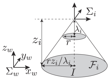
Let be the coordinate frame of Quadcopter , where its position vector with respect to is with , and its attitude is fixed to be consistent with that of regardless of the attitude of Quadcopter . We assume each quadcopter equips with a gimbal that can keep an optical axis of the camera corresponds with the axis of the -axis of . Namely, Quadcopter points its camera to the downward direction. In addition, each quadcopter is assumed to be equipped with localization devices, such as the GNSS, gyro sensors, and IMU, to estimate its own pose accurately, as in [54]. Let us express the image projection of the camera with a perspective projection model [55]. Then, the coordinate frame is located above the image plane with a distance the same as the focal length . We assume that all quadcopters have a circular image plane with radius . Then, Quadcopter can monitor all points inside of its field of view (FOV) described as
where its side view is illustrated in Fig. 2(a) with denoting Quadcopter ’s horizontal position projected on the environment .
The state of Quadcopter is denoted as , where the focal length specifies the zoom level of the camera. We assume that the dynamics of each quadcopter can be modeled as
| (13) |
which can be converted to reflect the dynamics of a quadcopter [56]. Note that higher-order dynamics could represent more aggressive motions, as in [45]. However, good quality images are typically paramount in environmental monitoring, which means quadcopters rarely fly with large accelerations, e.g., to prevent image blurs. Hence, we opt for first-order dynamics. Furthermore, this paper does not consider the disturbance, such as wind, assuming a controller implemented in each quadcopter can successfully cancel the effect as in [57].
III-B Communication Graph and Power Diagram
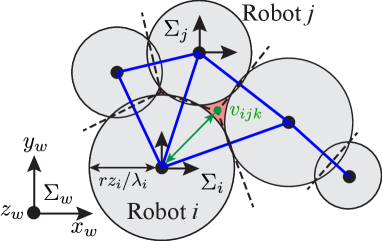
Every quadcopter is capable of sending its state to the neighboring quadcopters, where the inter-robot communication graph is modeled by the two undirected graphs and . First, is described as the graph which has an edge between the agents and if their FOVs are overlapped, namely . Second, is the graph generated by the power diagram, which is a form of the weighted Voronoi diagram, specified by the weighted distance
| (14) |
where in the second term signifies the radius of as shown in Fig. 2LABEL:sub@fig:test1. Hereafter, we call the distance (14) the power distance following [47]. Then, the communication graph is expressed as , which preserves the edges of power diagram only between those neighbors whose FOVs overlap, depicted by blue lines in Fig. 2LABEL:sub@fig:test2. The neighbors of Quadcopter in graph is denoted as .
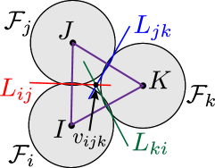
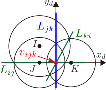
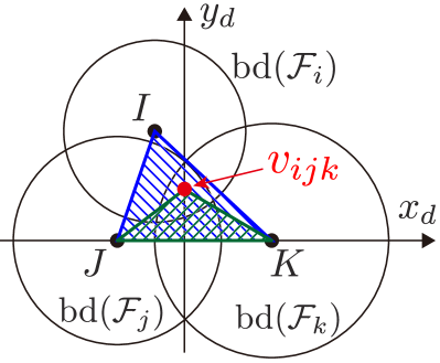
An example of a power diagram is shown in Fig. 3 with the graph . The bisector of two agents and is composed of a straight line known as the radical axis, along which both circles and , with the symbol to mean boundary of a set, have the same power distance. Namely, if we denote the radical axis between agent and as , holds. In addition, if with , then is satisfied. It is known that the radical axes defined by three circles whose centers are not collinear intersect in a common point termed the radical center, depicted with red dots in Fig. 3. The radical center is generated by three agents and forms a vertex of the weighted Voronoi cell with the weighted distance (14). Let us denote the radical center generated by , , and as . Then, from the property of the radical axis, the following condition is satisfied.
| (15) |
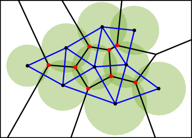
Since the graph is generated in a similar fashion to how the ordinary Voronoi diagram yields the Delaunay triangulation, the graph considered throughout this paper also provides triangular subgraphs as observed in Fig. 3. Let us denote the set of triangular subgraphs containing Quadcopter as its vertex as , where stands for triangular subgraphs111Although we should define a triangular subgraph of Quadcopter with , we use for notational simplicity.. Note that can be regarded as a subset of the Delaunay triangulation generated by the power diagram. Without loss of generality, we introduce the following assumption for a trio constituting a triangular subgraph .
Assumption 1.
No pair in , contains sensing regions that are concentric. In addition, no two axes among are parallel.
Under Assumption 1, the existence of the radical axes is assured, and all three axes intersect at a single point. Moreover, does not become a degenerate triangle, where denotes the triangle with vertices , , and . Note that becomes a degenerate triangle only when the pathological situation, and even if it happens, the proposed method can easily manage such an ill condition with a heuristic method, as shown in the simulation studies in Section VI-A.
Notice that the graph dynamically changes according to the quadcopters’ motion. We suppose that the set of triangular subgraphs does not change over intervals specified by a switching sequence as introduced in Definition 1.
The proposed scenario requires each quadcopter to exchange its state with the neighboring quadcopters. While one could consider employing a state estimation technique to obtain the neighbors’ state [58], the zoom level of the mounted camera, included in the state vector, is deemed challenging to estimate externally. Therefore, this paper presumes that each quadcopter is equipped with a communication device to send and receive its state. The communication devices and the challenges involved with outdoor communication, such as guaranteeing reliability by dedicating redundant networks and fail-safety, are detailed in [59].
III-C Unmonitored Areas to Be Prevented
Noticing that the power diagram generates convex cells, this paper prevents the formation of unmonitored areas in-between FOVs by including the Voronoi vertices , which exist in-between FOVs of teams, in each FOV, as shown in Fig. 3. Because each Voronoi vertex is generated by three agents except for degenerate Voronoi diagrams [60], we can separate the problem into triangular subgraphs . Note that this degeneracy does not cause serious problems because degenerate Voronoi diagrams can be divided into triangular subgraphs.
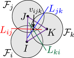
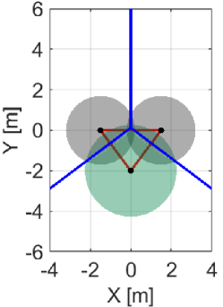
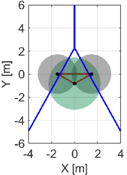
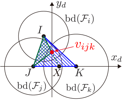
For the above reasons, we restrict our attention to the unmonitored regions that may appear among a trio determined by triangular subgraphs , illustrated in Fig. 4(a). This unsurveilled area is denoted as a hole hereafter and formally defined as follows.
Definition 6.
Consider a triangular subgraph , . A closed set is said to be a hole, if and only if it satisfies the conditions
| (16) | ||||
where denotes the interior of .
Since a hole in Definition 6 depends on a triangular subgraph that dynamically changes according to the switching sequence , the condition for preventing a hole also switches. Let us suppose that the zero superlevel set of a function with , , which we will derive in Section IV, describes the condition for Quadcopter to eliminate a hole in . By incorporating together, we obtain
| (17) |
the zero-superlevel set of which signifies the constraint Quadcopter must satisfy to prevent the formation in-between all triangular subgraphs . Then, the set
| (18) |
with HNCBF
| (19) | ||||
signifies the prevention of a hole is satisfied for Quadcopter during the entire mission.
The goal of this paper is to present a visual coverage framework that prevents the appearance of a hole by guaranteeing the hybrid forward invariance of the set . More specifically, during a monitoring task, we ensure no hole appears among FOVs of quadcopters if the changes of the graph do not make holes instantaneously in-between . Note that, in the proposed scenario, there is a possibility that changes of a graph yield a sudden appearance of a hole. For instance, as illustrated in the right part of Fig. 3, can have a dent. If the right-upper and right-lower quadcopters’ FOVs make overlap, a new subtrianglar graph is created. Although this graph change could alter the dent into a hole, the robustness of the forward invariance of the set can eliminate this suddenly appeared hole in most cases as will be shown in the simulation.
IV Prevention of Coverage Holes
In this section, we first derive the NCBF whose zero superlevel set encodes the prevention of a hole in during a time interval . Then, to prevent a formation of a hole, we develop a distributed algorithm that provides the hybrid forward invariance property of the set expressed as a superlevel set of HNCBF . Finally, we show that composing is a valid NCBF except for pathological points, hence the proposed algorithm can generically find the control input preventing a hole. In each procedure, we utilize the favorable properties of the power diagram incorporated in the designed CBFs.
IV-A Control Barrier Functions Preventing a Hole
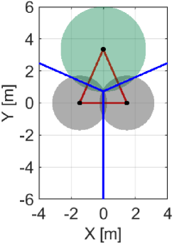
In this subsection, we formalize the condition to be satisfied for preventing a hole during a time interval . As discussed in Section III-C, an appearance of a hole in-between can be prevented by satisfying . However, as shown in Fig. 4(c), this condition is too conservative because certain movements of quadcopters are restricted, even if such movements do not form a hole. To alleviate this condition, let us consider the differences between Figs. 4(a) and (c), where a hole only appears in Fig. 4(a) although is outside of in either case. Then, we realize that, in Fig. 4(c), is outside of while the deployment in Fig. 4(a) is not. This observation leads us to introduce the following condition to prevent a formation of a hole
| (20) |
which requires Quadcopter to satisfy only when holds. The following theorem in our previous work [51] formalizes the relationship between (20) and the existence of a hole.
Theorem 3.
Let us consider Quadcopters , and , where each quadcopter’s FOV intersects with that of the other two quadcopters. Then, there is no hole in-between the three quadcopters if and only if the condition (20) is satisfied.
Proof.
See Theorem 1 in our conference work [51]. ∎

The condition appeared in (20) can be described as
| (21) |
where
| (22) |
is a candidate CBF satisfying if and only if and exist in the same half-plane separated by the line . Note that the denominator of (22) does not become under Assumption 1. By definition in (22),
| (23) |
holds for , where the same relationship is satisfied for and . The other condition in (20) is expressed with another CBF candidate as
| (24) |
The condition (20) preventing a hole in a triangular subgraph can be written as
| (25) |
From (7) and (25), the NCBFs of Quadcopter to be considered for preventing the formation of holes in-between all triangular subgraphs on the -th interval are described as
| (26) |
Here, we define , for each triangular subgraph , where they correspond with , , , and in order for notational simplicity.
IV-B Algorithm for Preventing a Hole
This subsection presents the distributed algorithm that prevents the appearance of a hole in-between a team even under the graph switches. Namely, the set in (18) defined with the HNCBF (19) and the NCBF (26) is rendered hybrid forward invariance by the algorithm. To calculate the control input in a distributed manner, we will utilize the symmetric property of the designed CBFs.
The hybrid forward invariance of the set can be guaranteed by satisfying the following constraint during each switching interval
| (27) |
for every Carathéodry solution, for some locally Lipschtz extended class- function [53]. However, the nonsmoothness exists in (26) hinders us from obtaining the time derivative via the usual chain rule.
As a remedy for this problem, we reformulate the constraint (27) by incorporating the gradients of all the functions comprising the almost-active set of functions as discussed in Remark 1. Then, the appearance of holes can be prevented by satisfying the following constraint on each interval
| (28) |
with the almost-active set of functions
| (29) | ||||
However, the input satisfying (28) cannot be calculated in a distributed manner because it requires input information of other agents . Furthermore, in order to evaluate the second term of the left side of (28), it requires the information of both and ; namely, neither Quadcopter nor can calculate it alone. The same issue occurs in the third term. The following theorem proves that condition (28) can be divided into three conditions, where each of them can be evaluated in a distributed manner by Quadcopters , , and , respectively.
Theorem 4.
Suppose that holes in the sense of Definition 6 do not appear in-between agents at the initial time of an interval , . Then, any measurable and locally bounded controllers , satisfying
| (30) | ||||
will render the safe set hybrid forward invariant.
Proof.
Let us consider the three agents . We show the condition (28) can be distributed in the form of the equation (30) from the symmetric property of the designed NCBF . First, from the equation (14) and (24), can be expressed by the power distance as
| (31) |
From the property of the power distance (15),
| (32) |
holds. Second, from (23), the NCBFs evaluating the condition takes the same value among . Hence, the synthesized NCBF (26) has the following symmetric property
| (33) |
Considering the fact that the derivatives of , , and take the same value among from (33), the condition (28) can be decomposed into
| (34a) | |||
| (34b) | |||
| (34c) | |||
This means that if each quadcopter satisfies the condition (30) , then the condition (28) is also satisfied. Notice that the inequalities (34b) and (34c) no longer contain either or the gradients of its components, hence Quadcopters and can evaluate (34b) and (34c) alone, respectively. This completes the proof. ∎
Theorem 4 signifies that each quadcopter can calculate the NCBF condition (30) in a distributed manner to render the admissible set hybrid forward invariant. More specifically, if the state trajectory does not leave the admissible set at the initial time of the switching interval , the formation of holes during each switching interval can be prevented by a control input satisfying the condition (30). Therefore, given a nominal control input for maximizing the monitoring performance, which will be presented in Section V, the QP modifying minimally invasive way to prevent the appearance of holes during each switching interval can be expressed as
| (35) |
where is the weighting matrix that adjusts the unit differences between and . The whole procedure is presented in Algorithm 1.
Remark 2.
The proposed algorithm assumes that each quadcopter can accurately estimate its position and attitude. Although the accuracy of the attitude estimation of the quadcopters generally has sufficient performance, e.g., around a few degrees in [61], the position estimation could contain an error depending on the estimation method, such as GNSS [62, 63]. If an upper bound of the estimation error is known a priori, one possible remedy to prevent holes even with estimation uncertainties could be to formulate a guaranteed FOV, the area guaranteed to be monitored by a quadcopter even with localization uncertainties, as presented in [25]. Because the guaranteed FOV constitutes the circular FOV, we can apply the proposed NCBFs to the power diagram based on the guaranteed FOV.
Remark 3.
If imperfect communication causes an error between the communicated and the actual state, one could employ the same approach as Remark 2 to deal with the error. If a communication edge is completely disconnected, a trio containing the disconnected edge faces difficulty calculating the NCBF. In such cases, a quadcopter could estimate the other quadcopters’ state while fixing the state that is difficult to estimate externally, e.g., a zoom level, to a predefined value.
Remark 4.
The proposed method considers the scenario where all quadcopters have a circular image plane. Considering other shapes of image planes would be worthwhile. However, other image shapes can pose challenges in formulating Voronoi partitions amenable to the NCBFs formulation. For instance, if we consider an elliptic image plane, a Voronoi partition generally becomes a complicated shape [64]. Still, as conducted in [20], by synchronizing the yaw-angle of the quadcopters, the Voronoi cell can be formulated as a convex polygon to which our proposed method can be extended.
IV-C Validity of the Proposed CBFs
As discussed in Section II, to show the validness of the HNCBF, we need to exhibit the validity of the proposed NCBFs. Since the individual gradients of the component functions in (25) at each point in time is smooth under Assumption 1, the designed NCBF is a smoothly composed candidate NCBF consisted by a Boolean operator in (7). Therefore, as a sufficient condition to guarantee the validity of the proposed NCBF, we investigate whether holds for each CBF (21), (22), and (24) composing NCBF as discussed in Remark 1.
In our previous works [50, 51], complexities appeared in the derivative of the radical center with respect to hinder us from analyzing the condition and elucidating the properties of each CBF’s derivative. To overcome this difficulty, we introduce a new coordinate frame on the environment , without loss of generality, that intends to simplify . Since we intend to derive , the circles and , namely and , are considered to have some constant values in this subsection. This corresponds with the fact that and are held constant when we calculate the partial derivative .
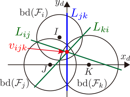
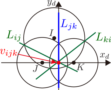
The coordinate frame on the environment is illustrated in Fig. 5. The introduced coordinate frame is arranged so that its -axis and -axis correspond with the line and the radical axis , respectively. In addition, we define the position vector of a point with respect to as , e.g., are denoted as after it is transformed from to the coordinate frame . Note that the value of partial derivatives calculated in differs from those derived in . However, as both and are fixed in the environment, the analysis in is enough to inspect whether holds and derives the condition otherwise.
Considering the fact that the radical center is always on the radical axis , the following condition is satisfied on the frame .
| (36) | |||
| (37) |
Futhermore, coincides with the -intercept of the radical axis , and derived as
| (38) |
with denoting the radius of . Note that from Assumption 1.
We are now ready to analyze the validness of each CBF. The following lemma investigates .
Lemma 1.
Proof.
See Appendix A. ∎
From (15) and (31), the condition derived in Lemma 1 must make the derivatives of and zero vectors too. Lemma 1 proves such a situation, in which the transitions of on do not influence the value of and , only happens when both the line and are orthogonal to the radical axis as shown in Fig. 6LABEL:sub@fig:diff_h_F. Nevertheless, the condition is generally non-stationary points, hence the state of Quadcopter does not keep satisfying such an ill condition. Hence, in practice, the condition induced from can generically yield a valid controller during a monitoring mission.
We next derive the following lemma that indicates is a valid CBF.
Lemma 2.
Suppose that Assumption 1, , and hold. Then, is a valid CBF when .
Proof.
See Appendix B. ∎
Finally, we investigate and .
Lemma 3.
Suppose that Assumption 1 and hold. Then, except for which makes the radical axis lie on the line , the function is a valid CBF when .
Proof.
See Appendix C. ∎
Since and are symmetric with respect to -axis, the following lemma immediately holds from Lemma 3.
Lemma 4.
Suppose that Assumption 1 and hold. Then, except for which makes the radical axis lie on the line , the function is a valid CBF when .
Fig. 6LABEL:sub@fig:diff_h_IJK illustrates the condition, where holds. Lemma 3 and 4 revealed that the derivatives of the proposed CBFs do not become zero vectors except for limited conditions. Similar to the discussion about , Quadcopter does not keep satisfying this condition. Therefore, the controller can render an input that satisfies the constraint incurred by and in practice.
From the discussion in this subsection, it is ensured that, except for a few pathological conditions, Algorithm 1 employing the QP (35) can find the control input preventing a hole in-between neighboring agents determined by triangular subgraphs . This results in the following theorem about the validity of the proposed NCBF.
Theorem 5.
Proof.
Theorem 5 guarantees that the QP (35) in each switching interval yields a control input preventing the appearance of a hole in most parts of its domain. Hence, from Theorem 2, the proposed distributed algorithm can render the set hybrid forward invariant except for the pathological conditions stated in Theorem 5. Note that Theorem 5 presumes holds. This corresponds with the fact that Quadcopter always has a trivial solution to eliminate a hole, where Quadcopter expands its FOV to cover other Quadcopters FOVs entirely. In summary, the proposed QP (35) has a feasible solution for preventing holes, except for a few limited conditions that do not cause severe issues in practice.
V Coverage Control
Having designed the control method that prevents the appearance of a hole in-between a team, we present the nominal control input in (35) that maximizes the monitoring quality. The proposed control input improves a coverage cost that simultaneously serves two objectives: (a) quantifying the performance of all the cameras, including the appropriate zoom level and distance from the ground and (b) reducing the overlaps of FOVs among a team.
The monitoring performance of a point can be quantified with the model proposed in [17],
| (39) |
with characterizing the perspective quality
and the loss of resolution
Note that the parameters signify the spatial resolution property of a camera, and models the desired distance to capture an environment. Note that renders a higher value as the focal length , namely the zoom level, increases, though the size of FOV becomes smaller. If a point is not in , then we set
The quality of coverage achieved by the team of quadcopters is characterized as
| (40) |
with and a density function , which achieves a higher value when the mission space is well monitored. By introducing the region allocated to Quadcopter according to the conic Voronoi diagram [17]
| (41) |
the cost in (40) can be rewritten as
| (42) |
However, the coverage cost (42) does not penalize the overlaps of FOVs, which might lead several quadcopters to monitor a same region. These overlaps of FOVs can deteriorate the monitoring performance since a team could potentially monitor a wider area by prompting those quadcopters to cover different areas. Let us define the region monitored by Quadcopter where another quadcopter in a team has a better sensing quality as
Then, the performance loss induced by the overlaps of FOVs is evaluated as
| (43) |
As we are interested in minimizing the overlap of FOVs evaluated in (43) while maximizing the coverage quality in (42), the overall objective can be encoded as
| (44) |
with the weight .
The nominal control input to maximize the objective function (44) can be obtained in a distributed manner by following a gradient-ascent method as
| (45) |
In our conference work [50], the gradient of is derived as
| (46) |
The following theorem in our conference paper [50] guarantees the convergence of the proposed coverage input .
Theorem 6.
Let Quadcopter , with state , evolve according to the control law , with
| (47) |
then, as , the team of quadcopters will converge to a critical point of the locational cost in (44).
Proof.
See Theorem 1 in our conference work [50]. ∎
Remark 5.
The computational complexity of the proposed control strategy can be calculated by evaluating the three processes involved: the computation of the power diagram, the QP optimization problem (35), and the coverage control input (47). First, the computational complexity of finding the Voronoi cell of Quadcopter in a distributed manner is known as , where stands for the number of neighbors Quadcopter has to consider. In the worst-case scenario, where Quadcopter ’s FOV is overlapped with all others’ FOVs, the computational complexity is . Second, the QP (35) can be solved by the interior point method, the computational complexity of which is , where stands for the dimension of the optimization variable. Since the optimization variable of the QP (35) is , (), its computational burden is low. Finally, the coverage control input is calculated by discretizing the integral in (47), similar to [23]. Its computational complexity depends on how many grids we utilize for a discretized approximation. In the current implementation, the computation time of (47) is around several milliseconds. More details on the computational complexity of calculating the Voronoi cell, the QP with CBF, and the coverage control law can be found in [65], [37], and [23], respectively.
VI Simulations and Experiments
VI-A Comparison between NCBF and CBF
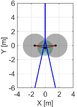
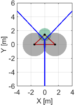
We first exemplify how the proposed NCBF prevents a hole while reducing too conservative behavior that appears in the case if we utilize alone, as discussed in Section IV-A. Minimizing how much the nominal controller, such as the coverage controller (45), is modified is crucial for optimizing the coverage performance because too conservative constraints hinder the controller from maximizing the coverage cost, resulting in a significant deterioration of the monitoring performance. Let us consider a team of three quadcopters composing , where the green Quadcopter moves upwards while the other two quadcopters stay in the initial positions, as shown in Fig. 7. The power diagram is depicted in blue, with in red. Note that the intersection of three boundaries corresponds with the radical center .
Fig. 7LABEL:sub@fig:sim_trio_Initial depicts the initial configuration of the three quadcopters. Figs. 7LABEL:sub@fig:sim_trio_NCBF1 and LABEL:sub@fig:sim_trio_NCBF2 show the simulation results with the proposed NCBF . Because allows the radical center to leave when as shown in Fig. 7LABEL:sub@fig:sim_trio_NCBF1, Quadcopter successfully passes through in-between two agents without being disturbed by . In contrast, since does not allow to leave , overly modifies the nominal input for Quadcopter even if the nominal input does not produce a hole. This overly modified input makes smaller so that Quadcopter can keep moving upwards while is inside of , though such modification is unnecessary to prevent a hole, as shown in Figs. 7LABEL:sub@fig:sim_trio_CBF1-LABEL:sub@fig:sim_trio_CBF3.
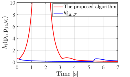
The evolution of and in each simulation is shown in Fig. 8. in the proposed method switches its value from to around 0.1s and back at 3.1s, accompanied by the nonsmooth transitions in Fig. 8. In contrast, if we utilize only , its value continues to keep a small value until s, resulting in too conservative modification of the nominal input.
Note that in the proposed algorithm takes a significantly large value from s to s. This peak is associated with the configuration of a team that makes a degenerate triangle, namely, the unsatisfaction of Assumption 1, which leads the denominator of (22) to a small value. Nevertheless, since the area of is close to zero and the radical center exists at infinity under such a degeneracy, the condition is satisfied. Therefore, we can regard that the team is still in the safe set defined as the zero-superlevel set of (26). Still, a too large value in the NCBF could cause a numerical error when we solve the QP. To circumvent this problem in the implementation, if one of is listed in and takes a significantly large value, we allow the QP not to evaluate the corresponding constraint because the team is deemed not to break the constraint in the next few steps.
VI-B Comparison to the previous work [51]
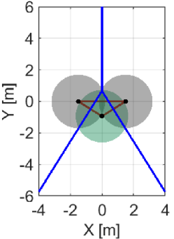
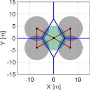
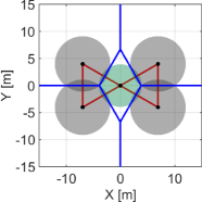
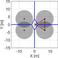
Let us next compare the proposed method with the authors’ previous work [51] to demonstrate Algorithm 1 can prevent the appearance of holes even in scenarios where the one in [51] cannot. Fig. 9LABEL:sub@fig:initial_comp shows the initial configuration of the five quadcopters composing two trios. The green Quadcopter has the nominal input decreasing its altitude with 3 m/s, while the other four quadcopters stay in the initial positions. The power diagram is depicted in blue, with each trio shown in red. The parameters are set as and , with the extended class- function .
The final configuration of the team with the proposed algorithm and the method in [51] are shown in Fig. 9LABEL:sub@fig:fin_comp_prop and Fig. 9LABEL:sub@fig:fin_comp_ICRA20, respectively. First, the proposed method successfully prevents the appearance of the holes by modifying the nominal input. The prevention of the holes can also be confirmed in Fig. 10, where each trio’s NCBF, shown in red and blue lines, keeps positive values. On the other hand, the method in [51] suffers from the oscillation of each NCBF, and both of the trios’ NCBF cannot remain positive, as depicted in violet and orange lines. After 3.1 s, the left trio is disconnected, as shown in Fig. 9LABEL:sub@fig:fin_comp_ICRA20, and only the right trio’s NCBF is evaluated. The simulation study demonstrates the proposed algorithm successfully prevents the appearance of holes even in scenarios where the method in [51] cannot.
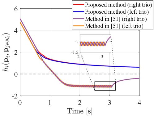
The main reason the method in [51] violates the constraint is that Quadcopter with the method in [51] only evaluates the minimum NCBF among all the trio it belongs to and the NCBFs in the range of from the minimum NCBF. Therefore, if the pre-determined is smaller than the quadcopters’ speed, the NCBF could be violated by showing chattering, as shown in Fig. 10. Algorithm 1 solves this issue by means of Theorem 4. Theorem 4 utilizes the symmetric property of the proposed NCBF to develop a constraint that each quadcopter can evaluate locally and shows that each quadcopter has to evaluate all the NCBFs of the trio that each quadcopter belongs, as shown in (35). Because of this theoretical guarantee and improvements in Algorithm 1, the proposed method successfully prevents holes.
VI-C Simulation with Nine Quadcopters
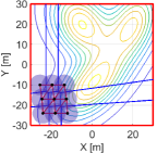
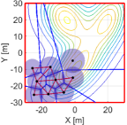
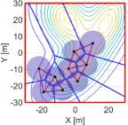
In the following simulation, the proposed algorithm is implemented with the coverage control law to the team of nine quadcopters. We then compare the algorithm with the nominal input in (45). The size of the mission space is , where the density function is depicted as the contour maps in Fig. 11. The parameters are set as , , , with the extended class- function .
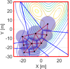
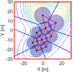
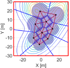
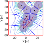
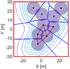
We then run the proposed algorithm from the initial configuration in Fig. 11LABEL:sub@fig:sim9_k1, where the red and blue lines show the triangular subgraphs in the graph and the power diagram, respectively. The snapshots of the simulation are depicted in Fig. 11. In the transition from Fig. 11LABEL:sub@fig:sim9_k1 to Fig. 11LABEL:sub@fig:sim9_k2100, we can confirm several triangular subgraphs in the team show switching, allowing them to move smoothly to the important region. At 4500 step, a team completely covers the peak of the density function in the lower part and continuously moves to cover two other peaks on the top part, as shown in Fig. 11LABEL:sub@fig:sim9_k4500. At the final configuration in Fig. 11LABEL:sub@fig:sim9_k10000, a team successfully covers three peaks with no hole.
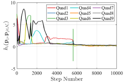
The evolution of HNCBFs is shown in Fig. 13, where all of them take the positive value except for the 5642 step. As discussed at the end of Section III-C, this sudden appearance of a hole is caused when a team closes a dent in the upper left part of Fig. 11LABEL:sub@fig:sim9_k4500. In other words, this instantaneous hole is caused by the inherent nature of the hybrid forward invariance [53] that does not address whether a system remains within the admissible set at the time switching occurs. Nevertheless, because of the robustness of the proposed algorithm, which stems from a general characteristic of CBFs yielding the admissible set attractive [53, 34], the proposed algorithm successfully eliminates this suddenly generated hole. Note that this formation of a hole does not violate the hybrid forward invariance of the set in Definition 2, as the concept presumes the state does not leave the safe set at each switching time .
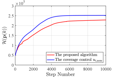
Fig. 12 shows the snapshots of the simulation results with the nominal input (45), where we set the same initial configuration to Fig. 11LABEL:sub@fig:sim9_k1. As shown in Fig. 12LABEL:sub@fig:sim9_cov_k500, from an early stage of the simulation, a team exhibits the unsurveilled area in-between quadcopters, which is developed from a hole created in-between a trio. In contrast, since a team does not need to consider an HNCBF constraint, a team moves a bit faster than the proposed method. As a result, quadcopters reach the configuration shown in Fig. 12LABEL:sub@fig:sim9_cov_k1800 at step, a similar configuration achieved by the proposed method at step. In return for this slightly fast transition, the unsurveilled area keeps appearing in a team, which might overlook the region even if the density function at the area takes a large value, roughly 80% of the highest peak of the density function, as shown in Fig. 12LABEL:sub@fig:sim9_cov_k6500. This hole keeps remaining until the end of the simulation shown in Fig. 12LABEL:sub@fig:sim9_cov_k10000. Fig. 14 shows the evolution of the coverage cost in (45), where the attained coverage cost of the proposed method is lower than that of the coverage controller because the proposed method modifies the nominal input to prevent the appearance of holes. However, as shown in Fig. 11LABEL:sub@fig:sim9_k10000, the proposed method successfully covers all three peaks of the density function without overlooking the important area in-between the team. This monitoring strategy prevents the overlooking of significant or safety-critical information in the monitoring mission.
VI-D Experimental Results with Five Quadcopters
This section demonstrates the proposed algorithm through experiments while comparing it with the results of the coverage control in (45). The size of the experimental field is . We implement the control law to a team of quadcopters composed of five Bitcraze Crazyflie 2.1 (), where their FOVs are virtually set. Each parameter is set as , , , , , with the extended class- function .
The schematic of the testbed is illustrated in Fig. 15, which consists of two desktop computers, a motion capture system (OptiTrack), and quadcopters. The motion capture system is composed of eleven PrimeX13 and the Windows PC installed with the tracking system Motive. This motion capture system captures the position of drones every ms and sends it to the Linux PC (Ubuntu 20.04). In the Linux PC, the Crazyswarm platform [66] allows us to receive the position information from the motion capture system. This information is sent to MATLAB to calculate the control input. Although the control architecture is implementable in a distributed manner, the current experimental system implements the proposed method in a Linux computer because of hardware limitations. Then, the calculated velocity input is sent to the drones through the Crazyswarm which manages a communication between the Linux PC and drones via the Crazyradio. The computation time of velocity input for five drones in MATLAB is roughly ms. Note that the control of attitude is conducted by the off-the-shelf controller implemented in the Crazyflies 2.1 so that it follows a reference velocity with ensuring a sufficient update rate of the attitude control.
We run the proposed algorithm from the initial configuration in Fig. 16LABEL:sub@fig:exp_HNCBF1, where Figs. 16LABEL:sub@fig:exp_HNCBF2-LABEL:sub@fig:exp_HNCBF5 show the snapshots of subsequent results. At s, two quadcopters near the peak of the density function move fast to the important area, as shown in Fig. 16LABEL:sub@fig:exp_HNCBF2. Although this transition makes the relative distance between each quadcopter larger, the appearance of a hole is prevented by expanding their FOVs. Then, at s in Fig. 16LABEL:sub@fig:exp_HNCBF3, a team reaches the important area followed by the configuration at s in Fig. 16LABEL:sub@fig:exp_HNCBF4, which allows a drone to capture the peak of the density at the center of FOV. Toward the final configuration shown in Fig. 16LABEL:sub@fig:exp_HNCBF5, two quadcopters on the bottom are going to combine their FOVs, resulting in a new edge in the graph.
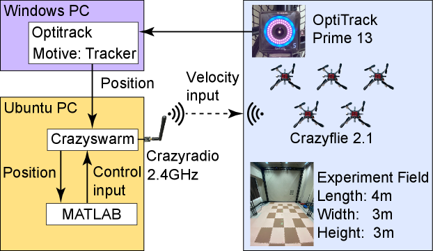
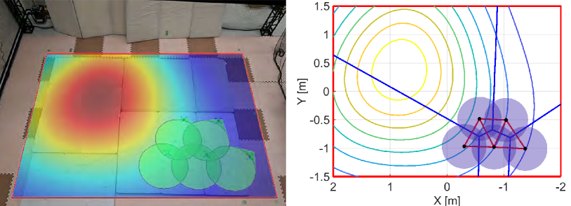
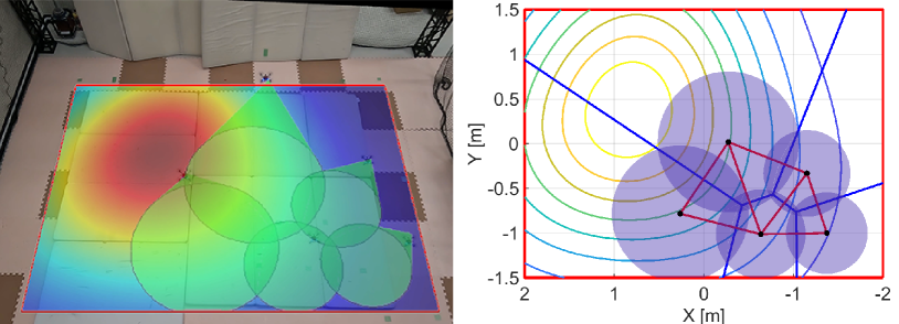
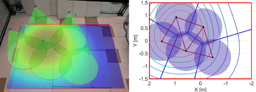
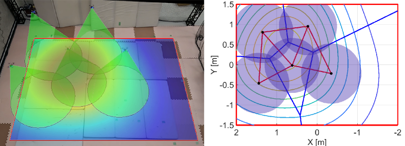
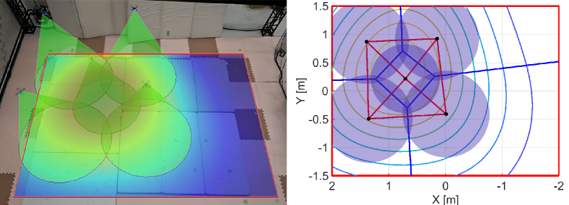
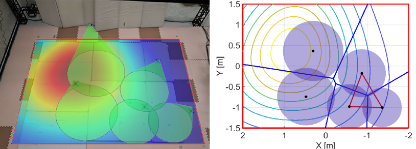
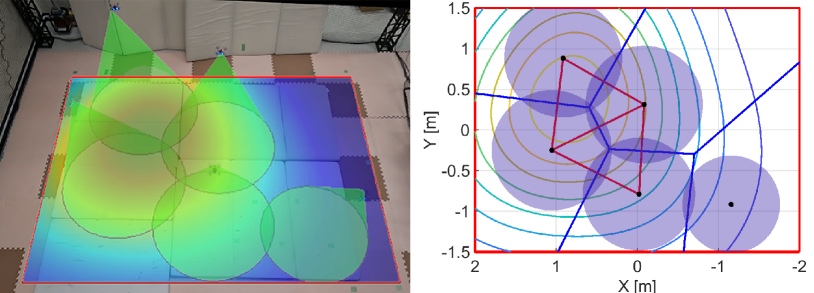
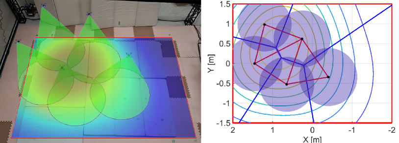
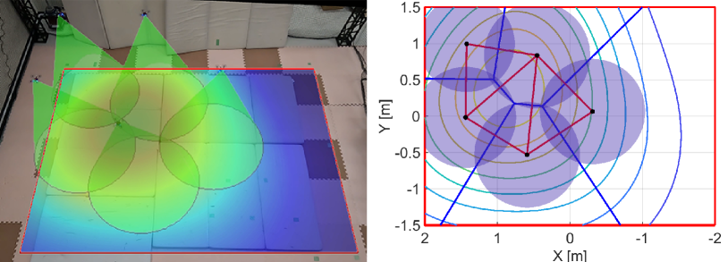
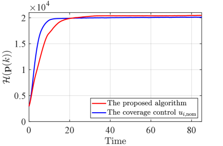
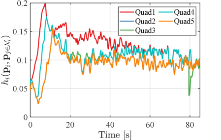
Fig. 17 shows the results with the nominal input only, where the initial configuration is the same as Fig. 16LABEL:sub@fig:exp_HNCBF1. We can confirm from Fig. 17LABEL:sub@fig:exp_nominal1 that a hole appears in the middle of the team at s. Fig. 17LABEL:sub@fig:exp_nominal2 shows the quadcopters located on the right do not preserve the triangular subgraph as opposed to the results with the proposed algorithm. The convergence speed is a bit shorter than that of the proposed method, and the quadcopters reach a peak of the density function at s as shown in Fig. 17LABEL:sub@fig:exp_nominal3. The team keeps the almost same configuration for the rest of the experiment while making small holes. The final configuration is shown in Fig. 17LABEL:sub@fig:exp_nominal4.
The evolution of the coverage cost (44) is shown in Fig. 18. The nominal input allows the team to achieve the maximum at s, while the proposed algorithm reaches the same value at s. Remarkably, even though the proposed algorithm modifies the nominal controller maximizing the coverage cost to prevent holes, the team attains the same coverage cost as the nominal coverage controller solely aimed at maximizing coverage cost. This result implies that the proposed algorithm does not overly restrict the behavior of the team. Furthermore, differently from the coverage control only, the proposed method keeps increasing the objective function gradually. The proposed method attains a larger maximum because its property to connect each FOV leads to the configuration where one of the drones captures the peak of the density function at the center of its FOV, as illustrated in Fig. 16LABEL:sub@fig:exp_HNCBF5. In contrast, a drone with the coverage control in (45) repels other agents’ FOVs to minimize their overlaps while trying to reach the most important area. This property might make a team get stuck into a deadlock before one of them captures the peak of the density function, as shown in Fig. 17LABEL:sub@fig:exp_nominal4. Fig. 19 shows the evolution of HNCBFs in the proposed method, where we observe that they keep positive values throughout the experiment. At s, there is a jump in the value of HNCBF, which is caused by the addition of the edge in the graph from the configuration in Fig. 16LABEL:sub@fig:exp_HNCBF4 to Fig. 16LABEL:sub@fig:exp_HNCBF5.
VII Conclusion
In this paper, we proposed a distributed coverage algorithm that prevents the formation of unsurveyed regions in-between FOVs of quadcopters. The necessary and sufficient condition for eliminating holes among trios of a team was introduced from the property of the power diagram. This condition, encoded with a Boolean composition, was then incorporated as NCBFs to design the algorithm guaranteeing the hybrid forward invariance of the set, preventing the appearance of holes. From the symmetric property of the designed NCBFs, the proposed algorithm can be implementable in a distributed fashion. We guaranteed that the proposed algorithm can find a control input preventing a hole, except for a few pathological conditions, by analyzing the derivatives of each CBF composing NCBFs. The proposed algorithm was synthesized with the coverage control law that improves monitoring quality while reducing the overlaps of FOVs. The effectiveness of the proposed method was demonstrated via simulations and experiments.
There are several challenges to explore in the future. First, the robustness of the proposed method in the presence of uncertainty should be investigated further to be able to deploy the algorithm in more challenging scenarios, including outdoor environments. Foreseeable challenges include uncertainty in the position estimation and in inter-robot communications, with possible remedies entailing considering a conservative monitoring strategy or preparing a redundant system to mitigate possible failures, as discussed in Remarks 2 and 3. Finally, the extension to the other shapes of FOVs needs to be further investigated.
Appendix A Proof of Lemma 1
Proof.
If holds, then there exists , which satisfies that . Although the discussion in this appendix presumes the coordinate frame , we will drop the superscript .
The derivative of with respect to is given by
| (48a) | ||||
| (48b) | ||||
| (48c) | ||||
| (48d) | ||||
with and . Since the equations (36) and (37) hold in the introduced coordinate frame , we can simplify (48) by substituting these conditions as
| (49a) | ||||
| (49b) | ||||
| (49c) | ||||
| (49d) | ||||
The partial derivatives of contained in (49) can be derived from as
| (50a) | ||||
| (50b) | ||||
| (50c) | ||||
| (50d) | ||||
where from Assumption 1. By combining (49) and (50) together, we obtain
| (51a) | ||||
| (51b) | ||||
| (51c) | ||||
| (51d) | ||||
The equations (51) reveal that never happens except for in , which means the radical center lies on the line . This completes the proof. ∎
Appendix B Proof of Lemma 2
Proof.
We will drop the superscript in this appendix though the discussion is provided in . Similar with in (22), takes positive value if and only if and exist in the same half-plane divided by the line , which is regarded as -axis in . Noticing that and share the side as in Fig. 20LABEL:sub@fig:JKv, the following equations hold with denoting the area of as .
| (52) |
where we substitute (38) to derive (52). Note that under Assumption 1. Then, we obtain
| (53a) | ||||
| (53b) | ||||
| (53c) | ||||
| (53d) | ||||
From (53), never occurs if . This completes the proof. ∎
Appendix C Proof of Lemma 3
Proof.
We will drop the superscript in this appendix. With the introduced coordinated system , let us denote the -intercept of the line as , as illustrated in Fig. 20LABEL:sub@fig:IJv. Then, from the fact ,
| (54) |
with
| (55) |
By substituting (55) into (54), we obtain
| (56) |
From (56),
| (57a) | ||||
| (57b) | ||||
| (57c) | ||||
| (57d) | ||||
hold. The equations (57) reveal that never happens except for the following condition is satisfied.
| (58) |
From (38), the left condition of (58) corresponds with . This signifies the radical axes and both pass through the origin. Since the right condition of (58) makes the line and the radical axis parallel, (58) is satisfied if and only if lies on the line . This completes the proof. ∎
References
- [1] H. Zhou, H. Kong, L. Wei, D. Creighton, and S. Nahavandi, “Efficient road detection and tracking for unmanned aerial vehicle,” IEEE Trans. Intell. Transportation Syst., vol. 16, no. 1, pp. 297–309, 2015.
- [2] S. Fleck and W. Strasser, “Smart camera based monitoring system and its application to assisted living,” Proc. IEEE, vol. 96, no. 10, pp. 1698–1714, 2008.
- [3] D. T. Cole, A. H. Goktogan, P. Thompson, and S. Sukkarieh, “Mapping and tracking,” IEEE Robot. Automat. Mag., vol. 16, no. 2, pp. 22–34, 2009.
- [4] G. Zhou, C. Li, and P. Cheng, “Unmanned aerial vehicle (UAV) real-time video registration for forest fire monitoring,” in Proc. IEEE Int. Geoscience and Remote Sensing Symp., vol. 3, 2005, pp. 1803–1806.
- [5] M. Erdelj, E. Natalizio, K. R. Chowdhury, and I. F. Akyildiz, “Help from the sky: Leveraging UAVs for disaster management,” IEEE Pervasive Computing, vol. 16, no. 1, pp. 24–32, 2017.
- [6] H. Shakhatreh, A. H. Sawalmeh, A. Al-Fuqaha, Z. Dou, E. Almaita, I. Khalil, N. S. Othman, A. Khreishah, and M. Guizani, “Unmanned aerial vehicles (UAVs): A survey on civil applications and key research challenges,” IEEE Access, vol. 7, pp. 48 572–48 634, 2019.
- [7] X. Meng, W. Wang, and B. Leong, “Skystitch: A cooperative multi-UAV-based real-time video surveillance system with stitching,” in Proc. 23rd ACM Int. Conf. Multimedia, 2015, pp. 261–270.
- [8] J. J. Ruiz, F. Caballero, and L. Merino, “MGRAPH: A multigraph homography method to generate incremental mosaics in real-time from UAV swarms,” IEEE Robot. Automat. Lett., vol. 3, no. 4, pp. 2838–2845, 2018.
- [9] M. S. Prewett, R. C. Johnson, K. N. Saboe, L. R. Elliott, and M. D. Coovert, “Managing workload in humanârobot interaction: A review of empirical studies,” Computers in Human Behavior, vol. 26, no. 5, pp. 840–856, 2010.
- [10] M. A. Boon, A. P. Drijfhout, and S. Tesfamichael, “Comparison of a fixed-wing and multi-rotor UAV for environmental mapping applications: A case study,” Int. Arch. Photogrammetry, Remote Sensing and Spatial Information Sciences, vol. XLII-2/W6, pp. 47–54, 2017.
- [11] Y. Ham, K. K. Han, J. J. Lin, and M. Golparvar-Fard, “Visual monitoring of civil infrastructure systems via camera-equipped unmanned aerial vehicles (UAVs): A review of related works,” Visual. Eng., vol. 4, no. 1, 2016.
- [12] J. Cortes, S. Martinez, T. Karatas, and F. Bullo, “Coverage control for mobile sensing networks,” IEEE Trans. Robot. Automat., vol. 20, no. 2, pp. 243–255, 2004.
- [13] C. G. Cassandras and W. Li, “Sensor networks and cooperative control,” Eur. J. Control, vol. 11, no. 4, pp. 436–463, 2005.
- [14] S. Martinez, J. Cortes, and F. Bullo, “Motion coordination with distributed information,” IEEE Control Syst. Mag., vol. 27, no. 4, pp. 75–88, 2007.
- [15] C. Ding, B. Song, A. Morye, J. A. Farrell, and A. K. Roy-Chowdhury, “Collaborative sensing in a distributed PTZ camera network,” IEEE Trans. Image Processing, vol. 21, no. 7, pp. 3282–3295, 2012.
- [16] M. Forstenhaeusler, R. Funada, T. Hatanaka, and M. Fujita, “Experimental study of gradient-based visual coverage control on SO(3) toward moving object/human monitoring,” in Proc. Amer. Control Conf., 2015, pp. 2125–2130.
- [17] O. Arslan, H. Min, and D. E. Koditschek, “Voronoi-based coverage control of Pan/Tilt/Zoom camera networks,” in Proc. IEEE Int. Conf. Robot. Automat., 2018, pp. 1–8.
- [18] T. Hatanaka, R. Funada, and M. Fujita, “Visual surveillance of human activities via gradient-based coverage control on matrix manifolds,” IEEE Trans. Control Syst. Technol., vol. 28, no. 6, pp. 2220–2234, 2020.
- [19] K. Laventall and J. Cortes, “Coverage control by robotic networks with limited-range anisotropic sensory,” in Proc. Amer. Control Conf., 2008, pp. 2666–2671.
- [20] A. Gusrialdi, T. Hatanaka, and M. Fujita, “Coverage control for mobile networks with limited-range anisotropic sensors,” in Proc. 47th IEEE Conf. Decis. Control, 2008, pp. 4263–4268.
- [21] D. Panagou, D. M. StipanoviÄ, and P. G. Voulgaris, “Dynamic coverage control in unicycle multi-robot networks under anisotropic sensing,” Front. Robot. AI, vol. 2, no. 3, 2015.
- [22] J. Chen and P. Dames, “Distributed multi-target tracking for heterogeneous mobile sensing networks with limited field of views,” in Proc. IEEE Int. Conf. Robot. Automat., 2021, pp. 9058–9064.
- [23] M. Schwager, B. J. Julian, M. Angermann, and D. Rus, “Eyes in the sky: Decentralized control for the deployment of robotic camera networks,” Proc. IEEE, vol. 99, no. 9, pp. 1541–1561, 2011.
- [24] S. Papatheodorou, A. Tzes, and Y. Stergiopoulos, “Collaborative visual area coverage,” Robot. Autonomous Syst., vol. 92, pp. 126–138, 2017.
- [25] N. Bousias, S. Papatheodorou, M. Tzes, and A. Tzes, “Collaborative visual area coverage using aerial agents equipped with PTZ-cameras under localization uncertainty,” in Proc. Eur. Control Conf., 2019, pp. 1079–1084.
- [26] A. Renzaglia, J. Dibangoye, V. L. Doze, and O. Simonin, “A common optimization framework for multi-robot exploration and coverage in 3D environments,” J. Intell. Robotic Syst., vol. 100, pp. 1453–1468, 2020.
- [27] H. Mahboubi, K. Moezzi, A. G. Aghdam, and K. Sayrafian-Pour, “Distributed deployment algorithms for efficient coverage in a network of mobile sensors with nonidentical sensing capabilities,” IEEE Trans. Vehicular Technol., vol. 63, no. 8, pp. 3998–4016, 2014.
- [28] H. Mahboubi and A. G. Aghdam, “Distributed deployment algorithms for coverage improvement in a network of wireless mobile sensors: Relocation by virtual force,” IEEE Trans. Control of Network Syst., vol. 4, no. 4, pp. 736–748, 2017.
- [29] C. So-In, T. Nguyen, and N. Nguyen, “An efficient coverage hole-healing algorithm for area-coverage improvements in mobile sensor networks,” Peer-To-Peer Networking and Appl., vol. 12, no. 3, pp. 541–552, 2019.
- [30] J. Cortes and F. Bullo, “Coordination and geometric optimization via distributed dynamical systems,” SIAM J. Control Optim., vol. 44, no. 5, pp. 1543–1574, 2005.
- [31] K. Shah, G. Ballard, A. Schmidt, and M. Schwager, “Multidrone aerial surveys of penguin colonies in Antarctica,” Science Robotics, vol. 5, no. 47, p. eabc3000, 2020.
- [32] M. Egerstedt, Robot Ecology: Constraint-Based Design for Long-Duration Autonomy. Princeton University Press, 2021.
- [33] A. D. Ames, X. Xu, J. W. Grizzle, and P. Tabuada, “Control barrier function based quadratic programs for safety critical systems,” IEEE Trans. Autom. Control, vol. 62, no. 8, pp. 3861–3876, 2017.
- [34] A. D. Ames, S. Coogan, M. Egerstedt, G. Notomista, K. Sreenath, and P. Tabuada, “Control barrier functions: Theory and applications,” in Proc. Eur. Control Conf., 2019, pp. 3420–3431.
- [35] Q. Nguyen, A. Hereid, J. W. Grizzle, A. D. Ames, and K. Sreenath, “3D dynamic walking on stepping stones with control barrier functions,” in Proc. IEEE 55th Conf. Decis. Control, 2016, pp. 827–834.
- [36] M. Ahmadi, X. Xiong, and A. D. Ames, “Risk-averse control via CVaR barrier functions: Application to bipedal robot locomotion,” IEEE Control Syst. Lett., vol. 6, pp. 878–883, 2022.
- [37] L. Wang, A. D. Ames, and M. Egerstedt, “Safety barrier certificates for collisions-free multirobot systems,” IEEE Trans. Robot., vol. 33, no. 3, pp. 661–674, 2017.
- [38] R. Funada, X. Cai, G. Notomista, M. W. S. Atman, J. Yamauchi, M. Fujita, and M. Egerstedt, “Coordination of robot teams over long distances: From Georgia Tech to Tokyo Tech and back-An 11,000-km multirobot experiment,” IEEE Control Syst. Mag., vol. 40, no. 4, pp. 53–79, 2020.
- [39] M. Srinivasan, M. Abate, G. Nilsson, and S. Coogan, “Extent-compatible control barrier functions,” Syst. Control Lett., vol. 150, p. 104895, 2021.
- [40] K. Nishimoto, R. Funada, T. Ibuki, and M. Sampei, “Collision avoidance for elliptical agents with control barrier function utilizing supporting lines,” in Proc. Amer. Control Conf., 2022, pp. 5147–5153.
- [41] G. Notomista and M. Egerstedt, “Persistification of robotic tasks,” IEEE Trans. Control Syst. Technol., vol. 29, no. 2, pp. 756–767, 2021.
- [42] M. Santos, S. Mayya, G. Notomista, and M. Egerstedt, “Decentralized minimum-energy coverage control for time-varying density functions,” in Proc. Int. Symp. Multi-Robot Multi-Agent Syst., 2019, pp. 155–161.
- [43] H. Dan, T. Hatanaka, J. Yamauchi, T. Shimizu, and M. Fujita, “Persistent object search and surveillance control with safety certificates for drone networks based on control barrier functions,” Front. Robot. AI, vol. 8, p. 740460, 2021.
- [44] N. Hübel, S. Hirche, A. Gusrialdi, T. Hatanaka, M. Fujita, and O. Sawodny, “Coverage control with information decay in dynamic environments,” IFAC Proc. Volumes, vol. 41, no. 2, pp. 4180–4185, 2008.
- [45] G. Wu and K. Sreenath, “Safety-critical control of a planar quadrotor,” in Proc. Amer. Control Conf., 2016, pp. 2252–2258.
- [46] L. Wang, A. D. Ames, and M. Egerstedt, “Safe certificate-based maneuvers for teams of quadrotors using differential flatness,” in Proc. IEEE Int. Conf. Robot. Automat., 2017, pp. 3293–3298.
- [47] F. Aurenhammer, “Power diagrams: Properties, algorithms and applications,” SIAM J. Computing, vol. 16, no. 1, pp. 78–96, 1987.
- [48] P. Glotfelter, J. Cortés, and M. Egerstedt, “Boolean composability of constraints and control synthesis for multi-robot systems via nonsmooth control barrier functions,” in Proc. IEEE Conf. Control Technol. Appl., 2018, pp. 897–902.
- [49] G. Notomista, S. F. Ruf, and M. Egerstedt, “Persistification of robotic tasks using control barrier functions,” IEEE Robot. Automat. Lett., vol. 3, no. 2, pp. 758–763, 2018.
- [50] R. Funada, M. Santos, J. Yamauchi, T. Hatanaka, M. Fujita, and M. Egerstedt, “Visual coverage control for teams of quadcopters via control barrier functions,” in Proc. IEEE Int. Conf. Robot. Automat., 2019, pp. 3010–3016.
- [51] R. Funada, M. Santos, T. Gencho, J. Yamauchi, M. Fujita, and M. Egerstedt, “Visual coverage maintenance for quadcopters using nonsmooth barrier functions,” in Proc. IEEE Int. Conf. Robot. Automat., 2020, pp. 3255–3261.
- [52] J. Cortes, “Discontinuous dynamical systems,” IEEE Control Syst. Mag., vol. 28, no. 3, pp. 36–73, 2008.
- [53] P. Glotfelter, I. Buckley, and M. Egerstedt, “Hybrid nonsmooth barrier functions with applications to provably safe and composable collision avoidance for robotic systems,” IEEE Robot. Automat. Lett., vol. 4, no. 2, pp. 1303–1310, 2019.
- [54] P. Marantos, Y. Koveos, and K. J. Kyriakopoulos, “UAV state estimation using adaptive complementary filters,” IEEE Trans. Control Syst. Technology, vol. 24, no. 4, pp. 1214–1226, 2016.
- [55] Y. Ma, S. Soatto, J. Kosecka, and S. Sastry, An Invitation to 3-D Vision: From Images to Geometric Models. Springer-Verlag, 2003.
- [56] D. Mellinger and V. Kumar, “Minimum snap trajectory generation and control for quadrotors,” in Proc. IEEE Int. Conf. Robot. Automat., 2011, pp. 2520–2525.
- [57] B. Xiao and S. Yin, “A new disturbance attenuation control scheme for quadrotor unmanned aerial vehicles,” IEEE Trans. Industrial Informatics, vol. 13, no. 6, pp. 2922–2932, 2017.
- [58] A. R. Vetrella, G. Fasano, and D. Accardo, “Attitude estimation for cooperating UAVs based on tight integration of GNSS and vision measurements,” Aerospace Science and Technology, vol. 84, pp. 966–979, 2019.
- [59] S. Hayat, E. Yanmaz, and R. Muzaffar, “Survey on unmanned aerial vehicle networks for civil applications: A communications viewpoint,” IEEE Comm. Surveys and Tutorials, vol. 18, no. 4, pp. 2624–2661, 2016.
- [60] A. Okabe, B. Boots, K. Sugihara, and S. N. Chiu, Spatial Tessellations: Concepts and Applications of Voronoi Diagrams, Second Edition. Wiley-Blackwell, May 2000.
- [61] F. Hoffmann, N. Goddemeier, and T. Bertram, “Attitude estimation and control of a quadrocopter,” in Proc. IEEE/RSJ Int. Conf. Intell. Robots and Syst., 2010, pp. 1072–1077.
- [62] G. Balamurugan, J. Valarmathi, and V. P. S. Naidu, “Survey on UAV navigation in GPS denied environments,” in Proc. Int. Conf. Signal Processing, Comm., Power and Embedded Syst., 2016, pp. 198–204.
- [63] B. B. Ready and C. N. Taylor, “Improving accuracy of MAV pose estimation using visual odometry,” in Proc. Amer. Control Conf., 2007, pp. 3721–3726.
- [64] I. Z. Emiris and G. M. Tzoumas, “A real-time and exact implementation of the predicates for the Voronoi diagram of parametric ellipses,” in Proc. ACM Symp. Solid and Physical Modeling, 2007, pp. 133–142.
- [65] C. He, Z. Feng, and Z. Ren, “Distributed algorithm for Voronoi partition of wireless sensor networks with a limited sensing range,” Sensors, vol. 18, no. 2, p. 446, 2018.
- [66] J. A. Preiss, W. Hönig, G. S. Sukhatme, and N. Ayanian, “Crazyswarm: A large nano-quadcopter swarm,” in Proc. IEEE Int. Conf. Robot. Automat., 2017, pp. 3299–3304.