Distributed entanglement generation from asynchronously excited qubits
Abstract
The generation of GHZ states calls for simultaneous excitation of multiple qubits. The peculiarity of such states is reflected in their nonzero distributed entanglement which is not contained in other entangled states. We study the optimal way to excite three superconducting qubits through a common cavity resonator in a circuit such that the generation of distributed entanglement among them could be obtained at the highest degree in a time-controllable way. A non-negative measure quantifying this entanglement is derived as a time function of the quadripartite system evolution. We find that this measure does not stay static but obtains the same maximum periodically. When the qubit-resonator couplings are allowed to vary, its peak value is enhanced monotonically by increasing the greatest coupling strength to one of the qubits. The period of its peak to peak revival maximizes when the couplings become inhomogeneous, thus qubit excitation becoming asynchronous, at a relative ratio of 0.35. The study demonstrates the role of asynchronous excitations for time-controlling multi-qubit systems, in particular in extending entanglement time.
I Introduction
GHZ state is used ubiquitously in quantum crytography [1], quantum communication [2], and metrology [3]. Its generation among three qubits call for the distributed entanglement among all qubits [4] instead of the individual entanglements [5] between one qubit and the other two combined. Generalizing the scenarios to four or more qubits, the distributed entanglement is formally distinguished from the individual entanglements in terms of the monogamy relations [6, 7, 8]. The former is regarded as the difference between the group entanglement (one qubit entangles with all the others as a whole) and the sum of the monogamous entanglements (one qubit entangles with one other qubit). For an -qubit system, the difference is computed through a metric called polynomial invariant [9] for its invariance under local unitary transformations [10]. It extends the concept of concurrence [11, 12] and generalized the 3-tangle measure for tripartite systems [4, 13, 14, 15]. There are also proposals to measure -qubit entanglement through entanglement formation [16, 17].
Despite these extensive studies, they are commonly restricted to static entangled states. The question regarding entanglement dynamics is less well understood. Using information theoretic measure like distance function [18] or concurrence [19], the onset of entanglement accumulation can be found and distinct time behavior of entanglement evolution can be determined by system parameters such as coupling strengths for cavity-coupled qubits [20]. More recent studies investigate how entanglement can be protected from the effects of non-Markovian environments through time [3, 21, 22]. Despite these studies, how entanglement are distributed dynamically among multiple qubits in a unified system, making distinction between group entanglement and monogamous entanglement has, to our best knowledge, not yet been answered.
Here, we study an experimentally accessible circuit quantum electrodynamic (cQED) system [23, 24] comprising three superconducting qubits that are commonly coupled to one cavity bus, aiming to clarify the relationship between the coupling combinations and the temporal behavior of distributed entanglement. Specifically, we investigate how multiple qubits undergoing asynchronous excitation by uneven couplings would facilitate or deteriorate the generation of distributed entanglement. The deformed algebra technique [25, 26], which was used to study a similar quadripartite system for static entanglement analysis [27], is extended to the dynamic analysis. In addition, to accomodate the quadripartite system, we generalize the 3-tangle definition while specifying the polynomial invariant definition to introduce a 4-tangle measure to quantify the distributed entanglement that occurs in our cQED system. Numerically solving the equations of motion leads to a cyclic revival pattern of the 4-tangle, which are similar to the evolution dynamics of various qubit and cavity systems [28, 29, 30, 19].
More importantly, the individual qubit-cavity coupling strengths are varied and the resulting maximal 4-tangle and period of revival are statistically binned to find the optimal coupling strengths. We find that when the 4-tangle under all circumstances are periodically returned to zero to ensure the monogamous equality bound, the peak magnitude of obtainable 4-tangle increases monotonically with the absolute coupling strength if the couplings among the qubits are set uniform. This observation provides a positive correlation between monogamy and coupling strength. Moreover, the length of the period depends nonlinearly on the relative strength, i.e the ratio of the center qubit coupling to the side qubit coupling. In particular, statistical analysis shows that the period maximizes when the relative strength equals , showing that the inhomogeneity of coupling (thus asynchronous excitations to the qubits) in this case positively affects the generation of entanglement.
Environmental induced decoherences are omitted in our study to simplify the expressions for the state evolutions and the computation of the 4-tangle. This omission is experimentally justified because typical superconducting transmon qubits fabricated under current technologies have and relaxation times reach the order of 10s and sometimes even s [31]. In contrast, the characteristic times studied here for entanglement generation, such as the period of revival, is less than 1s. Therefore, the observations from the theoretical study is not affected by the finite coherence times. In the following, we present the model of the quadripartite system in Sec. II and define the measure of 4-tangle in Sec. III. The discussion relevant to the periodicity appearing in the monogamy inequality is presented in Sec. IV before the conclusions are given in Sec. V.
II Quadripartite system
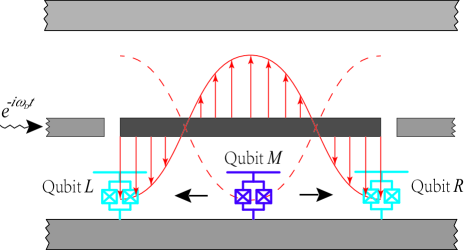
Illustrated in Fig. 1, the system comprises a cavity resonator made of a waveguide stripline and three superconducting qubits, where we use the indicators (left), (middle), and (right) to distinguish them. Then, using Pauli matrices for the two-level qubits of transition frequencies and a pair of creation and annihilation operators for the cavity field of frequency , the free energy part of the Hamiltonian () reads . The index ranges over . The interaction part corresponds to the qubit-resonator coupling, in the rotating-wave approximation, with individual (unequal) coupling strengths , and , letting the interaction Hamiltonian be . In such superconducting circuits, the physical dimension of qubits (on the scale of m) is much less than the inter-qubit spacings (commensurate with cavity wavelength, on the scale of cm) [24]. Hence, the direct inter-qubit coupling is neglected.
We consider qubit and qubit placed at the edges of the stripline resonator, i.e. located at antinodes of the cavity field, and thus always maximally coupled to the cavity field. Qubit is placed between the qubits and and we allow its location to be variable such that be tunable between the maximal coupling attained by (and ) and the minimal (vanishing) coupling if it is located at a field node. The cavity field is driven by an external microwave field with frequency and a weak driving amplitude [32], making the external part of the Hamiltonian be .
To derive the evolution dynamics of the quadripartite system, we first diagonalize the closed subsystem consisting of and . Under weak driving, only the low-excitation number states and of the cavity mode are considered, giving rise to 16 dressed states, transformable from the tensor product states contributed by the cavity mode and the qubit eigenstates. Hence, writing the dressed states as with associated eigen-energies , we have , where the index ranges over . The transformation between the dressed state and the bare states reads
| (1) |
where gives a decimal index converted from the binary combinations of the qubit states, where the ground state is designated by 0 and the excited state by 1. The state of the qubit (qubit ) indicates the most (least) significant bit, making range over the integers between 0 and 7. For example, . Also, indicates the transformation coefficients for the -th dressed state.
In the space spanned by the basis states of Eq. (1), the effect of the photonic creation and annihilation are distributed across all dressed states. Therefore, before we can derive the equation of motion of the system, we transform the operator that appears in into the dressed basis, i.e.
| (2) | |||||
where . Consequently, the total Hamiltonian is written as
| (3) |
Writing the time-dependent state vector as , we arrive at the Schrödinger equation of the coefficients :
| (4) |
In the following, the determination of entanglement will be carried out from the state coefficients under the bare-state basis, i.e. transforming back the dressed states, we have
| (5) |
for the vector .
III Evolution and four-tangle
The partitioning of the bipartite and the quadripartite entanglements that evolve with time is reflected in the coefficients . To be exact, we follow the definition of polynomial invariant [9] that generalizes 3-tangle [4] to measure distirbuted entanglement in arbitrary -partite systems. Here we customize this polynomial invariant to degree 4 to have
| (6) |
to reflect the entanglement distribution, thus the degree of monogamy, in the quadripartite system under study. In this customization,
| (7) |
indicates the concurrence between a -component subsystem and the rest parts [4, 9], where denotes the reduced density matrix for the components with the rest components traced out. The sum over in Eq. (6) is taken over all combinations of components out of the four (e.g. when , the index {2} includes the combination of qubit and qubit ). To simplify the terminology, we shall call Eq. (6) 4-tangle in the discussion below.
In the quadripartite system, the cavity field in the stripline resonator acts as a quantum bus that simultaneously couples to all three qubits. It serves, therefore, as a mediator that distributes entanglement among all components it couples to, similar to the role played by the mechanical resonator in a double-optical-cavity system [19]. Here, being driven by an external microwave field from the waveguide, the cavity field has its state vary over time and hence redistributes the entanglement among the qubits over time.
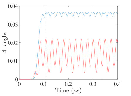
To observe the process of the redistribution and to decide whether the monogamous relation is obeyed, we consider an initial state which has the cavity mostly populated to initiate the entanglement. With full population at the one-photon state, i.e. , the distributed entanglement measured by the 4-tangle, as shown in Fig. 2, reaches a saturated value after the cavity field synchronizes the evolution of the qubits [20]. The saturated value is defined as the periodic peak obtainable by the 4-tangle and the synchronization duration is then the time between the start of the entanglement and the moment at which the first one of such peaks appears. Besides the rising time and the saturated value, the synchronization pattern is typical whether the couplings among the qubits are homogeneous or inhomogeneous. In the plot, we used experimentally accessible transition frequencies of transmon qubits at GHz and, to account for the discrepancies at fabrication [24], have let GHz. The cavity is slightly detuned from the qubits at GHz. The microwave field in the waveguide drives the cavity at kHz and propagates at GHz. For the homogeneous case, the coupling strength is set to MHz for all among ; for the inhomogeneous case, MHz and MHz. The differing aspects in the two scenarios is that homogeneous coupling permits a greater saturated 4-tangle at the expense of a slower rising time.
IV Periodicity in monogamy
From Fig. 2, we also observe periodicity in the variation, akin to the vanishing and revival effects observed in other entanglement studies, albeit neither case has the entanglement measure completely vanish where the monogamy relation would reduce to its equality limit. We find that the evolution of the 4-tangle in the quadripartite system is highly dependent on the initial state. With a slight alteration to the cavity photon, by letting while having qubit slightly inverted with at initial time, the monogamy equality can be asymptotically achieved, where the periodicity depends on all three coupling strengths , , and .
To obtain an appropriate coupling combination for a desired pair of revival period and 4-tangle magnitude, one should scan over the triple parameter space (). Nevertheless, since our goal is to seek the effect of asynchronous excitation on entanglement generation, the parameter space is compressed to 2-dimensional to simplify our study. We let qubits and be fixated at antinodes to receive the same maximal coupling () while allowing qubit to be removed from antinode to receive sub-maximal coupling characterized by the dimensionless parameter . In other words, the excitation rate of qubit is asynchronous with qubits and where the pair signifies the absolute coupling strength and the inhomogeneity of the couplings.
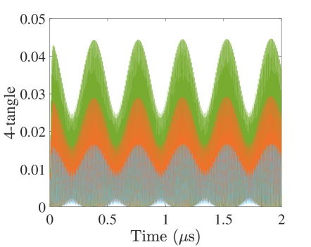
We first consider the homogeneous coupling scenario, i.e. . As shown in Fig. 3, the time evolution of the 4-tangle follows the pattern of Fig. 2 for all , which demonstrate periodic vanishing and revival patterns after a short duration of rising from initial zero value. Throughout, the alternating-sign sum of concurrences is found to be always non-negative, preserving the monogamy inequality in Eq. (6). Furthermore, irrespective of the coupling strength, the monogamy equality limit is reached at the same time instants. With the same system parameters as in Fig. 2, the period is measured at s. The amplitude of 4-tangle monotonically follows the coupling strength .
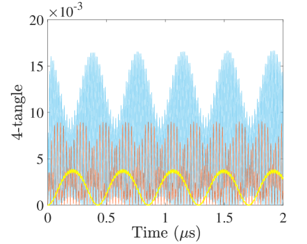
For the inhomogeneous scenario, which can be implemented by removing the qubit from the antinode of the cavity field as indicated in Fig. 1, the periodic patterns of the 4-tangle evolution are reflected in Fig. 4. In the plot, the coupling strengths and are let fixed at MHz, while the relative coupling parameter takes the values , , and . The unity case (given by the blue curve) indicates the homogeneous coupling and is the same of the one shown in Fig. 3. Using it as a reference, we observe that lowering and thereby permitting inhomogeneous excitation to the middle qubit leads to a monotonic decrease in the oscillating amplitude of the entanglement, but the period of oscillation is affected in a non-monotonic way.
During the evolution, the amplitude of oscillation in the 4-tangle varies over time while the period between one asymptotic vanishing and the next remains fixed. When is reduced from 1 to 0.5, the maximum amplitude decreases to about half the original amplitude while the period is reduced from s to s. When is further reduced from 0.5 to 0.05, the maximum amplitude is reduced by about 95%, whereas the period , on the contrary, increases from s to s.
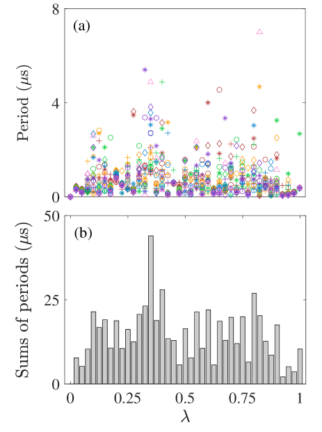
Overall, the dependence of the period on the is highly nonlinear and not extractable analytically from the expression of Eq. (6). We resort to a statistical method to characterize this dependence. We have computed the evolutions of the 4-tangle when varies between zero and one over a range of values of coupling strength and extracted the periods from the plots for different combinations of and . Using a scatter plot of Fig. 5, we mark each extracted period as a data point, which is color- and symbol-coded as in Fig. 5(a), and binned the data points into slots each differing from the neighboring slot by , within which the values of the data points are summed as in Fig. 5(b). For each slot of , varies between MHz and MHz at MHz intervals and the other system parameters remain identical to those used in the figures above.
Therefore, Fig. 5 shows on average how likely a combination of would generate a longer period in 4-tangle. We observe that, statistically speaking, this period maximizes at , where the scatter datapoints have the greatest accumulated value and thus one is most likely to obtain a long revival period at this regardless the absolute coupling strength . In constrast, it is less likely at and least likely at . In particular, though one datapoint at corresponds to a long period in (a), its binned sum is less than that of , showing it is less likely on average to obtain a long period at when all values are considered.
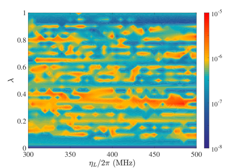
To obtain a better resolution of the variation of period against , we have further conducted simulations running at MHz intervals for , while retaining an interval of along the -axis, and summarize the results in the contour plot in Fig. 6. The period is log-scaled and plotted in color against and . First, verifying the findings from Fig. 5, maximizes at the inhomogeneous couplings of while minimizes at the two ends and the middleway of . Secondly, at the maximizing values of , the dependence of on the absolute coupling is not uniform, showing also a nonlinear relationship. Therefore, if one considers prolonging the duration of entanglement for the purpose of processing quantum information in a multi-qubit system, uniform couplings among the qubits are not necessarily beneficial. Rather, inhomogeneous coupling peculiar to the system setting can provide a means of assistance. For example, for the quadripartite qubit-cavity system under study, given the same transmon qubit transition frequencies as in Sec. IIIA, the longest period appears at MHz. For a stripline cavity of length mm [23], this signifies a setup that prolongs the duration of entanglement by moving the middle qubit as shown in Fig. 1 to the position mm from the center antinode.
V Conclusions
We have studied the dynamic evolution of the entanglement measure 4-tangle, which is a polynomial invariant that quantifies the degree of separation of the monogamous entanglements from the group entanglements, for a quadripartite system consisting of three qubits and one cavity mode. We find that the 4-tangle throughout the interactive evolution of the qubits is guaranteed non-negative and exhibits periodic revival. Under the framework of circuit QED with three qubits, it is shown that it inhomogeneity of couplings that induces asynchronous excitations to the qubits facilitate the choice of entanglement generation. By selecting a combination of absolute relative coupling strengths among the qubits, one can not only obtain the desired distributed entanglement for generating GHZ states, but also determine how soon the entanglement is realized.
For instance, in some cases when fast generation of entanglement is desired, one can place all three qubits on the antinodes for homogeneous maximal couplings or allow the middle qubit to be placed midway towards a neighboring node where the effective coupling is half of the possible maximum. In some other cases, slow generation might be wanted, such as when longer rise and fall times in entanglement are desired to tolerate the timing inaccuracies of the experimental apparatus, so that the fidelity of actual target state would be improved. In such cases, one can move the middle qubit to the place where the coupling is about one-third of the maximum while retaining the other two qubits at the antinodes.
We note that the study here is limited to three cavity-coupled qubits. Generalization to larger number of qubits with a parameter space of higher dimensions require future works in this direction. Also, the methodology we use here is based on statistical and numerical analysis. Alternative approaches are needed to seek an analytical optimization method for finding entanglement characteristics such as the extremal periods.
Acknowledgements.
H. I. thanks the support by the Science and Technology Development Fund, Macau SAR (File no. 0130/2019/A3) and by University of Macau (MYRG2018-00088-IAPME).References
- [1] K. Chen and H.-K. Lo, Quan. Inf. Comput. 7, 689 (2007).
- [2] T. Gao, F. L. Yan, and Z. X. Wang, J. Phys. A: Math. Gen. 38, 5761 (2005).
- [3] A. W. Chin, S. F. Huelga, and M. B. Plenio, Phys. Rev. Lett. 109, 233601 (2012).
- [4] V. Coffman, J. Kundu, and W. K. Wootters, Phys. Rev. A 61, 052306 (2000).
- [5] W. K. Wootters, Phys. Rev. Lett. 80, 2245 (1998).
- [6] R. Horodecki, P. Horodecki, M. Horodecki, and K. Horodecki, Rev. Mod. Phys. 81, 865 (2009).
- [7] T. J. Osborne and F. Verstraete, Phys. Rev. Lett. 96, 220503 (2006).
- [8] M. F. Cornelio, Phys. Rev. A 87,032330 (2013).
- [9] C. Eltschka, T. Bastin, A. Osterloh, and J. Siewert, Phys. Rev. A 85, 022301 (2012).
- [10] A. Wong and N. Christensen, Phys. Rev. A 63, 044301 (2001).
- [11] F. Mintert, M. Kuś, and A. Buchleitner, Phys. Rev. Lett. 95, 260502 (2005).
- [12] F. Mintert, A. R. R. Carvalho, M. Kuś, and A. Buchleitner, Phys. Rep. 415, 207 (2005).
- [13] W. Dür, G. Vidal, and J. I. Cirac, Phys. Rev. A 62, 062314 (2000).
- [14] B. Regula, A. Osterloh, and G. Adesso, Phys. Rev. A 93, 052338 (2016).
- [15] S. Gartzke and A. Osterloh, Phys. Rev. A 98, 052307 (2018).
- [16] T. R. de Oliveira, M. F. Cornelio, and F. F. Fanchini, Phys. Rev. A 89, 034303 (2014).
- [17] Y.-K. Bai, Y.-F. Xu, and Z. D. Wang, Phys. Rev. Lett. 113, 100503 (2014).
- [18] Y. Liu, S. Kuang, and S. Cong, IEEE Trans. Cyber. 47, 3827 (2017).
- [19] T. Huan, R. Zhou, and H. Ian, Phys. Rev. A 92, 022301 (2015).
- [20] T. Huan, R. Zhou, and H. Ian, Sci. Rep. 10, 12975 (2020).
- [21] A. Nourmandipour, M. K. Tavassoly, and M. Rafiee, Phys. Rev. A 93, 022327 (2016).
- [22] Y.-J. Zhang, Z.-X. Man, X.-B. Zou, Y.-J. Xia, and G.-C. Guo, J. Phys. B: At. Mol. Opt. Phys. 43, 045502 (2010).
- [23] A. Wallraff, D. I. Schuster, A. Blais, L. Frunzio, R.-S. Huang, J. Majer, S. Kumar, S. M. Girvin, and R. J. Schoelkopf, Nature 431, 162 (2004).
- [24] J. M. Fink, R. Bianchetti, M. Baur, M. Göppl, L. Steffen, S. Filipp, P. J. Leek, A. Blais, and A. Wallraff, Phys. Rev. Lett. 103, 083601 (2009).
- [25] H. Ian, Y. Liu, and F. Nori, Phys. Rev. A 85, 053833 (2012).
- [26] H. Ian and Y. Liu, Phys. Rev. A 89, 043804 (2014).
- [27] H. Ian, EPL 114, 50005 (2016).
- [28] Z. Ficek and R. Tanaś, Phys. Rev. A 74, 024304 (2006).
- [29] M. Dukalski and Ya. M. Blanter, Phys. Rev. A 82, 052330 (2010).
- [30] G. Wang, L. Huang, Y.-C. Lai, and C. Grebogi, Phys. Rev. Lett. 112, 110406 (2014).
- [31] M. Kjaergaard, M. E. Schwartz, J. Braumüller, P. Krantz, J. I.-J. Wang, S. Gustavsson, and W. D. Oliver, Superconducting Qubits: Current State of Play, Annu. Rev. Condens. Matter Phys. 11, 369 (2020).
- [32] K. Børkje, A. Nunnenkamp, J. D. Teufel, and S. M. Girvin, Phys. Rev. Lett. 111, 053603 (2013).