This paper was converted on www.awesomepapers.org from LaTeX by an anonymous user.
Want to know more? Visit the Converter page.

Distributed Mirror Descent Algorithm with Bregman Damping for Nonsmooth Constrained Optimization

Guanpu Chen, Weijian Li, Gehui Xu, and Yiguang Hong This work was supported in part by Shanghai Municipal Science and Technology Major Project under Grant 2021SHZDZX0100, and in part by the National Natural Science Foundation of China under Grant 61733018. (Corresponding author: Yiguang Hong)G. Chen and G. Xu is with Key Laboratory of Systems and Control, Academy of Mathematics and Systems Science, Beijing, China, and is also with School of Mathematical Sciences, University of Chinese Academy of Sciences, Beijing, China. chengp@amss.ac.cn, xghapple@amss.ac.cnW. Li is with Department of Automation, University of Science and Technology of China, Hefei, Anhui, China. ustcwjli@mail.ustc.edu.cnY. Hong is with Department of Control Science and Engineering & Shanghai Research Institute for Intelligent Autonomous Systems, Tongji University, Shanghai, China, and is also with the Key Laboratory of Systems and Control, Academy of Mathematics and Systems Science, Beijing, China. yghong@iss.ac.cn
Abstract

To solve distributed optimization efficiently with various constraints and nonsmooth functions, we propose a distributed mirror descent algorithm with embedded Bregman damping, as a generalization of conventional distributed projection-based algorithms. In fact, our continuous-time algorithm well inherits good capabilities of mirror descent approaches to rapidly compute explicit solutions to the problems with some specific constraint structures. Moreover, we rigorously prove the convergence of our algorithm, along with the boundedness of the trajectory and the accuracy of the solution.

I INTRODUCTION

Distributed optimization has served as a hot topic in recent years for its broad applications in various fields such as sensor networks and smart grids [1, 2, 3, 4, 5, 6, 7]. Under multi-agent frameworks, the global cost function consists of agents’ local ones, and each agent shares limited information with its neighbors through a network to achieve an optimal solution. Meanwhile, distributed continuous-time algorithms have been well developed thanks to system dynamics and control theory [8, 9, 10, 11, 12].

Up to now, various approaches have been employed for distributed design of constrained optimization. Intuitively, implementing projection operations on local constraints is a most popular method, such as projected proportional-integral protocol [8] and projected dynamics with constraints based on KKT conditions [9]. In addition, other approaches such as distributed primal-dual dynamics and penalty-based algorithms [10, 11, 12] also perform well provided that constraints are endowed with specific expressions. However, time complexity in finding optimal solutions with complex or high-dimensional constraints forces researchers to exploit efficient approaches for special constraint structures, such as the unit simplex and the Euclidean sphere.

In fact, the mirror descent (MD) method serves as a powerful tool for solving constrained optimization. As we know, first introduced in [13], MD is regarded as a generalization of (sub)gradient methods. With mapping the variables into a conjugate space, MD employs the Bregman divergence and performs well in handling local constraints with specific structures [14, 15, 16]. This process results in a faster convergence rate than that of projected (sub)gradient descent algorithms, especially for large-scale optimization problems. Undoubtedly, as such an important tool, MD has played a crucial role in various distributed algorithm designs, as given in [17, 18, 19, 20].

In recent years, continuous-time MD-based algorithms have also attracted much attention. For example, [14] proposed the acceleration of a continuous-time MD algorithm, and afterward, [21] showed continuous-time stochastic MD for strongly convex functions, while [22] proposed a discounted continuous-time MD dynamics to approximate the exact solution. In the distributed design, although [19] presented a distributed MD dynamics with integral feedback, the result merely achieved optimal consensus and part variables turn to be unbounded. Due to the booming development and extensive demand of distributed design, distributed continuous-time MD-based methods need more exploration and development actually.

Therefore, we study continuous-time MD-based algorithms to solve distributed nonsmooth optimization with local and coupled constraints. The main contributions of this note can be summarized as follows. We propose a distributed continuous-time mirror descent algorithm by introducing the Bregman damping, which can be regarded as a generalization of classic distributed projection-based dynamics [8, 23] by taking the Bregman damping in a quadratic form. Moreover, our algorithm well inherits the good capabilities of MD-based approaches to rapidly compute explicit solutions to the problems with some concrete constraint structures like the unit simplex or the Euclidean sphere. With the designed Bregman damping, our MD-based algorithm makes all the variables’ trajectories bounded, which could not be ensured in [14, 19], and avoids the inaccuracy of the convergent point occurred in [22].

The remaining part is organized as follows. Section II gives related preliminary knowledge. Next, Section III formulates the distributed optimization and provides our algorithm, while Section IV presents the main results. Then, Section V provides illustrative numerical examples. Finally, Section VI gives the conclusion.

II Preliminaries

In this section, we give necessary notations and related preliminary knowledge.

II-A Notations

Denote n\mathbb{R}^{n} (or m×n\mathbb{R}^{m\times n}) as the set of nn-dimensional (or mm-by-nn) real column vectors (or real matrices), and InI_{n} as the n×nn\times n identity matrix. Let 1n{1}_{n} (or 0n{0}_{n}) be the nn-dimensional column vector with all entries of 11 (or 0). Denote ABA\otimes B as the Kronecker product of matrices AA and BB. Take col{x1,,xn}=col{xi}i=1n=(x1T,,xnT)Tcol\{x_{1},\dots,x_{n}\}=col\{x_{i}\}_{i=1}^{n}=(x_{1}^{\rm T},\dots,x_{n}^{\rm T})^{\rm T}, \|\cdot\| as the Euclidean norm, and rint(C)\text{rint}(C) as the relative interior of the set CC [24].

An undirected graph can be defined by 𝒢(𝒱,)\mathcal{G}(\mathcal{V},\mathcal{E}), where 𝒱={1,,n}\mathcal{V}=\{1,\ldots,n\} is the set of nodes and 𝒱×𝒱\mathcal{E}\subset\mathcal{V}\times\mathcal{V} is the set of edges. Let 𝒜=[aij]n×n\mathcal{A}=[a_{ij}]\in\mathbb{R}^{n\times n} be the adjacency matrix of 𝒢\mathcal{G} such that aij=aji>0a_{ij}=a_{ji}>0 if {j,i}\{j,i\}\in\mathcal{E}, and aij=0a_{ij}=0, otherwise. The Laplacian matrix is Ln=𝒟𝒜L_{n}=\mathcal{D}-\mathcal{A}, where 𝒟=diag{Dii}n×n\mathcal{D}=\text{diag}\{D_{ii}\}\in\mathbb{R}^{n\times n} with 𝒟ii=j=1naij\mathcal{D}_{ii}=\sum_{j=1}^{n}a_{ij}. If the graph 𝒢\mathcal{G} is connected, then ker(Ln)={k1n:k}\text{ker}(L_{n})=\{k{1}_{n}:k\in\mathbb{R}\}.

II-B Convex analysis

For a closed convex set Ωn\Omega\subseteq\mathbb{R}^{n}, the projection map PΩ:nΩP_{\Omega}:\mathbb{R}^{n}\rightarrow\Omega is defined as PΩ(x)=argminyΩxyP_{\Omega}(x)=\text{argmin}_{y\in\Omega}\|x-y\|. Especially, denote [x]+P+n(x)[x]^{+}\triangleq P_{\mathbb{R}^{n}_{+}}(x) for convenience. For xΩx\in\Omega, denote the normal cone to Ω\Omega at xx by

𝒩Ω(x)={vn:vT(yx)0,yΩ}.\mathcal{N}_{\Omega}(x)=\big{\{}v\in\mathbb{R}^{n}:v^{\rm T}(y-x)\leq 0,\quad\forall y\in\Omega\big{\}}.

A continuous function f:nf:\mathbb{R}^{n}\rightarrow\mathbb{R} is ω\omega-strongly convex on Ω\Omega if

(xy)T(gxgy)ωxy2,x,yC,(x-y)^{\rm T}(g_{x}-g_{y})\geq\omega\|x-y\|^{2},\,\forall x,y\in C,

where ω>0\omega>0, gxf(x)g_{x}\in\partial f(x), and gyf(y)g_{y}\in\partial f(y).

The Bregman divergence based on the differentiable generating function f:Ωf:\Omega\rightarrow\mathbb{R} is defined as

Df(x,y)=f(x)f(y)f(y)T(xy),x,yΩ.\displaystyle D_{f}(x,y)=f(x)-f(y)-\nabla f(y)^{T}(x-y),\,\forall x,y\in\Omega.

The convex conjugate function of ff is defined as

f(z)=supxΩ{xTzf(x)}.\displaystyle f^{*}(z)=\sup_{x\in\Omega}\big{\{}x^{T}z-f(x)\big{\}}.

The following lemma reveals a classical conclusion about convex conjugate functions, of which readers can find more details in [13, 15].

Lemma 1

Suppose that a function ff is differentiable and strongly convex on a closed convex set Ω\Omega. Then f(z)f^{*}(z) is convex and differentiable, and f(z)=minxΩ{xTz+f(x)}f^{*}(z)=\min_{x\in\Omega}\big{\{}-x^{T}z+f(x)\big{\}}. Moreover, f(z)=ΠΩf(z)\nabla f^{*}(z)=\Pi_{\Omega}^{f}(z), where

ΠΩf(z)argminxΩ{xTz+f(x)}.\displaystyle\Pi_{\Omega}^{f}(z)\triangleq\mathop{\text{argmin}}_{x\in\Omega}\big{\{}-x^{T}z+f(x)\big{\}}. (1)

II-C Differential inclusion

A differential inclusion is given by

x˙(t)=(x(t)),x(0)=x0,t0,\dot{x}(t)=\mathcal{F}(x(t)),~{}x(0)=x_{0},~{}t\geq 0, (2)

where :nn\mathcal{F}:\mathbb{R}^{n}\rightrightarrows\mathbb{R}^{n} is a set-valued map. \mathcal{F} is upper semi-continuous at xx if there exists δ>0\delta>0 for all ϵ>0\epsilon>0 such that

(y)(x)+B(0;ϵ),yB(x;δ)\mathcal{F}(y)\subset\mathcal{F}(x)+B(0;\epsilon),~{}\forall y\in B(x;\delta)

and it is upper semi-continuous if it is so for all xnx\in\mathbb{R}^{n}. A Caratheodory solution to (2) defined on [0,τ)[0,+)[0,\tau)\subset[0,+\infty) is an absolutely continuous function x:[0,τ)nx:[0,\tau)\rightarrow\mathbb{R}^{n} satisfying (2) for almost all t[0,τ)t\in[0,\tau) in Lebesgue measure [25]. The solution x(t)x(t) is right maximal if it has no extension in time. A set \mathcal{M} is said to be weakly (strongly) invariant with respect to (2) if \mathcal{M} contains a (all) maximal solution to (2) for any x0x_{0}\in\mathcal{M}. If 0n(xe)0_{n}\in\mathcal{F}(x_{e}), then xex_{e} is an equilibrium point of (2). The existence of a solution to (2) is guaranteed by the following lemma [25].

Lemma 2

If \mathcal{F} is locally bounded, upper semicontinuous, and takes nonempty, compact and convex values, then there exists a Caratheodory solution to (2) for any initial value.

Let V:nV:\mathbb{R}^{n}\rightarrow\mathbb{R} be a locally Lipschitz continuous function, and V(x)\partial V(x) be the Clarke generalized gradient of VV at xx. The set-valued Lie derivative for VV is defined by V(x){a:a=pTv,pV(x),v(x)}\mathcal{L}_{\mathcal{F}}V(x)\triangleq\{a\in\mathbb{R}:a=p^{T}v,p\in\partial V(x),v\in\mathcal{F}(x)\}. Let maxV(x)\max\mathcal{L}_{\mathcal{F}}V(x) be the largest element of V(x)\mathcal{L}_{\mathcal{F}}V(x). Referring to [25], we have the following invariance principle for (2).

Lemma 3

Suppose that \mathcal{F} is upper semi-continuous and locally bounded, and (x)\mathcal{F}(x) takes nonempty, compact, and convex values. Let V:nV:\mathbb{R}^{n}\rightarrow\mathbb{R} be a locally Lipschitz and regular function, 𝒮n\mathcal{S}\subset\mathbb{R}^{n} be compact and strongly invariant for (2), and ψ(t)\psi(t) be a solution to (2). Take

={xn:0V(x)},\mathcal{R}=\{x\in\mathbb{R}^{n}:0\in\mathcal{L}_{\mathcal{F}}V(x)\},

and \mathcal{M} as the largest weakly invariant subset of ¯𝒮\bar{\mathcal{R}}\cap\mathcal{S}, where ¯\bar{\mathcal{R}} is the closure of \mathcal{R}. If maxV(x)0\max\mathcal{L}_{\mathcal{F}}V(x)\leq 0 for all x𝒮x\in\mathcal{S}, then limtdist(ψ(t),)=0\lim_{t\to\infty}{\rm dist}(\psi(t),\mathcal{M})=0.

III Formulation and algorithm

In this paper, we consider a nonsmooth optimization problem with both local and coupled constraints. There are NN agents indexed by 𝒱={1,,N}\mathcal{V}=\{1,\dots,N\} in a network 𝒢(𝒱,)\mathcal{G}(\mathcal{V},\mathcal{E}). For agent ii, the decision variable is xix_{i}, the local feasible set is Ωin\Omega_{i}\subseteq\mathbb{R}^{n}, and the local cost function is fi:nf_{i}:\mathbb{R}^{n}\rightarrow\mathbb{R}. Define 𝛀=i=1NΩi\bm{\Omega}=\prod_{i=1}^{N}\Omega_{i} and 𝒙=col{xi}i=1N\bm{x}=\text{col}\{x_{i}\}_{i=1}^{N}. All agents cooperate to solve the following distributed optimization:

min𝒙𝛀\displaystyle\min_{\bm{x}\in\bm{\Omega}} i=1Nfi(xi)\displaystyle\;\sum_{i=1}^{N}f_{i}(x_{i})
s.t. i=1Ngi(xi)0p,i=1NAixibi=0q,\displaystyle\;\sum_{i=1}^{N}g_{i}(x_{i})\leq 0_{p},\quad\sum_{i=1}^{N}A_{i}x_{i}-b_{i}=0_{q}, (3)

where gi:npg_{i}:\mathbb{R}^{n}\rightarrow\mathbb{R}^{p}, Aiq×nA_{i}\in\mathbb{R}^{q\times n} and biqb_{i}\in\mathbb{R}^{q}, for i𝒱i\in\mathcal{V}. Except for the local constraint 𝛀\bm{\Omega}, other constraints in (III) are said to be coupled ones since the solutions rely on global information. In the multi-agent network, agent ii only has the local decision variable xiΩix_{i}\in\Omega_{i}, and moreover, the local information fif_{i}, gig_{i}, AiA_{i} and bib_{i}. Thus, agents need communication with neighbors through the network 𝒢\mathcal{G}.

Actually, MD replaces the Euclidean regularization in (sub)gradient descent algorithms with Bregman divergence. In return, different generating functions of Bregman divergence may efficiently bring explicit solutions on different special feasible sets. For example, if ϕ(x)=12x2\phi(x)=\frac{1}{2}\|x\|^{2} and Ω\Omega is convex and closed, then

ΠΩϕ(z)=argminxΩ12xz2=PΩ(z),\displaystyle\Pi_{\Omega}^{\phi}(z)=\mathop{\text{argmin}}_{x\in\Omega}\frac{1}{2}\|x-z\|^{2}=P_{\Omega}(z), (4)

which actually turns into the classical Euclidean regularization with projection operations. Furthermore, if Ω={x+n:k=1nxk=1}\Omega=\{x\in\mathbb{R}^{n}_{+}:\sum_{k=1}^{n}x^{k}=1\} and ϕ(x)=k=1nxklog(xk)\phi(x)=\sum_{k=1}^{n}x^{k}\log(x^{k}) with the convention 0log0=00\log 0=0, then

ΠΩϕ(z)=col{exp(zk)j=1nexp(zj)}k=1n,\displaystyle\Pi_{\Omega}^{\phi}(z)=\text{col}\Big{\{}\frac{\exp(z^{k})}{\sum_{j=1}^{n}\exp(z^{j})}\Big{\}}_{k=1}^{n}, (5)

which is the well-known KL-divergence on the unit simplex.

Assign a generating function ϕi:n\phi_{i}:\mathbb{R}^{n}\rightarrow\mathbb{R} of the Bregman divergence to each agent i𝒱i\in\mathcal{V}. Then we consider the following assumptions for (III).

Assumption 1
  1. (i)

    For i𝒱i\in\mathcal{V}, Ωi\Omega_{i} is closed and convex, fif_{i} and gig_{i} are convex on Ωi\Omega_{i}, and moreover, ϕi\phi_{i} is differentiable and strongly convex on Ωi\Omega_{i}.

  2. (ii)

    There exists at least one 𝒙rint(𝛀)\bm{x}\in\text{rint}(\bm{\Omega}) such that i=1Ngi(xi)<0p\sum_{i=1}^{N}g_{i}(x_{i})<0_{p} and i=1NAixibi=0q\sum_{i=1}^{N}A_{i}x_{i}-b_{i}=0_{q}.

  3. (iii)

    The undirected graph 𝒢\mathcal{G} is connected.

Remark 1

Clearly, (III) can be regarded as a generalization for both distributed optimal consensus problems [26, 12, 19] and distributed resource allocation problems [27, 23]. Moreover, gig_{i} in the coupled constraints may not required to be affine, which is more general than the constraints in previous works [10, 28]. Also, the problem setting does not require strongly or strictly convexity for either cost functions fif_{i} or constraint functions gig_{i} [27, 10], and the selection qualification for generating function ϕi\phi_{i} has also been widely used [19, 14, 22].

For designing a distributed algorithm, we introduce auxiliary variables ωip\omega_{i}\in\mathbb{R}^{p}, νiq\nu_{i}\in\mathbb{R}^{q}, λip\lambda_{i}\in\mathbb{R}^{p}, μiq\mu_{i}\in\mathbb{R}^{q}, yiny_{i}\in\mathbb{R}^{n} and γip\gamma_{i}\in\mathbb{R}^{p} for each agent i𝒱i\in\mathcal{V}. Moreover, we employ the gradient ϕi\nabla\phi_{i} of generating functions as the Bregman damping in the algorithm, which ensures the trajectories’ boundedness [14, 19] and avoids the convergence inaccuracy [22]. Recall that aija_{ij} is the (i,j)(i,j)-th entry of the adjacency matrix 𝒜\mathcal{A} and ΠΩiϕi()\Pi_{\Omega_{i}}^{\phi_{i}}(\cdot) is defined in (1). Then we propose a distributed mirror descent algorithm with Bregman damping (MDBD) for (III).

Algorithm 1 MDBD for i𝒱i\in\mathcal{V}

Initialization:
xi(0)Ωix_{i}(0)\in\Omega_{i}, yi(0)=0ny_{i}(0)=0_{n}, λi(0)=0p\lambda_{i}(0)=0_{p}, γi(0)=0p\gamma_{i}(0)=0_{p},
ωi(0)=0p\omega_{i}(0)=0_{p}, μi(0)=0q\mu_{i}(0)=0_{q}, νi(0)=0q\nu_{i}(0)=0_{q};
take a proper generating function ϕi()\phi_{i}(\cdot) according to Ωi\Omega_{i}.
Flows renewal:

y˙i\displaystyle\dot{y}_{i}\, fi(xi)gi(xi)TλiAiTμi+ϕi(xi)yi,\displaystyle{\in}-{\partial}f_{i}(x_{i})-{\partial}g_{i}(x_{i})^{\rm T}\lambda_{i}-A_{i}^{\rm T}\mu_{i}+\nabla\phi_{i}(x_{i})-y_{i},
γ˙i\displaystyle\dot{\gamma}_{i} =gi(xi)j=1Naij(ωiωj)+λiγi,\displaystyle=g_{i}(x_{i})-\sum_{j=1}^{N}a_{ij}(\omega_{i}-\omega_{j})+\lambda_{i}-\gamma_{i},
μ˙i\displaystyle\dot{\mu}_{i} =Aixibij=1Naij(νiνj),\displaystyle=A_{i}x_{i}-b_{i}-\sum_{j=1}^{N}a_{ij}(\nu_{i}-\nu_{j}),
ω˙i\displaystyle\dot{\omega}_{i} =j=1Naij(λiλj),\displaystyle=\sum_{j=1}^{N}a_{ij}(\lambda_{i}-\lambda_{j}),
ν˙i\displaystyle\dot{\nu}_{i} =j=1Naij(μiμj),\displaystyle=\sum_{j=1}^{N}a_{ij}(\mu_{i}-\mu_{j}),
xi\displaystyle x_{i} =ΠΩiϕi(yi),\displaystyle=\Pi_{\Omega_{i}}^{\phi_{i}}(y_{i}),
λi\displaystyle\lambda_{i} =[γi]+.\displaystyle=[\gamma_{i}]^{+}.

In Algorithm 1, for each agent i𝒱i\in\mathcal{V}, information like fi{\partial}f_{i}, gi{\partial}g_{i}, AiA_{i} and bib_{i} serves as private knowledge, and values like ωi\omega_{i}, νi\nu_{i}, λi\lambda_{i} and μi\mu_{i} should be exchanged with neighbors through the network 𝒢\mathcal{G}. Moreover, generating function ϕi\phi_{i} and Bregman damping ϕi\nabla\phi_{i} can be determined privately and individually, not necessarily identical. It follows from Lemma 2 that the existence of a Caratheodory solution to Algorithm 1 can be guaranteed.

For simplicity, define

𝝀=col{λi}i=1NNp,𝝁=col{μi}i=1NNq,\bm{\lambda}=\text{col}\big{\{}\lambda_{i}\big{\}}_{i=1}^{N}\in\mathbb{R}^{Np},~{}~{}\bm{\mu}=\text{col}\big{\{}\mu_{i}\big{\}}_{i=1}^{N}\in\mathbb{R}^{Nq},
𝝎=col{ωi}i=1NNp,𝝂=col{νi}i=1NNq,\bm{\omega}=\text{col}\big{\{}\omega_{i}\big{\}}_{i=1}^{N}\in\mathbb{R}^{Np},~{}~{}\bm{\nu}=\text{col}\big{\{}\nu_{i}\big{\}}_{i=1}^{N}\in\mathbb{R}^{Nq},
𝒚=col{yi}i=1NNn,𝜸=col{γi}i=1NNp.\bm{y}=\text{col}\big{\{}y_{i}\big{\}}_{i=1}^{N}\in\mathbb{R}^{Nn},~{}~{}\bm{\gamma}=\text{col}\big{\{}\gamma_{i}\big{\}}_{i=1}^{N}\in\mathbb{R}^{Np}.

Let 𝚯=𝛀×+Np×N(p+2q)\bm{\Theta}=\bm{\Omega}\times\mathbb{R}^{Np}_{+}\times\mathbb{R}^{N(p+2q)}, and moreover,

𝒛=col{𝒙,𝝀,𝝁,𝝎,𝝂},𝒔=col{𝒚,𝜸,𝝁,𝝎,𝝂}.\bm{z}=\text{col}\{\bm{x},\bm{\lambda},\bm{\mu},\bm{\omega},\bm{\nu}\},\quad\bm{s}=\text{col}\{\bm{y},\bm{\gamma},\bm{\mu},\bm{\omega},\bm{\nu}\}.

Take the Lagrangian function :𝚯\mathcal{L}:\bm{\Theta}\rightarrow\mathbb{R} as

(𝒛)=\displaystyle\mathcal{L}(\bm{z})= i=1Nfi(xi)+i=1NλiT(gi(xi)j=1Naij(ωiωj))\displaystyle\sum_{i=1}^{N}f_{i}(x_{i})+\sum_{i=1}^{N}\lambda_{i}^{T}\big{(}g_{i}(x_{i})-\sum_{j=1}^{N}a_{ij}(\omega_{i}-\omega_{j})\big{)}
+i=1NμiT(Aixibij=1Naij(νiνj)).\displaystyle+\sum_{i=1}^{N}\mu_{i}^{T}\big{(}A_{i}x_{i}-b_{i}-\sum_{j=1}^{N}a_{ij}(\nu_{i}-\nu_{j})\big{)}. (6)

For such a distributed convex optimization (III) with a zero dual gap, 𝒙𝛀\bm{x}^{\star}\in\bm{\Omega} is an optimal solution to problem (III) if and only if there exist auxiliary variables (𝝀,𝝁,𝝎,𝝂)+Np×N(p+2q)(\bm{\lambda}^{\star},\bm{\mu}^{\star},\bm{\omega}^{\star},\bm{\nu}^{\star})\in\mathbb{R}^{Np}_{+}\times\mathbb{R}^{N(p+2q)}, such that 𝒛=col{𝒙,𝝀,𝝁,𝝎,𝝂}\bm{z}^{\star}=\text{col}\{\bm{x}^{\star},\bm{\lambda}^{\star},\bm{\mu}^{\star},\bm{\omega}^{\star},\bm{\nu}^{\star}\} is a saddle point of \mathcal{L} [23], that is, for arbitrary 𝒛𝚯\bm{z}\in\bm{\Theta},

(𝒙,𝝀,𝝁,𝝎,𝝂)(𝒙,𝝀,\displaystyle\mathcal{L}(\bm{x}^{\star},\bm{\lambda},\bm{\mu},\bm{\omega}^{\star},\bm{\nu}^{\star})\leq\mathcal{L}(\bm{x}^{\star},\bm{\lambda}^{\star}, 𝝁,𝝎,𝝂)\displaystyle\bm{\mu}^{\star},\bm{\omega}^{\star},\bm{\nu}^{\star})
\displaystyle\leq (𝒙,𝝀,𝝁,𝝎,𝝂).\displaystyle\mathcal{L}(\bm{x},\bm{\lambda}^{\star},\bm{\mu}^{\star},\bm{\omega},\bm{\nu}).

Define

F(𝒛)=[col{fi(xi)+gi(xi)Tλi+AiTμi}i=1Ncol{gi(xi)}i=1N+𝑳p𝒘col{Aixi+bi}i=1N+𝑳q𝝂𝑳p𝝀𝑳q𝝁],\displaystyle F(\bm{z})=\begin{bmatrix}\text{col}\big{\{}{\partial}f_{i}(x_{i})+{\partial}g_{i}(x_{i})^{\rm T}\lambda_{i}+A_{i}^{\rm T}\mu_{i}\big{\}}_{i=1}^{N}\\ \text{col}\big{\{}-g_{i}(x_{i})\big{\}}_{i=1}^{N}+\bm{L}_{p}\bm{w}\\ \text{col}\big{\{}-A_{i}x_{i}+b_{i}\big{\}}_{i=1}^{N}+\bm{L}_{q}\bm{\nu}\\ -\bm{L}_{p}\bm{\lambda}\\ -\bm{L}_{q}\bm{\mu}\end{bmatrix}, (7)

where 𝑳p=LNIp\bm{L}_{p}=L_{N}\otimes I_{p} and 𝑳q=LNIq\bm{L}_{q}=L_{N}\otimes I_{q}. In fact, 𝒛\bm{z}^{\star} is a saddle point of \mathcal{L} if and only if F(𝒛)𝒩𝚯(𝒛)-F(\bm{z}^{\star})\in\mathcal{N}_{\bm{\Theta}}({\bm{z}}^{\star}), which was obtained in [27, 23, 10].

Hence, Algorithm 1 can be presented in the following compact form:

{𝒔˙F(𝒛)+Φ(𝒛)𝒔,𝒛=Π𝚯Φ(𝒔),\left\{\begin{aligned} \dot{\bm{s}}\;{\in}&-F(\bm{z})+\nabla\Phi(\bm{z})-\bm{s},\\ \bm{z}=&\;\Pi_{\bm{\Theta}}^{\Phi}(\bm{s}),\end{aligned}\right. (8)

where

Φ(𝒛)\displaystyle\nabla\Phi(\bm{z})\triangleq col{col{ϕi(xi)}i=1N,col{λi}i=1N,\displaystyle\text{col}\Big{\{}\text{col}\{\nabla\phi_{i}(x_{i})\}_{i=1}^{N},\text{col}\{\lambda_{i}\}_{i=1}^{N},
col{μi}i=1N,col{ωi}i=1N,col{νi}i=1N},\displaystyle\quad\text{col}\{\mu_{i}\}_{i=1}^{N},\text{col}\{\omega_{i}\}_{i=1}^{N},\text{col}\{\nu_{i}\}_{i=1}^{N}\Big{\}}, (9a)
Π𝚯Φ(𝒔)\displaystyle\Pi_{\bm{\Theta}}^{\Phi}(\bm{s})\triangleq col{col{ΠΩiϕi(yi)}i=1N,col{[γi]+}i=1N,\displaystyle\text{col}\Big{\{}\text{col}\{\Pi_{\Omega_{i}}^{\phi_{i}}(y_{i})\}_{i=1}^{N},\text{col}\{[\gamma_{i}]^{+}\}_{i=1}^{N},
col{μi}i=1N,col{ωi}i=1N,col{νi}i=1N}}.\displaystyle\quad\text{col}\{\mu_{i}\}_{i=1}^{N},\text{col}\{\omega_{i}\}_{i=1}^{N},\text{col}\{\nu_{i}\}_{i=1}^{N}\}\Big{\}}. (9b)
Remark 2

In fact, if ϕ()=122\phi(\cdot)=\frac{1}{2}\|\cdot\|^{2}, then Πpϕ(z)=Pp(z)=z\Pi_{\mathbb{R}^{p}}^{\phi}(z)=P_{\mathbb{R}^{p}}(z)=z and Π+pϕ(z)=P+p(z)=[z]+\Pi_{\mathbb{R}^{p}_{+}}^{\phi}(z)=P_{\mathbb{R}^{p}_{+}}(z)=[z]^{+}, and therefore, (8) can be rewritten as

{𝒔˙F(𝒛)+𝒛𝒔,𝒛=P𝚯(𝒔),\left\{\begin{aligned} \dot{\bm{s}}\;{\in}&-F(\bm{z})+\bm{z}-\bm{s},\\ \bm{z}=&\;P_{\bm{\Theta}}(\bm{s}),\end{aligned}\right. (10)

which is actually a widely-investigated dynamics such as the proportional-integral protocol in [8] and projected output feedback in [23]. Thus, MDBD generalizes the conventional distributed projection-based design for constrained optimization. Obviously, 𝐳\bm{z} in (10) is replaced with the Bregman damping Φ(𝐳)\nabla\Phi(\bm{z}) in (8).

IV Main results

In this section, we investigate the convergence of MDBD. Though Bregman damping improves the convergence of MDBD, the process also brings challenges for the convergence analysis. The following lemma shows the relationship between MDBD and the saddle points of the Lagrangian function \mathcal{L}.

Lemma 4

Under Assumption 1, 𝐳\bm{z}^{\star} is a saddle point of Lagrangian function \mathcal{L} in (III) if and only if there exists 𝐬F(𝐳)+Φ(𝐳)\bm{s}^{\star}\in-F(\bm{z}^{\star})+\nabla\Phi(\bm{z}^{\star}) such that 𝐳=Π𝚯Φ(𝐬)\bm{z}^{\star}=\Pi_{\bm{\Theta}}^{\Phi}(\bm{s}^{\star}).

Proof. For 𝒛~=Π𝚯Φ(𝒔)\tilde{\bm{z}}=\Pi_{\bm{\Theta}}^{\Phi}(\bm{s}^{\star}), the first-order condition is

F(𝒛)+Φ(𝒛)Φ(𝒛~)𝒩𝚯(𝒛~).\displaystyle-F(\bm{z}^{\star})+\nabla\Phi(\bm{z}^{\star})-\nabla\Phi(\tilde{\bm{z}})\in\mathcal{N}_{\bm{\Theta}}(\tilde{\bm{z}}). (11)

We firstly show the sufficiency. Given 𝒛\bm{z}^{\star}, suppose that there exists 𝒔F(𝒛)+Φ(𝒛)\bm{s}^{\star}\in-F(\bm{z}^{\star})+\nabla\Phi(\bm{z}^{\star}) such that 𝒛=Π𝚯Φ(𝒔)\bm{z}^{\star}=\Pi_{\bm{\Theta}}^{\Phi}(\bm{s}^{\star}). Thus, (11) holds with 𝒛~=𝒛\tilde{\bm{z}}=\bm{z}^{\star}, and F(𝒛)𝒩𝚯(𝒛)-F(\bm{z}^{\star})\in\mathcal{N}_{\bm{\Theta}}({\bm{z}}^{\star}), which means that 𝒛\bm{z}^{\star} is a saddle point of \mathcal{L}.

Secondly, we show the necessity. Suppose F(𝒛)𝒩𝚯(𝒛)-F(\bm{z}^{\star})\in\mathcal{N}_{\bm{\Theta}}({\bm{z}}^{\star}) and take 𝒔F(𝒛)+Φ(𝒛)\bm{s}^{\star}\in-F(\bm{z}^{\star})+\nabla\Phi(\bm{z}^{\star}). Recall that (11) holds with 𝒛~=𝒛\tilde{\bm{z}}=\bm{z}^{\star}, which implies that 𝒛\bm{z}^{\star} is a solution to Π𝚯Φ(𝒔)\Pi_{\bm{\Theta}}^{\Phi}(\bm{s}^{\star}). Furthermore, since ϕi()\phi_{i}(\cdot) and 122\frac{1}{2}\|\cdot\|^{2} are strongly convex, the solution to Π𝚯Φ(𝒔)\Pi_{\bm{\Theta}}^{\Phi}(\bm{s}^{\star}) is unique. Therefore, 𝒛=Π𝚯Φ(𝒔)\bm{z}^{\star}=\Pi_{\bm{\Theta}}^{\Phi}(\bm{s}^{\star}). \square

The following theorem shows the correctness and the convergence of Algorithm 1.

Theorem 1

Under Assumption 1, the following statements hold.

  1. (i)

    The trajectory (𝒔(t),𝒛(t))(\bm{s}(t),\bm{z}(t)) of (8) is bounded;

  2. (ii)

    𝒙(t)\bm{x}(t) converges to an optimal solution to problem (III).

Proof. (i) Firstly, we show that the output 𝒛(t)\bm{z}(t) is bounded. By Lemma 4, take 𝒛\bm{z}^{\star} as a saddle point of \mathcal{L} and thus, there exists 𝒔F(𝒛)+Φ(𝒛)\bm{s}^{\star}\in-F(\bm{z}^{\star})+\nabla\Phi(\bm{z}^{\star}) such that 𝒛=Π𝚯Φ(𝒔)\bm{z}^{\star}=\Pi_{\bm{\Theta}}^{\Phi}(\bm{s}^{\star}). Take ϕi\phi^{*}_{i} as the convex conjugate of ϕi\phi_{i}, and construct a Lyapunov candidate function as

V1=\displaystyle V_{1}= i=1NDϕi(yiyi)+12𝜸𝜸2+12𝝁𝝁2\displaystyle\sum_{i=1}^{N}D_{\phi_{i}^{*}}(y_{i}-y_{i}^{\star})+\frac{1}{2}\|\bm{\gamma}-\bm{\gamma}^{\star}\|^{2}+\frac{1}{2}\|\bm{\mu}-\bm{\mu}^{\star}\|^{2}
+12𝝎𝝎2+12𝝂𝝂2.\displaystyle+\frac{1}{2}\|\bm{\omega}-\bm{\omega}^{\star}\|^{2}+\frac{1}{2}\|\bm{\nu}-\bm{\nu}^{\star}\|^{2}. (12)

Since xi=ΠΩiϕi(yi)x_{i}=\Pi_{\Omega_{i}}^{\phi_{i}}(y_{i}), it follows from Lemma 1 that

ϕi(yi)=\displaystyle\phi^{*}_{i}(y_{i})= xiTyiϕi(xi),\displaystyle x_{i}^{T}y_{i}-\phi_{i}(x_{i}), (13a)
ϕi(yi)=\displaystyle\phi^{*}_{i}(y_{i}^{\star})= xiTyiϕi(xi).\displaystyle x_{i}^{\star T}y_{i}^{\star}-\phi_{i}(x_{i}^{\star}). (13b)

Thus, by substituting (13), the Bregman divergence becomes

Dϕi(yiyi)=\displaystyle D_{\phi_{i}^{*}}(y_{i}-y_{i}^{\star})= ϕi(yi)ϕi(yi)ϕi(yi)T(yiyi)\displaystyle\phi^{*}_{i}(y_{i})-\phi^{*}_{i}(y_{i}^{\star})-\nabla\phi^{*}_{i}(y_{i}^{\star})^{T}(y_{i}-y_{i}^{\star})
=\displaystyle= ϕi(xi)ϕi(xi)(xixi)Tyi.\displaystyle\phi_{i}(x_{i}^{\star})-\phi_{i}(x_{i})-(x_{i}^{\star}-x_{i})^{T}y_{i}.

Since ϕi()\phi_{i}(\cdot) is strongly convex for i𝒱i\in\mathcal{V}, there exists a positive constant σ\sigma such that

i=1NDϕi(yiyi)σ2𝒙𝒙2+i=1N(xixi)T(ϕi(xi)yi).\displaystyle\sum_{i=1}^{N}\!D_{\phi_{i}^{*}}\!(y_{i}\!-\!y_{i}^{\star})\!\geq\!\frac{\sigma}{2}\!\|\bm{x}\!-\!\bm{x}^{\star}\!\|^{2}\!+\!\sum_{i=1}^{N}(x_{i}^{\star}\!-\!x_{i})^{T}\!(\nabla\phi_{i}(x_{i})\!-\!y_{i}).

In fact, ϕi(yi)=argminxΩi{xTyi+ϕi(x)}\nabla\phi^{*}_{i}(y_{i})=\mathop{\text{argmin}}_{x\in{\Omega_{i}}}\{-x^{T}y_{i}+\phi_{i}(x)\}, which leads to

0\displaystyle 0\leq (ϕi(ϕi(yi))yi)T(ϕi(yi)ϕi(yi))\displaystyle\big{(}\nabla\phi_{i}(\nabla\phi^{*}_{i}(y_{i}))-y_{i}\big{)}^{T}\big{(}\nabla\phi^{*}_{i}(y_{i}^{\star})-\nabla\phi_{i}^{*}(y_{i})\big{)}
=\displaystyle= (ϕi(xi)yi)T(xixi).\displaystyle(\nabla\phi_{i}(x_{i})-y_{i})^{T}(x_{i}^{\star}-x_{i}).

Thus, i=1NDϕi(yiyi)σ2𝒙𝒙2\sum_{i=1}^{N}D_{\phi_{i}^{*}}(y_{i}-y_{i}^{\star})\geq\frac{\sigma}{2}\|\bm{x}-\bm{x}^{\star}\|^{2}. In addition,

𝝀𝝀2=[𝜸]+[𝜸]+2𝜸𝜸2.\displaystyle\|\bm{\lambda}-\bm{\lambda}^{\star}\|^{2}=\|[\bm{\gamma}]^{+}-[\bm{\gamma}^{\star}]^{+}\|^{2}\leq\|\bm{\gamma}-\bm{\gamma}^{\star}\|^{2}.

Therefore,

V1(𝒔(t))\displaystyle V_{1}(\bm{s}(t))\geq κ2(𝒙𝒙2+𝝀𝝀2+𝝁𝝁2\displaystyle\frac{\kappa}{2}\Big{(}\|\bm{x}-\bm{x}^{\star}\|^{2}+\|\bm{\lambda}-\bm{\lambda}^{\star}\|^{2}+\|\bm{\mu}-\bm{\mu}^{\star}\|^{2}
+𝝎𝝎2+𝝂𝝂2),\displaystyle+\|\bm{\omega}-\bm{\omega}^{\star}\|^{2}+\|\bm{\nu}-\bm{\nu}^{\star}\|^{2}\Big{)}, (14)

where κ=min{σ,1}\kappa=\min\{\sigma,1\}. This means V1(𝒔(t))κ2𝒛𝒛2V_{1}(\bm{s}(t))\geq\frac{\kappa}{2}\|\bm{z}-\bm{z}^{\star}\|^{2}, that is, V1V_{1} is radially unbounded in 𝒛\bm{z}. Clearly, the function V1V_{1} along (20) satisfies

\displaystyle\mathcal{L}_{\mathcal{F}} V1={β,β=i=1N(ϕi(yi)ϕi(yi))Ty˙i\displaystyle V_{1}=\big{\{}\beta\in\mathbb{R},\beta=\sum_{i=1}^{N}\big{(}\nabla\phi_{i}^{*}(y_{i})-\nabla\phi_{i}^{*}(y_{i}^{\star})\big{)}^{T}\dot{y}_{i}
+\displaystyle+ (𝜸𝜸)T𝜸˙+(𝝁𝝁)T𝝁˙+(𝝎𝝎)T𝝎˙+(𝝂𝝂)T𝝂˙\displaystyle(\bm{\gamma}\!-\!\bm{\gamma}^{\star})^{T}\dot{\bm{\gamma}}+(\bm{\mu}\!-\!\bm{\mu}^{\star})^{T}\dot{\bm{\mu}}+(\bm{\omega}\!-\!\bm{\omega}^{\star})^{T}\dot{\bm{\omega}}+(\bm{\nu}\!-\!\bm{\nu}^{\star})^{T}\dot{\bm{\nu}}
=\displaystyle= {β,β=(𝒛𝒛)T(𝜼+Φ(𝒛)𝒔),𝜼F(𝒛)}.\displaystyle\big{\{}\beta\in\mathbb{R},\beta=\big{(}\bm{z}\!-\!\bm{z}^{\star}\big{)}^{T}\!\big{(}-\bm{\eta}\!+\!\nabla\Phi(\bm{z})\!-\!\bm{s}\big{)},\;\bm{\eta}\in F(\bm{z})\big{\}}.

Combining the convexity of fif_{i} and gig_{i} with the property for saddle point 𝒛\bm{z}^{\star},

(𝒛\displaystyle-(\bm{z}- 𝒛)T𝜼\displaystyle\bm{z}^{\star}\big{)}^{T}\bm{\eta} (15)
\displaystyle\leq (𝒙,𝝀,𝝁,𝝎,𝝂)(𝒙,𝝀,𝝁,𝝎,𝝂)0.\displaystyle\mathcal{L}(\bm{x}^{\star},\bm{\lambda},\bm{\mu},\bm{\omega}^{\star},\bm{\nu}^{\star})-\mathcal{L}(\bm{x},\bm{\lambda}^{\star},\bm{\mu}^{\star},\bm{\omega},\bm{\nu})\leq 0.

Thus,

β\displaystyle{\beta} (𝒛𝒛)T(Φ(𝒛)𝒔)\displaystyle\leq(\bm{z}-\bm{z}^{\star})^{T}(\nabla\Phi(\bm{z})-\bm{s}) (16)
=i=1N(xixi)T(ϕi(xi)yi)+(𝝀𝝀)T(𝝀𝜸).\displaystyle=\sum_{i=1}^{N}(x_{i}-x_{i}^{\star})^{T}(\nabla\phi_{i}(x_{i})-y_{i})+(\bm{\lambda}-\bm{\lambda}^{\star})^{T}(\bm{\lambda}-\bm{\gamma}).

On the one hand, for i𝒫i\in\mathcal{P}, we consider a differentiable function

J(α)=ϕi(αxi+(1α)xi)(αxi+(1α)xi)Tyi,\displaystyle J(\alpha)=\phi_{i}\big{(}\alpha x_{i}^{\star}+(1-\alpha)x_{i}\big{)}-\big{(}\alpha x_{i}^{\star}+(1-\alpha)x_{i}\big{)}^{T}y_{i},

with a constant α[0,1]\alpha\in[0,1]. Correspondingly, we have

J(α)=(xixi)T(ϕi(αxi+(1α)xi)yi).\displaystyle J^{\prime}(\alpha)=(x_{i}^{\star}-x_{i})^{T}\Big{(}\nabla\phi_{i}(\alpha x_{i}^{\star}+(1-\alpha)x_{i}\big{)}-y_{i}\Big{)}.

Recalling xi=ΠΩiϕi(yi)=argminxΩi{xTyi+ϕi(x)}x_{i}=\Pi_{\Omega_{i}}^{\phi_{i}}(y_{i})=\mathop{\text{argmin}}_{x\in\Omega_{i}}\big{\{}-x^{T}y_{i}+\phi_{i}(x)\big{\}}, J(0)J(α)J(0)\leq J(\alpha), α[0,1]\forall\alpha\in[0,1], because of the convexity of Ωi\Omega_{i}. This yields J(α)|0+0J^{\prime}(\alpha)\big{|}_{0^{+}}\geq 0, that is,

J(α)|0+=(xixi)T(ϕi(xi)yi)0.\displaystyle J^{\prime}(\alpha)|_{0^{+}}=(x_{i}^{\star}-x_{i})^{T}(\nabla\phi_{i}(x_{i})-y_{i})\geq 0.

On the other hand,

(𝝀𝝀)T(𝝀𝜸)=([𝜸]+𝝀)T([𝜸]+𝜸)0.\displaystyle(\bm{\lambda}-\bm{\lambda}^{\star})^{T}(\bm{\lambda}-\bm{\gamma})=([\bm{\gamma}]^{+}-\bm{\lambda}^{\star})^{T}([\bm{\gamma}]^{+}-\bm{\gamma})\leq 0.

Therefore, β0{\beta}\leq 0, which implies that the output 𝒛(t)\bm{z}(t) is bounded.

Secondly, we show that 𝒔(t)\bm{s}(t) is bounded. Actually, it follows from (IV) and the statement above that 𝜸(t)\bm{\gamma}(t) is bounded. Thereby, we merely need to consider 𝒚\bm{y}. Take another Lyapunov candidate function as

V2=12𝒚2,\displaystyle V_{2}=\frac{1}{2}\|\bm{y}\|^{2}, (17)

which is radially unbounded in 𝒚\bm{y}. Along the trajectories of Algorithm 1, the derivative of V2V_{2} satisfies

V2={ζ\displaystyle\mathcal{L}_{\mathcal{F}}V_{2}=\big{\{}\zeta\in :ζi=1NyiT(fi(xi)gi(xi)Tλi\displaystyle\mathbb{R}:\zeta\in\sum_{i=1}^{N}y_{i}^{T}\big{(}-\partial f_{i}(x_{i})-\partial g_{i}(x_{i})^{\rm T}\lambda_{i}
AiTμi+ϕi(xi))yi2}.\displaystyle-A_{i}^{\rm T}\mu_{i}+\nabla\phi_{i}(x_{i})\big{)}-\|y_{i}\|^{2}\big{\}}.

It is clear that ζ𝒚2+m𝒚=2V2+m2V2\zeta\leq-\|\bm{y}\|^{2}+m\|\bm{y}\|=-2V_{2}+m\sqrt{2V_{2}} for a positive constant mm, since 𝒙\bm{x}, 𝝀\bm{\lambda} and 𝝁\bm{\mu} have been proved to be bounded. On this basis, it can be easily verified that V2V_{2} is bounded, so is 𝒚\bm{y}. Together, 𝒔(t)\bm{s}(t) is bounded.

(ii) Set ={(𝒛,𝒔):0V1}\mathcal{R}=\big{\{}(\bm{z},\bm{s}):0\in\mathcal{L}_{\mathcal{F}}V_{1}\big{\}}. Clearly, by (15), {(𝒛,𝒔):(𝒙,𝝀,𝝁,𝝎,𝝂)=(𝒙,𝝀,𝝁,𝝎,𝝂)}\mathcal{R}\subseteq\big{\{}(\bm{z},\bm{s}):\mathcal{L}(\bm{x}^{\star},\bm{\lambda},\bm{\mu},\bm{\omega}^{\star},\bm{\nu}^{\star})=\mathcal{L}(\bm{x},\bm{\lambda}^{\star},\bm{\mu}^{\star},\bm{\omega},\bm{\nu})\big{\}}. Let \mathcal{M} be the largest invariant subset of \mathcal{R}. By Lemma 3, (𝒛(t),𝒔(t))(\bm{z}(t),\bm{s}(t))\rightarrow\mathcal{M} as tt\rightarrow\infty. Take any (𝒛~,𝒔~)(\tilde{\bm{z}},\tilde{\bm{s}})\in\mathcal{M}. Let 𝒔^F(𝒛~)+Φ(𝒛~)\hat{\bm{s}}\in-F(\tilde{\bm{z}})+\nabla\Phi(\tilde{\bm{z}}), and clearly (𝒛~,𝒔^)(\tilde{\bm{z}},\hat{\bm{s}})\in\mathcal{M} as well. Similar to (IV), we take another Lyapunov function V~1\tilde{V}_{1} by replacing (𝒛,𝒔)(\bm{z}^{\star},\bm{s}^{\star}) with (𝒛~,𝒔^)(\tilde{\bm{z}},\hat{\bm{s}}). Based on similar arguments, 𝒛~\tilde{\bm{z}} is Lyapunov stable, so is 𝒔^\hat{\bm{s}}. By Proposition 4.7 in [29], there exists (𝒛#,𝒔#)(\bm{z}^{\#},{\bm{s}}^{\#})\in\mathcal{M} such that (𝒛(t),𝒔(t))(𝒛#,𝒔#)({\bm{z}(t)},{\bm{s}(t)})\rightarrow({\bm{z}}^{\#},{\bm{s}}^{\#}) as tt\rightarrow\infty, which yields that 𝒙(t)\bm{x}(t) in Algorithm 1 converges to an optimal solution to problem (III). \square

Remark 3

It is worth mentioning that the Bregman damping Φ(𝐳)\nabla\Phi(\bm{z}) in (8) is fundamental to make the trajectory of variable 𝐬\bm{s} avoid going to infinity [14, 19], or converging to an inexact optimal point [22]. Clearly, 𝐳\bm{z} in the first ODE in (10) derives actually not from the variable 𝐳\bm{z} itself, but from the gradient of the quadratic function 𝐳2/2\|\bm{z}\|^{2}/2 instead. This is exactly the crucial point in designing the distributed MD-based dynamics (8). Correspondingly, the properties in conjugate spaces, referring to (13), play an important role in the analysis.

For convenience, we define

𝒙^\displaystyle\hat{\bm{x}}\triangleq 1t0t𝒙(τ)𝑑τ,𝝀^1t0t𝝀(τ)𝑑τ,𝝁^1t0t𝝁(τ)𝑑τ,\displaystyle\frac{1}{t}\int_{0}^{t}\!\bm{x}(\tau)d\tau,\;\hat{\bm{\lambda}}\triangleq\frac{1}{t}\!\int_{0}^{t}\bm{\lambda}(\tau)d\tau,\;\hat{\bm{\mu}}\triangleq\frac{1}{t}\!\int_{0}^{t}\bm{\mu}(\tau)d\tau,
𝝎^\displaystyle\hat{\bm{\omega}}\triangleq 1t0t𝝎(τ)𝑑τ,𝝂^1t0t𝝂(τ)𝑑τ.\displaystyle\frac{1}{t}\int_{0}^{t}\bm{\omega}(\tau)d\tau,\;\hat{\bm{\nu}}\triangleq\frac{1}{t}\int_{0}^{t}\bm{\nu}(\tau)d\tau.

Then we describe the convergence rate of Algorithm 1.

Theorem 2

Under Assumption 1, (8) converges with a rate of 𝒪(1/t)\mathcal{O}(1/t), i.e.,

0(𝒙^,𝝀,𝝁,𝝎^,𝝂^)(𝒙,𝝀^,𝝁^,𝝎,𝝂)1tV1(𝒔(0)).\displaystyle 0\leq\mathcal{L}(\hat{\bm{x}},\bm{\lambda}^{\star},\bm{\mu}^{\star},\hat{\bm{\omega}},\hat{\bm{\nu}})-\mathcal{L}(\bm{x}^{\star},\hat{\bm{\lambda}},\hat{\bm{\mu}},\bm{\omega}^{\star},\bm{\nu}^{\star})\leq\frac{1}{t}V_{1}(\bm{s}(0)).

Proof. It follows from (IV)-(16) that

ddtV1(𝒙,𝝀,𝝁,𝝎,𝝂)(𝒙,𝝀,𝝁,𝝎,𝝂)0.\displaystyle\frac{d}{dt}V_{1}\leq\mathcal{L}(\bm{x}^{\star},\bm{\lambda},\bm{\mu},\bm{\omega}^{\star},\bm{\nu}^{\star})-\mathcal{L}(\bm{x},\bm{\lambda}^{\star},\bm{\mu}^{\star},\bm{\omega},\bm{\nu})\leq 0.

By integrating both sides over the time interval [0,t][0,t],

V1(𝒔(0))V1(𝒔(t))V1(𝒔(\displaystyle-V_{1}(\bm{s}(0))\leq V_{1}(\bm{s}(t))-V_{1}(\bm{s}( 0))\displaystyle 0))
0t((𝒙,𝝀(τ),𝝁(τ),𝝎,𝝂)\displaystyle\leq\int_{0}^{t}\Big{(}\mathcal{L}(\bm{x}^{\star},\bm{\lambda}(\tau),\bm{\mu}(\tau),\bm{\omega}^{\star},\bm{\nu}^{\star}) (18)
(𝒙(τ),𝝀,𝝁,\displaystyle-\mathcal{L}(\bm{x}(\tau),\bm{\lambda}^{\star},\bm{\mu}^{\star}, 𝝎(τ),𝝂(τ)))dτ0.\displaystyle\bm{\omega}(\tau),\bm{\nu}(\tau))\Big{)}d\tau\leq 0.

With applying Jensen’s inequality to the convex-concave Lagrangian function \mathcal{L},

(𝒙,𝝀(t),𝝁(t),𝝎,𝝂)\displaystyle\mathcal{L}(\bm{x}^{\star}\!,\bm{\lambda}(t),\bm{\mu}(t),\bm{\omega}^{\star}\!,\bm{\nu}^{\star})\! 1t0t(𝒙,𝝀(τ),𝝁(τ),𝝎,𝝂)𝑑τ,\displaystyle\geq\!\frac{1}{t}\!\int_{0}^{t}\!\!\mathcal{L}(\bm{x}^{\star}\!,\bm{\lambda}(\!\tau\!),\bm{\mu}(\!\tau\!),\bm{\omega}^{\star}\!,\bm{\nu}^{\star})d\tau,
(𝒙(t),𝝀,𝝁,𝝎(t),𝝂(t))\displaystyle\mathcal{L}(\bm{x}(t),\!\bm{\lambda}^{\star}\!,\bm{\mu}^{\star}\!,\bm{\omega}(t),\!\bm{\nu}(t)\!)\! 1t0t(𝒙(τ),𝝀,𝝁,𝝎(τ),𝝂(τ))𝑑τ.\displaystyle\leq\!\frac{1}{t}\!\int_{0}^{t}\!\!\mathcal{L}(\bm{x}(\!\tau\!),\!\bm{\lambda}^{\star}\!,\bm{\mu}^{\star}\!,\bm{\omega}(\!\tau\!),\!\bm{\nu}(\!\tau\!)\!)d\tau.

By substituting the above inequalities into (IV), the conclusion follows. \square

V Numerical examples

In this section, we examine the correctness and effectiveness of Algorithm 1 on the classical simplex-constrained problems (see, e.g., [22, 18]), where the local constraint set is an nn-simplex, e.g.,

Ωi={xi+n:k=1nxi,k=1},i𝒱.\Omega_{i}=\{x_{i}\in\mathbb{R}^{n}_{+}:\sum_{k=1}^{n}x_{i,k}=1\},\,\forall i\in\mathcal{V}.

First, we consider the following nonsmooth optimization problem with N=10N=10 and n=4n=4,

min𝒙𝛀i=1NWixidi2+cixi1\displaystyle\min_{\bm{x}\in\bm{\Omega}}\,\sum_{i=1}^{N}\left\|W_{i}x_{i}-d_{i}\right\|^{2}+c_{i}\left\|x_{i}\right\|_{1} (19)
s.t. i=1Ngi(xi)0,i=1NAixii=1Nbi=02,\displaystyle\sum_{i=1}^{N}g_{i}(x_{i})\leq 0,\quad\sum_{i=1}^{N}A_{i}x_{i}-\sum_{i=1}^{N}b_{i}=0_{2},

where WiW_{i} is a positive semi-definite matrix, di4d_{i}\in\mathbb{R}^{4}, and ci>0c_{i}>0. The coupled inequality constraint is

gi(xi)=xi2+cixi1252n+i2,g_{i}(x_{i})=\left\|x_{i}\right\|^{2}+c_{i}\left\|x_{i}\right\|_{1}-\frac{25}{2n+i^{2}}\;,

while Ai2×4A_{i}\in\mathbb{R}^{2\times 4} and bi2b_{i}\in\mathbb{R}^{2} are random matrices ensuring the Slater’s constraint condition. Here, WiW_{i}, did_{i}, gig_{i}, AiA_{i} and bib_{i} are private to agent ii, and all agents communicate through an undirected cycle network 𝒢\mathcal{G}:

12101.1\rightleftarrows 2\rightleftarrows\cdots\rightleftarrows 10\rightleftarrows 1.

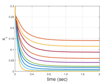
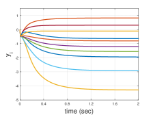
To implement the MD method, we employ the negative entropy function ϕi(xi)=k=1nxi,klog(xi,k)\phi_{i}(x_{i})\!=\!\sum_{k=1}^{n}x_{i,k}\!\log(x_{i,k}) as the generating function on Ωi\Omega_{i} in Algorithm 1. In Fig. 1, we show the trajectories of one dimension of each xix_{i} and yiy_{i}, respectively. Clearly, the trajectories of both xix_{i} and yiy_{i} in MDBD are bounded, while the boundedness of yiy_{i} may not be guaranteed in [14, 19].

Refer to caption
(a) Trajectories of xix_{i}
Refer to caption
(b) Trajectories of yiy_{i}
Figure 1: Trajectories of all agents’ variables.

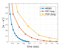
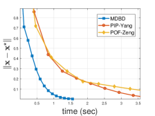
Next, we show the effectiveness of MDBD by comparisons. As is investigated in [16, 14], when the generating function satisfies ϕi(xi)=k=1nxi,klog(xi,k)\phi_{i}(x_{i})\!=\!\sum_{k=1}^{n}x_{i,k}\!\log(x_{i,k}) on the unit simplex, ΠΩiϕi(yi)\Pi_{\Omega_{i}}^{\phi_{i}}(y_{i}) can be explicitly expressed as (5). In this circumstance, the MD-based method works better than projection-based algorithms, since it can be regarded as projection-free and effectively saves the time for projection operation, especially with high-dimensional variables.

To this end, we investigate different dimensions of decision variable xix_{i} and compare MDBD with two distributed continuous-time projection-based algorithms — the proportional-integral protocol (PIP-Yang) in [8] and the projected output feedback (POF-Zeng) in [23], still for the cost functions and the coupled constraints given in (19).

TABLE I: Real running time (sec) in different dimensions
n=4n=4 n=64n=64 n=256n=256 n=1024n=1024 n=4096n=4096 n=105n=10^{5} n=106n=10^{6}
MDBD 0.47 2.42 6.76 12.98 27.99 146.62 466.60
PIP-YANG 2.51 19.63 48.51 195.67 892.74 >3000>3000 >5000>5000
POF-ZENG 3.92 21.78 39.73 207.03 1136.85 >3000>3000 >5000>5000

In Fig. 2, the xx-axis is for the real running time of the GPU, while the yy-axis is for the optimal error 𝒙𝒙\|\bm{x}-\bm{x}^{\star}\|. As the dimension increases, the real running time of the two projection-based dynamics is obviously longer than that of MDBD, because obtaining (5) is much faster than calculating a projection on high-dimensional constraint sets via solving a general quadratic optimization problem.

Refer to caption
(a) n=4n=4
Refer to caption
(b) n=16n=16
Refer to caption
(c) n=64n=64
Refer to caption
(d) n=256n=256
Figure 2: Optimal errors in different dimensions: n=4,16,64,256n=4,16,64,256.

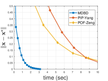
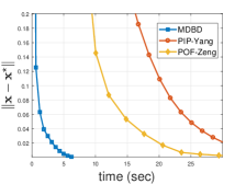
Furthermore, Table I lists the real running time for three algorithms with different dimensions of decision variables. As the dimension increases, finding the projection points in large-scale circumstances becomes more and more difficult. But remarkably, MDBD still maintains good performance, due to the advantage of MD.

VI CONCLUSIONS

We investigated distributed nonsmooth optimization with both local set constraints and coupled constraints. Based on the mirror descent method, we proposed a continuous-time algorithm with introducing the Bregman damping to guarantee the algorithm’s boundedness and accuracy. Furthermore, we utilized nonsmooth techniques, conjugate functions, and the Lyapunov stability to prove the convergence. Finally, we implemented comparative experiments to illustrate the effectiveness of our algorithm.

References

  • [1] T. Yang, X. Yi, J. Wu, Y. Yuan, D. Wu, Z. Meng, Y. Hong, H. Wang, Z. Lin, and K. H. Johansson, “A survey of distributed optimization,” Annual Reviews in Control, vol. 47, pp. 278–305, 2019.
  • [2] M. Zhu and S. Martínez, “On distributed convex optimization under inequality and equality constraints,” IEEE Transactions on Automatic Control, vol. 57, no. 1, pp. 151–164, 2011.
  • [3] D. Yuan, D. W. Ho, and S. Xu, “Regularized primal–dual subgradient method for distributed constrained optimization,” IEEE Transactions on Cybernetics, vol. 46, no. 9, pp. 2109–2118, 2015.
  • [4] A. Cherukuri and J. Cortes, “Initialization-free distributed coordination for economic dispatch under varying loads and generator commitment,” Automatica, vol. 74, pp. 183–193, 2016.
  • [5] J.-M. Xu and Y. C. Soh, “A distributed simultaneous perturbation approach for large-scale dynamic optimization problems,” Automatica, vol. 72, pp. 194–204, 2016.
  • [6] K. You, R. Tempo, and P. Xie, “Distributed algorithms for robust convex optimization via the scenario approach,” IEEE Transactions on Automatic Control, vol. 64, no. 3, pp. 880–895, 2018.
  • [7] K. Lu, G. Jing, and L. Wang, “Online distributed optimization with strongly pseudoconvex-sum cost functions,” IEEE Transactions on Automatic Control, vol. 65, no. 1, pp. 426–433, 2019.
  • [8] S. Yang, Q. Liu, and J. Wang, “A multi-agent system with a proportional-integral protocol for distributed constrained optimization,” IEEE Transactions on Automatic Control, vol. 62, no. 7, pp. 3461–3467, 2016.
  • [9] Y. Zhu, W. Yu, G. Wen, G. Chen, and W. Ren, “Continuous-time distributed subgradient algorithm for convex optimization with general constraints,” IEEE Transactions on Automatic Control, vol. 64, no. 4, pp. 1694–1701, 2018.
  • [10] S. Liang, X. Zeng, and Y. Hong, “Distributed nonsmooth optimization with coupled inequality constraints via modified Lagrangian function,” IEEE Transactions on Automatic Control, vol. 63, no. 6, pp. 1753–1759, 2017.
  • [11] X. Li, L. Xie, and Y. Hong, “Distributed continuous-time nonsmooth convex optimization with coupled inequality constraints,” IEEE Transactions on Control of Network Systems, vol. 7, no. 1, pp. 74–84, 2019.
  • [12] W. Li, X. Zeng, S. Liang, and Y. Hong, “Exponentially convergent algorithm design for constrained distributed optimization via non-smooth approach,” IEEE Transactions on Automatic Control, 2021, doi: 10.1109/TAC.2021.3075666.
  • [13] A. S. Nemirovskij and D. B. Yudin, Problem Complexity and Method Efficiency in Optimization.   Wiley-Interscience, 1983.
  • [14] W. Krichene, A. Bayen, and P. Bartlett, “Accelerated mirror descent in continuous and discrete time,” in Advances in Neural Information Processing Systems, vol. 28, 2015, pp. 2845–2853.
  • [15] J. Diakonikolas and L. Orecchia, “The approximate duality gap technique: A unified theory of first-order methods,” SIAM Journal on Optimization, vol. 29, no. 1, pp. 660–689, 2019.
  • [16] A. Ben-Tal, T. Margalit, and A. Nemirovski, “The ordered subsets mirror descent optimization method with applications to tomography,” SIAM Journal on Optimization, vol. 12, no. 1, pp. 79–108, 2001.
  • [17] S. Shahrampour and A. Jadbabaie, “Distributed online optimization in dynamic environments using mirror descent,” IEEE Transactions on Automatic Control, vol. 63, no. 3, pp. 714–725, 2017.
  • [18] D. Yuan, Y. Hong, D. W. Ho, and G. Jiang, “Optimal distributed stochastic mirror descent for strongly convex optimization,” Automatica, vol. 90, pp. 196–203, 2018.
  • [19] Y. Sun and S. Shahrampour, “Distributed mirror descent with integral feedback: Asymptotic convergence analysis of continuous-time dynamics,” IEEE Control Systems Letters, vol. 5, no. 5, pp. 1507–1512, 2020.
  • [20] Y. Wang, Z. Tu, and H. Qin, “Distributed stochastic mirror descent algorithm for resource allocation problem,” Control Theory and Technology, vol. 18, no. 4, pp. 339–347, 2020.
  • [21] P. Xu, T. Wang, and Q. Gu, “Continuous and discrete-time accelerated stochastic mirror descent for strongly convex functions,” in International Conference on Machine Learning, 2018, pp. 5492–5501.
  • [22] B. Gao and L. Pavel, “Continuous-time discounted mirror-descent dynamics in monotone concave games,” IEEE Transactions on Automatic Control, 2020, doi: 10.1109/TAC.2020.3045094.
  • [23] X. Zeng, P. Yi, Y. Hong, and L. Xie, “Distributed continuous-time algorithms for nonsmooth extended monotropic optimization problems,” SIAM Journal on Control and Optimization, vol. 56, no. 6, pp. 3973–3993, 2018.
  • [24] S. Boyd and L. Vandenberghe, Convex Optimization.   Cambridge University Press, 2004.
  • [25] J. Cortés, “Discontinuous dynamical systems,” IEEE Control Systems Magazine, vol. 28, no. 3, pp. 36–73, 2008.
  • [26] G. Shi and K. H. Johansson, “Randomized optimal consensus of multi-agent systems,” Automatica, vol. 48, no. 12, pp. 3018–3030, 2012.
  • [27] P. Yi, Y. Hong, and F. Liu, “Initialization-free distributed algorithms for optimal resource allocation with feasibility constraints and application to economic dispatch of power systems,” Automatica, vol. 74, pp. 259–269, 2016.
  • [28] G. Chen, Y. Ming, Y. Hong, and P. Yi, “Distributed algorithm for ε\varepsilon-generalized nash equilibria with uncertain coupled constraints,” Automatica, vol. 123, p. 109313, 2021.
  • [29] W. M. Haddad and V. Chellaboina, Nonlinear Dynamical Systems and Control: A Lyapunov-based Approach.   Princeton University Press, 2011.