^†^†thanks: This work was presented in part at IEEE International Symposium on Information Theory (ISIT) 2021.

Distributed Quantum Faithful Simulation and Function Computation Using Algebraic Structured Measurements

Touheed Anwar Atif and S. Sandeep Pradhan University of Michigan, Ann Arbor
touheed@umich.edu, pradhanv@umich.edu

Abstract

In this work, we consider the task of faithfully simulating a quantum measurement, acting on a joint bipartite quantum state, in a distributed manner. In the distributed setup, the constituent sub-systems of the joint quantum state are measured by two agents, Alice and Bob. A third agent, Charlie receives the measurement outcomes sent by Alice and Bob. Charlie uses local and pairwise shared randomness to compute a bivariate function of the measurement outcomes. The objective of three agents is to faithfully simulate the given distributed quantum measurement acting on the given quantum state while minimizing the communication and shared randomness rates. We demonstrate a new achievable quantum information-theoretic rate-region that exploits the bivariate function using random structured POVMs based on asymptotically good algebraic codes. The algebraic structure of these codes is matched to that of the bivariate function that models the action of Charlie. The conventional approach for this class of problems has been to reconstruct individual measurement outcomes corresponding to Alice and Bob, at Charlie, and then compute the bivariate function. This is achieved using mutually independent approximating POVMs based on random unstructured codes. In the present approach, using algebraic structured POVMs, the computation is performed on the fly, thus obviating the need to reconstruct individual measurement outcomes at Charlie. Using this, we show that a strictly larger rate region can be achieved. The performance limit is characterized using single-letter quantum mutual information quantities. We provide examples to illustrate the information-theoretic gains attained by endowing POVMs with algebraic structure. One of the challenges in analyzing these structured POVMs is that they exhibit only pairwise independence and induce only uniform single-letter distributions. To address this, we use nesting of algebraic codes and develop a covering lemma applicable to pairwise-independent POVM ensembles. Combining these techniques, we provide a multi-party distributed faithful simulation and function computation protocol.

^†^†preprint: APS/123-QED

I Introduction

Measurement compression is one of the foremost and fundamental quantum information processing techniques which form the basis of many quantum protocols [1]. One of the seminal works in this regard was by Winter [2], where he performed a novel information theoretic analysis to compress measurements in an asymptotic sense. The measurement compression problem formulated in [2] is as follows. Consider an agent (Alice) who performs a measurement $M$ on a quantum state $\rho$ , and sends a set of classical bits to another agent (Bob). Bob intends to faithfully recover the outcomes of Alice’s measurements without having access to $\rho$ , while preserving the correlation with the post-measured state of Alice’s reference. The major contribution of this work (as elaborated in [3]) was in specifying an optimal rate region in terms of classical communication and common randomness needed to faithfully simulate the action of repeated independent measurements performed on many independent copies of the given quantum state.

Wilde et al. [3] extended the measurement compression problem by considering additional resources available to each of the participating parties. One such formulation allows Bob to process the information received from Alice using local private randomness. The authors here also combined the ideas from [2] and [4] to simulate a measurement in presence of quantum side information. In the above problem formulations, authors have derived the results using the prevalent random coding techniques analogous to Shannon’s unstructured random codes [5] involving mutually independent codewords. The point-to-point setup [2, 3] requires randomly generating approximating POVMs and analyzing the error associated with these approximating POVMs, also termed as “covering error”. The key analytical tool that facilitates this is the operator Chernoff bound [6], which crucially exploits the mutual independence of codewords, yielding the quantum covering lemma [7, Lemma 17.2.1].

The measurement compression problem has been studied extensively. Early works on quantifying the information gain of a measurement include [8, 9, 10]. Buscemi et al. [11, 12, 13] later advocated quantum mutual information with respect to a classical-quantum state as the measure to characterize the corresponding information gain. Berta et al. [14] generalized the Winter’s measurement compression theorem by developing a universal measurement compression theorem for arbitrary inputs, and identified the quantum mutual information of a measurement as the information gained by performing the measurement, independent of the input state on which it is performed. They provide a proof based on new “classically coherent state merging protocol” - a variation of the quantum state merging protocol [15, 16], and the post-selection technique for quantum channels [17].

Anshu et al. [18] considered the problem of measurement compression with side information in the one-shot setting. They presented a protocol by proposing a new convex-split lemma for classical-quantum states and employing the position based decoding, and bounded the communication in terms of smooth max and hypothesis testing relative entropies. The original convex-split lemma [19, 20] demanded sub-optimal shared-randomness rate in the one-shot setting, by requiring large amount of additional quantum states in its statement. The authors addressed this by modifying the lemma to only use pairwise independent random variables. This substantially simplified the derandomization required, leading to an exponential reduction in the randomness cost in comparison to [19]. Considering a related problem, Renes and Renner [21] also studied sending of classical messages in the presence of quantum side information in the one-shot setting. For more discussion and results pertaining to one-shot quantum information theory, the reader is directed to [22, 23].

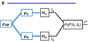
Furthermore, the authors in [24] considered the task of quantifying “relevant information” for the quantum measurements performed in a distributed fashion on bipartite entangled states involving three agents. In this multi-terminal setting, a composite bipartite quantum system $AB$ is made available to two agents, Alice and Bob, where they have access to the sub-systems $A$ and $B$ , respectively. Two separate measurements, one for each sub-system, are performed in a distributed fashion with no communication taking place between Alice and Bob. A third party, Charlie, is connected to Alice and Bob via two separate classical links. The objective of the three parties is to simulate the action of repeated independent measurements performed on many independent copies of the given composite state. Further, common randomness at rate $C$ is also shared amidst the three parties. This is achieved using random unstructured code ensembles while still using the operator Chernoff bound.

The measurement compression theorem has found its applications in several quantum information processing protocols. Examples include the quantum reverse Shannon theorem [25, 26, 27], local purity distillation protocols [28, 29, 30, 31], and also in the grandmother protocol [1] which is useful in entanglement distillation from noisy quantum states.

An ubiquitous application of distributed systems in current quantum settings arises due to the inherent vulnerability of the large-scale quantum computation systems to noise. The state-of-art systems exhibits technical difficulties in increasing the number of low-noise qubits in a single quantum device. A solution to this is cooperative processing of information separately on spatially segregated units. This necessitates the need for distributed compression protocols to compress efficiently and recover the data. In addition, when one is interested in solely reconstructing functions of the distributively stored quantum data, the rate of communication may be further reduced by employing structured coding techniques. For this, we need to impose further structure on these POVMs. This is to ensure that the joint decoder (Charlie) is able to reconstruct a lower dimensional quantum state with minimal use of the classical communication resource. Hence, structure of the POVM is desired to match with the structure of the function being computed.

The traditional random coding techniques using unstructured code ensembles may not always achieve optimality for distributed multi-terminal settings. For instance, the work by Korner-Marton [32] demonstrated this sub-optimality for the problem of classical distributed lossless compression with the objective of computing the sum of the sources for the binary symmetric case using random linear codes. Traditionally, algebraic-structured codes are used in information coding problems toward achieving computationally efficient (polynomial-time) encoding and decoding algorithms. However, in multi-terminal communication problems, even if computational complexity is a non-issue, random algebraic structured codes outperform random unstructured codes in terms of achieving improved asymptotic rate regions in many cases [33, 34, 35, 36].

Motivated by this, we consider the quantum distributed faithful measurement simulation problem and present a new achievable rate-region using algebraic structured coding techniques. However, there are two main challenges in using these algebraic structured codes toward an asymptotic analysis in quantum information theory. The first challenge is to be able to induce arbitrary empirical single-letter distributions. For example, if we were to send codewords from a linear code with uniform probability, then the induced empirical distribution of codeword symbols (single-letter distribution on the symbols of the codewords) is uniform. To address this challenge, we use a collection of cosets of a linear code called Unionized Coset Codes (UCCs) [37]. The second challenge is that unlike the random unstructured codes, the codewords generated from a random linear code are only pairwise-independent [38]. This renders the above technique of operator Chernoff bound, or even the covering lemma, unusable. Since our approach relies on the use of UCCs for generating the approximating POVMs, the binning of these POVM elements is performed in a correlated fashion as governed by these structured codes. This is in contrast to the common technique of independent binning. Due to the correlated binning, the pairwise-independence issue gets exacerbated.

We address these challenges using three main ideas summarized as follows:

•

Random structured generation of pruned POVMs - We generate a collection of algebraic structured approximating POVMs randomly using the above described UCC technique, and then prune them. This pruning ensures that these POVMs form a positive resolution of identity, and thus eliminates any need for the operator Chernoff inequality. However, such pruning comes at the cost of additional approximating error. To bound the approximating error caused by pruning the POVMs, we develop a new Operator Inequality which provides a handle to convert the pruning error in the form of covering error expression (dealt within the next idea).
•

Covering Lemma for Pairwise-Independent Ensemble - Since the traditional covering lemma is based on the Chernoff inequality, we develop an alternative proof for the aforementioned covering lemma [39, Lemma 17.2.1]. This alternative proof is based on the second-order analysis using the operator trace inequalities and hence requires the operators to be only pairwise-independent.
•

Multi-partite Packing Lemma - We develop a binning technique for performing computation on the fly so as to achieve a low dimensional reconstruction of a function at the location of Charlie. In an effort towards analysing this binning technique, we develop a multi-partite packing Lemma for the structured POVMs.

Combining these techniques, we provide a multi-party distributed faithful simulation and function computation protocol in a quantum information theoretic setting. We provide a characterization of the asymptotic performance limit of this protocol in terms of a computable single-letter achievable rate-region, which is the main result of the paper (see Theorem 1).

The organization of the paper is as follows. In Section II, we set the notation, state requisite definitions and also provide related results. In Section III.1 we state our main result on the distributed measurement compression and provide the theorem (Theorem 1) characterizing the rate-region. In Section III.2 we provide a new Covering Lemma for pairwise-independent ensembles. Section IV provides useful lemmas. In Section V, we consider the point-to-point setup and provide a theorem characterizing the rate-region using algebraic structured codes. We prove the main result (Theorem 1) in Section VI using the point-to-point result as a building block. Finally, we conclude the paper in Section VII.

II Preliminaries

Notation: Given any natural number $M$ , let the finite set $\{1,2,\cdots,M\}$ be denoted by $[1,M]$ . Let $\mathcal{B(H)}$ denote the algebra of all bounded linear operators acting on a finite dimensional Hilbert space $\mathcal{H}$ . Further, let $\mathcal{D(H)}$ denote the set of all unit trace positive operators acting on $\mathcal{H}$ . Let $I$ denote the identity operator. The trace distance between two operators $A$ and $B$ is defined as $\|A-B\|_{1}\mathrel{\ensurestackMath{\stackon[1pt]{=}{\scriptstyle\Delta}}}\Tr|A-B|$ , where for any operator $\Lambda$ we define $|\Lambda|\mathrel{\ensurestackMath{\stackon[1pt]{=}{\scriptstyle\Delta}}}\sqrt{\Lambda^{\dagger}\Lambda}$ . The von Neumann entropy of a density operator $\rho\in\mathcal{D}(\mathcal{H})$ is denoted by $S(\rho)$ . The quantum mutual information for a bipartite density operator $\rho_{AB}\in\mathcal{D}(\mathcal{H}_{A}\otimes\mathcal{H}_{B})$ is defined as

\displaystyle I(A;B)_{\rho}

\displaystyle\mathrel{\ensurestackMath{\stackon[1pt]{=}{\scriptstyle\Delta}}}S(\rho_{A})+S(\rho_{B})-S(\rho_{AB}).

A positive-operator valued measure (POVM) acting on a Hilbert space $\mathcal{H}$ is a collection $M\mathrel{\ensurestackMath{\stackon[1pt]{=}{\scriptstyle\Delta}}}\{\Lambda_{x}\}_{x\in\mathcal{X}}$ of positive operators in $\mathcal{B}(\mathcal{H})$ that form a resolution of the identity:

\displaystyle\Lambda_{x}\geq 0,\forall x\in\mathcal{X},\qquad\sum_{x\in\mathcal{X}}\Lambda_{x}=I,

where $\mathcal{X}$ is a finite set. If instead of the equality above, the inequality $\sum_{x}\Lambda_{x}\leq I$ holds, then the collection is said to be a sub-POVM. A sub-POVM $M$ can be completed to form a POVM, denoted by $[M]$ , by adding the operator $\Lambda_{0}\mathrel{\ensurestackMath{\stackon[1pt]{=}{\scriptstyle\Delta}}}(I-\sum_{x}\Lambda_{x})$ to the collection. Let $\Psi^{\rho}_{RA}$ denote a purification of a density operator $\rho\in D(\mathcal{H}_{A})$ . Given a POVM $M\mathrel{\ensurestackMath{\stackon[1pt]{=}{\scriptstyle\Delta}}}\{\Lambda^{A}_{x}\}_{x\in\mathcal{X}}$ acting on $\rho$ , the post-measurement state of the reference together with the classical outputs is represented by

(\text{id}\otimes M)(\Psi^{\rho}_{RA})\mathrel{\ensurestackMath{\stackon[1pt]{=}{\scriptstyle\Delta}}}\sum_{x\in\mathcal{X}}\outerproduct{x}{x}\otimes\Tr_{A}\{(I^{R}\otimes\Lambda_{x}^{A})\Psi^{\rho}_{RA}\}.

(1)

Consider two POVMs $M_{A}=\{\Lambda^{A}_{x}\}_{x\in\mathcal{X}}$ and $M_{B}=\{\Lambda^{B}_{y}\}_{y\in\mathcal{Y}}$ acting on $\mathcal{H}_{A}$ and $\mathcal{H}_{B}$ , respectively. Define $M_{A}\otimes M_{B}\mathrel{\ensurestackMath{\stackon[1pt]{=}{\scriptstyle\Delta}}}\{\Lambda^{A}_{x}\otimes\Lambda^{B}_{y}\}_{x\in\mathcal{X},y\in\mathcal{Y}}$ With this definition, $M_{A}\otimes M_{B}$ is a POVM acting on $\mathcal{H}_{A}\otimes\mathcal{H}_{B}$ . By $M^{\otimes n}$ denote the $n$ -fold tensor product of the POVM $M$ with itself. For a prime $p$ , we denote the unique finite field of size $p$ by $\mathbb{F}_{p}$ , and denote the addition operation over the field by $+$ .

Definition 1 (Faithful simulation [3]).

Given a POVM ${M}\mathrel{\ensurestackMath{\stackon[1pt]{=}{\scriptstyle\Delta}}}\{\Lambda_{x}\}_{x\in\mathcal{X}}$ acting on a Hilbert space $\mathcal{H}$ and a density operator $\rho\in\mathcal{D}(\mathcal{H})$ , a sub-POVM $\tilde{M}\mathrel{\ensurestackMath{\stackon[1pt]{=}{\scriptstyle\Delta}}}\{\tilde{\Lambda}_{x}\}_{x\in\mathcal{X}}$ acting on $\mathcal{H}$ is said to be $\epsilon$ -faithful to $M$ with respect to $\rho$ , for $\epsilon>0$ , if the following holds:

\sum_{x\in\mathcal{X}}\Big{\|}\sqrt{\rho}(\Lambda_{x}-\tilde{\Lambda}_{x})\sqrt{\rho}\Big{\|}_{1}+\Tr\left\{(I-\sum_{x}\tilde{\Lambda}_{x})\rho\right\}\leq\epsilon.

(2)

Lemma 1.

Given a density operator $\rho_{AB}\in\mathcal{D}(\mathcal{H}_{A}\otimes\mathcal{H}_{B})$ , a sub-POVM $M_{Y}\mathrel{\ensurestackMath{\stackon[1pt]{=}{\scriptstyle\Delta}}}\left\{\Lambda_{y}^{B}:y\in\mathcal{Y}\right\}$ acting on $\mathcal{H}_{B},$ for some set $\mathcal{Y}$ , and any Hermitian operator $\Gamma^{A}$ acting on $\mathcal{H}_{A}$ , we have

\displaystyle\sum_{y\in\mathcal{Y}}\left\|\sqrt{\rho_{AB}}\left(\Gamma^{A}\otimes\Lambda_{y}^{B}\right)\sqrt{\rho_{AB}}\right\|_{1}\leq\left\|\sqrt{\rho_{A}}\Gamma^{A}\sqrt{\rho_{A}}\right\|_{1},

(3)

with equality if $\displaystyle\sum_{y\in\mathcal{Y}}\Lambda_{y}^{B}=I$ , where $\rho_{A}=\Tr_{B}\{\rho_{AB}\}$ .

Proof.

The proof is provided in Lemma 3 of [24]. ∎

III Main Results

In this section we present the main results of this paper.

III.1 Simulation of Distributed POVMs using Algebraic-Structured POVMs

Let $\rho_{AB}$ be a density operator acting on a composite Hilbert Space $\mathcal{H}_{A}\otimes\mathcal{H}_{B}$ . Consider two measurements $M_{A}$ and $M_{B}$ on sub-systems $A$ and $B$ , respectively. Imagine again that we have three parties, named Alice, Bob and Charlie, that are trying to collectively simulate the action of a given measurement $M_{AB}$ performed on the state $\rho_{AB}$ , as shown in Fig. 1. Charlie additionally has access to unlimited private randomness. The problem is defined in the following.

Refer to caption — Figure 1: The diagram depicting the distributed POVM simulation problem with stochastic processing. In this setting, Charlie additionally has access to unlimited private randomness.

Definition 2.

For a given finite set $\mathcal{Z}$ , and a Hilbert space $\mathcal{H}_{A}\otimes\mathcal{H}_{B}$ , a distributed protocol with stochastic processing with parameters $(n,\Theta_{1},\Theta_{2},N_{1},N_{2})$ is characterized by
1) a collections of Alice’s sub-POVMs $\tilde{M}_{A}^{(\mu_{1})},\mu_{1}\in[1,N_{1}]$ each acting on $\mathcal{H}_{A}^{\otimes n}$ and with outcomes in a subset $\mathcal{L}_{1}$ satisfying $|\mathcal{L}_{1}|\leq\Theta_{1}$ .
2) a collections of Bob’s sub-POVMs $\tilde{M}_{B}^{(\mu_{2})},\mu_{2}\in[1,N_{2}]$ each acting on $\mathcal{H}_{B}^{\otimes n}$ and with outcomes in a subset $\mathcal{L}_{2}$ , satisfying $|\mathcal{L}_{2}|\leq\Theta_{2}$ .
3) a collection of Charlie’s classical stochastic maps $P^{(\mu_{1},\mu_{2})}(z^{n}|l_{1},l_{2})$ for all $l_{1}\in\mathcal{L}_{1},l_{2}\in\mathcal{L}_{2},z^{n}\in\mathcal{Z}^{n}$ , $\mu_{1}\in[1,N_{1}]$ and $\mu_{2}\in[1,N_{2}]$ .
The overall sub-POVM of this distributed protocol, given by $\tilde{M}_{AB}$ , is characterized by the following operators:

	$\displaystyle\tilde{\Lambda}_{z^{n}}\mathrel{\ensurestackMath{\stackon[1pt]{=}{\scriptstyle\Delta}}}\frac{1}{N_{1}}\frac{1}{N_{2}}\sum_{\mu_{1},\mu_{2}}$	$\displaystyle\sum_{l_{1},l_{2}}P^{(\mu_{1},\mu_{2})}(z^{n}\|l_{1},l_{2})$
		$\displaystyle\Lambda^{A,(\mu_{1})}_{l_{1}}\otimes\Lambda^{B,(\mu_{2})}_{l_{2}},\quad\forall z^{n}\in\mathcal{Z}^{n},$

where $\Lambda^{A,(\mu_{1})}_{l_{1}}$ and $\Lambda^{B,(\mu_{2})}_{l_{2}}$ are the operators corresponding to the sub-POVMs $\tilde{M}_{A}^{(\mu_{1})}$ and $\tilde{M}_{B}^{(\mu_{2})}$ , respectively.

In the above definition, $(\Theta_{1},\Theta_{2})$ determines the amount of classical bits communicated from Alice and Bob to Charlie. The amount of pairwise shared randomness is determined by $N_{1}$ and $N_{2}$ . The classical stochastic maps $P^{(\mu_{1},\mu_{2})}(z^{n}|l_{1},l_{2})$ represent the action of Charlie on the received classical bits.

Definition 3.

Given a POVM $M_{AB}$ acting on $\mathcal{H}_{A}\otimes\mathcal{H}_{B}$ , and a density operator $\rho_{AB}\in\mathcal{D}(\mathcal{H}_{A}\otimes\mathcal{H}_{B})$ , a quadruple $(R_{1},R_{2},C_{1},C_{2})$ is said to be achievable, if for all $\epsilon>0$ and for all sufficiently large $n$ , there exists a distributed protocol with stochastic processing with parameters $(n,\Theta_{1},\Theta_{2},N_{1},N_{2})$ such that its overall sub-POVM $\tilde{M}_{AB}$ is $\epsilon$ -faithful to $M_{AB}^{\otimes n}$ with respect to $\rho_{AB}^{\otimes n}$ (see Definition 1), and

\displaystyle\frac{1}{n}\log_{2}\Theta_{i}\leq R_{i}+\epsilon,\!\quad\mbox{and}\!\quad\!\frac{1}{n}\log_{2}N_{i}\leq C_{i}+\epsilon,\quad i=1,2.

The set of all achievable quadruples $(R_{1},R_{2},C_{1},C_{2})$ is called the achievable rate region.

Definition 4 (Joint Measurements).

A POVM $M_{AB}=\{\Lambda^{AB}_{z}\}_{z\in\mathcal{Z}}$ , acting on a Hilbert space $\mathcal{H}_{A}\otimes\mathcal{H}_{B}$ , is said to have a separable decomposition with stochastic integration given by $(\bar{M}_{A},\bar{M}_{B},P_{Z|S,T})$ if there exist POVMs $\bar{M}_{A}=\{\bar{\Lambda}^{A}_{s}\}_{s\in\mathcal{S}}$ and $\bar{M}_{B}=\{\bar{\Lambda}^{B}_{t}\}_{t\in\mathcal{T}}$ and a stochastic mapping $P_{Z|S,T}:\mathcal{S}\times\mathcal{T}\rightarrow\mathcal{Z}$ such that

\Lambda^{AB}_{z}=\sum_{s,t}P_{Z|S,T}(z|s,t)\bar{\Lambda}^{A}_{s}\otimes\bar{\Lambda}^{B}_{t},\quad\forall z\in\mathcal{Z},

(4)

where $\mathcal{S},\mathcal{T}$ , and $\mathcal{Z}$ are finite sets.

The following theorem provides an inner bound to the achievable rate region, which is proved in Section VI. This is one of the main results of this paper.

Theorem 1.

Consider a density operator $\rho_{AB}\in\mathcal{D}(\mathcal{H}_{A}\otimes\mathcal{H}_{B})$ , and a POVM $M_{AB}=\{\Lambda^{AB}_{z}\}_{z\in\mathcal{Z}}$ acting on $\mathcal{H}_{A}\otimes\mathcal{H}_{B}$ having a separable decomposition with stochastic integration (as in Definition 4), yielding POVMs $\bar{M}_{A}=\{\bar{\Lambda}^{A}_{s}\}_{s\in\mathcal{S}}$ and $\bar{M}_{B}=\{\bar{\Lambda}^{B}_{t}\}_{t\in\mathcal{T}}$ and a stochastic map $P_{Z|S,T}:\mathcal{S}\times\mathcal{T}\rightarrow\mathcal{Z}$ . Define the auxiliary states

	$\displaystyle\sigma_{1}^{RSB}$	$\displaystyle\mathrel{\ensurestackMath{\stackon[1pt]{=}{\scriptstyle\Delta}}}(\emph{id}_{R}\otimes\bar{M}_{A}\otimes\emph{id}_{B})(\Psi^{\rho_{AB}}_{RAB}),$
	$\displaystyle\sigma_{2}^{RTV}$	$\displaystyle\mathrel{\ensurestackMath{\stackon[1pt]{=}{\scriptstyle\Delta}}}(\emph{id}_{R}\otimes\emph{\text{id}}_{A}\otimes\bar{M}_{B})(\Psi^{\rho_{AB}}_{RAB}),\quad\text{and}$
	$\displaystyle\sigma_{3}^{RSTZ}$	$\displaystyle\mathrel{\ensurestackMath{\stackon[1pt]{=}{\scriptstyle\Delta}}}\sum_{s,t,z}\sqrt{\rho_{AB}}\left(\bar{\Lambda}^{A}_{s}\otimes\bar{\Lambda}^{B}_{t}\right)\sqrt{\rho_{AB}}$
		$\displaystyle\hskip 30.0pt\otimes P_{Z\|S,T}(z\|s,t)\outerproduct{s}{s}\otimes\outerproduct{t}{t}\otimes\outerproduct{z}{z},$

for some orthonormal sets $\{\ket{s}\}_{s\in\mathcal{S}},\{\ket{t}\}_{t\in\mathcal{T}}$ , and $\{\ket{z}\}_{z\in\mathcal{Z}}$ , where $\Psi^{\rho_{AB}}_{RAB}$ is a purification of $\rho_{AB}$ . A quadruple $(R_{1},R_{2},C_{1},C_{2})$ is achievable if there exists a finite field $\mathbb{F}_{p}$ , for a prime $p$ , a pair of mappings $f_{S}:\mathcal{S}\rightarrow\mathbb{F}_{p}$ and $f_{T}:\mathcal{T}\rightarrow\mathbb{F}_{p}$ , and a stochastic mapping $P_{Z|W}:\mathbb{F}_{p}\rightarrow\mathcal{Z}$ such that

P_{Z|S,T}(z|s,t)\!=\!P_{Z|W}(z|f_{S}(s)+f_{T}(t)),\forall s\!\in\!\mathcal{S},t\!\in\!\mathcal{T},z\!\in\!\mathcal{Z},

yielding $U=f_{S}(S)$ , $V=f_{T}(T)$ , and $W=U+V$ , and the following inequalities are satisfied:


	$\displaystyle R_{1}\geq I(U;R,B)_{\sigma_{1}}+I(W;V)_{\sigma_{3}}-I(U;V)_{\sigma_{3}},$		(5a)
	$\displaystyle R_{2}\geq I(V;R,A)_{\sigma_{2}}+I(W;U)_{\sigma_{3}}-I(U;V)_{\sigma_{3}},$		(5b)
	$\displaystyle R_{1}+C_{1}\geq I(U;\!R,Z)_{\sigma_{3}}+I(W;V)_{\sigma_{3}}-I(U;V)_{\sigma_{3}},$		(5c)
	$\displaystyle R_{2}+C_{2}\geq I(V;\!R,Z)_{\sigma_{3}}+I(W;U)_{\sigma_{3}}-I(U;V)_{\sigma_{3}},$		(5d)
	$\displaystyle R_{1}+R_{2}+C_{1}+C_{2}\geq I(U,V;R,Z)_{\sigma_{3}}+I(W;U)_{\sigma_{3}}$
	$\displaystyle\hskip 101.17755pt+I(W;V)_{\sigma_{3}}-I(U;V)_{\sigma_{3}}.$		(5e)

Proof.

A proof is provided in Section VI. ∎

Remark 1.

Note that the rate-region obtained in Theorem 6 of [24] using unstructured random code ensembles, contains the constraint $R_{1}+R_{2}+C_{1}+C_{2}\geq I(U,V;R,Z)_{\sigma_{3}}$ . Hence when

	$\displaystyle I(W;U)_{\sigma_{3}}$	$\displaystyle+I(W;V)_{\sigma_{3}}-I(U;V)_{\sigma_{3}}$
		$\displaystyle=2S(U+V)_{\sigma_{3}}-S(U,V)_{\sigma_{3}}<0,$

the above theorem gives a lower sum rate constraint. As a result, the rate-region above contains points that are not contained within the rate-region provided in [24]. To illustrate this fact further, consider the following example.

Remark 2.

In the above theorem, we restrict our attention to prime finite fields for ease of exposition. The results can be generalized to arbitrary finite fields in a straight-forward manner.

Example 1.

Suppose the composite state $\rho_{AB}$ is described using one of the Bell states on $\mathcal{H}_{A}\otimes\mathcal{H}_{B}$ as

\displaystyle\rho_{AB}=\cfrac{1}{2}\left(\ket{00}_{AB}+\ket{11}_{AB}\right)\left(\bra{00}_{AB}+\bra{11}_{AB}\right).

Since $\pi^{A}=\Tr_{B}{\rho^{AB}}$ and $\pi^{B}=\Tr_{A}{\rho^{AB}}$ , Alice and Bob would perceive each of their particles in maximally mixed states $\pi^{A}=\frac{I_{A}}{2}$ and $\pi^{B}=\frac{I_{B}}{2}$ , respectively. Upon receiving the quantum state, the two parties wish to independently measure their states, using identical POVMs $\bar{M}_{A}$ and $\bar{M}_{B}$ , given by $\bar{M}_{A}\mathrel{\ensurestackMath{\stackon[1pt]{=}{\scriptstyle\Delta}}}\left\{\bar{\Lambda}_{s}^{A}\right\}_{s\in\mathcal{S}},\bar{M}_{B}\mathrel{\ensurestackMath{\stackon[1pt]{=}{\scriptstyle\Delta}}}\left\{\bar{\Lambda}_{v}^{B}\right\}_{t\in\mathcal{T}}$ , where $\mathcal{S}=\mathcal{T}=\{0,1\}$ , and

	$\displaystyle\Lambda_{0}^{A}$	$\displaystyle=\Lambda_{0}^{B}\mathrel{\ensurestackMath{\stackon[1pt]{=}{\scriptstyle\Delta}}}\begin{bmatrix}0.9501&0.0826+i0.1089\\ 0.0826-i0.1089&0.0615\end{bmatrix},$
	$\displaystyle\Lambda_{1}^{A}$	$\displaystyle=\Lambda_{1}^{B}\mathrel{\ensurestackMath{\stackon[1pt]{=}{\scriptstyle\Delta}}}\begin{bmatrix}0.0499&-0.0826-i0.1089\\ -0.0826+i0.1089&0.9385\end{bmatrix}.$

Alice and Bob together with Charlie are trying to simulate the action of $M_{AB}\mathrel{\ensurestackMath{\stackon[1pt]{=}{\scriptstyle\Delta}}}\left\{\Gamma_{z}^{AB}\right\}_{z\in\mathcal{Z}}$ , using the classical communication and common randomness as the resources available to them, where $\mathcal{Z}=\{0,1\}$ , and

\displaystyle\Gamma_{z}^{AB}\mathrel{\ensurestackMath{\stackon[1pt]{=}{\scriptstyle\Delta}}}\sum_{s\in\{0,1\}}\sum_{t\in\{0,1\}}P_{Z|S,T}(z|s,t)\left(\Lambda_{s}^{A}\otimes\Lambda_{t}^{B}\right),

(6)

for $z\in\{0,1\},$ and $P_{Z|S,T}(0|0,0)=P_{Z|S,T}(0|1,1)=1-P_{Z|S,T}(0|0,1)=1-P_{Z|S,T}(0|1,0)=\lambda$ , with $\lambda\in(0,1)$ . Note that the above POVM $M_{AB}$ admits a separable decomposition as defined in the statement of Theorem 1 with respect to the prime finite field $\mathbb{F}_{2}$ , with $U=S$ and $V=T$ , and

P_{Z|W}(0|0)=1-P_{Z|W}(0|1)=\lambda.

Hence the above theorem can be employed. This gives

	$\displaystyle S(U+V)_{\sigma_{3}}$	$\displaystyle=0.5155,\quad S(U)_{\sigma_{3}}=S(V)_{\sigma_{3}}=0.9999,$
	$\displaystyle S(U,V)_{\sigma_{3}}$	$\displaystyle=1.5154,\quad I(U,V)_{\sigma_{3}}=0.4844,$

where $\sigma_{3}$ is as defined in the statement of Theorem 1. Since $S(U)_{\sigma_{3}}-S(U+V)_{\sigma_{3}}=S(V)_{\sigma_{3}}-S(U+V)_{\sigma_{3}}=I(U,V)_{\sigma_{3}},$ the constraints on $R_{1}$ , $R_{2}$ , $R_{1}+C$ and $R_{2}+C$ are the same as obtained in Theorem 6 of [24]. However, with $2S(U+V)_{\sigma_{3}}-S(U,V)_{\sigma_{3}}=-0.4844<0$ , the constraint on $R_{1}+R_{2}+C_{1}+C_{2}$ in the above theorem (5e) is strictly weaker than the constraint obtained using random unstructured codes in Theorem 6 of [24]. Therefore, the rate-region obtained above using random structured codes in Theorem 1 is strictly larger than the rate-region in Theorem 6 of [24].

Example 2.

For the same state $\rho_{AB}$ as in the above example, consider the following identical POVMs $M_{A}\mathrel{\ensurestackMath{\stackon[1pt]{=}{\scriptstyle\Delta}}}\left\{\bar{\Lambda}_{s}^{A}\right\}_{s\in\mathcal{S}}$ and $M_{B}\mathrel{\ensurestackMath{\stackon[1pt]{=}{\scriptstyle\Delta}}}\left\{\bar{\Lambda}_{t}^{B}\right\}_{t\in\mathcal{T}}$ , where $\mathcal{S}=\mathcal{T}=\{0,1\}$ , and

	$\displaystyle\Lambda_{0}^{A}$	$\displaystyle=\Lambda_{0}^{B}=\begin{bmatrix}0.4974&0.0471+i0.4975\\ 0.0471-i0.4975&0.5026\end{bmatrix},$
	$\displaystyle\Lambda_{1}^{A}$	$\displaystyle=\Lambda_{1}^{B}=\begin{bmatrix}0.5026&-0.0471-i0.4975\\ -0.0471+i0.4975&0.4974\end{bmatrix}.$

Let the joint measurement that Alice and Bob are trying to simulate be given by

\displaystyle\Gamma_{z}^{AB}\mathrel{\ensurestackMath{\stackon[1pt]{=}{\scriptstyle\Delta}}}\sum_{s\in\{0,1\}}\sum_{t\in\{0,1\}}P_{Z|S,T}(z|s,t)\left(\Lambda_{s}^{A}\otimes\Lambda_{t}^{B}\right),

(7)

for $z\in\{0,1\}$ where $P_{Z|S,T}:\{0,1\}\rightarrow[0,1]$ is a conditional PMF on $\mathcal{Z}\times\mathcal{S}\times\mathcal{T}$ with $P_{Z|S,T}(0|0,0)=\delta_{0}\in(0,1)$ and $P_{Z|S,T}(0|0,1)=P_{Z|S,T}(0|1,0)=P_{Z|S,T}(0|1,1)=\delta_{1}\in(0,1)$ . Note that $P_{Z|S,T}$ depends on the variables $(s,t)$ only through $s\lor t$ , the logical OR function. Now, we define the random variables $U$ and $V$ on the prime finite field $\mathbb{F}_{3}$ with the identity mappings $U=S$ and $V=T$ , while noting that $U$ and $V$ take values in $\mathbb{F}_{3}$ with $P(U=2)=P(V=2)=0$ . Now with $W=U+V$ , we identify the mapping $P_{Z|W}$ as

\displaystyle P_{Z|W}(0|0)=\delta_{0},\quad P_{Z|W}(0|1)=P_{Z|W}(0|2)=\delta_{1}.

(8)

For this identification, we obtain $2S(U+V)-S(U,V)=-0.9039<0$ , which gives the constraint on $R_{1}+R_{2}+C_{1}+C_{2}$ in the above theorem (5e) strictly weaker than the corresponding constraint obtained using random unstructured codes in Theorem 6 of [24]. Since this is a biting constraint, the above rate-region is strictly larger than the former for this example.

Example 3.

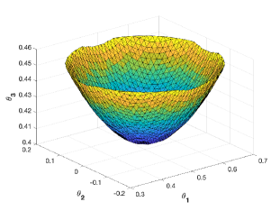
Building upon Example 2, we explore more points in the POVM space such that the above theorem provides constraints (5e) that are strictly weaker than the corresponding constraint obtained in Theorem 6 of [24]. For this, we consider the same state $\rho_{AB},$ as above and the following identical POVMs $M_{A}\mathrel{\ensurestackMath{\stackon[1pt]{=}{\scriptstyle\Delta}}}\left\{\bar{\Lambda}_{s}^{A}\right\}_{s\in\mathcal{S}}$ and $M_{B}\mathrel{\ensurestackMath{\stackon[1pt]{=}{\scriptstyle\Delta}}}\left\{\bar{\Lambda}_{t}^{B}\right\}_{t\in\mathcal{T}}$ , where $\mathcal{S}=\mathcal{T}=\{0,1\}$ , and

\displaystyle\Lambda_{0}^{A}=\Lambda_{0}^{B}=\begin{bmatrix}\theta_{1}&\theta_{2}+i\theta_{3}\\ \theta_{2}-i\theta_{3}&1-\theta_{1}\end{bmatrix},\quad\Lambda_{1}^{A}=\Lambda_{1}^{B}=I-\Lambda_{0}^{A}

for $\theta_{i}\in[-1,1]$ ¹¹1The above parametrization is only for illustrative purposes and do not constitute all the two dimensional POVMs.. Figure 2 illustrates the surface where $2S(U+V)=S(U,V)$ and therefore the region inside the surface has $2S(U+V)-S(U,V)<0$ , where the POVMs obtained provides the constraint on $R_{1}+R_{2}+C_{1}+C_{2}$ in the above theorem (5e) strictly weaker than the corresponding constraint obtained in Theorem 6 of [24].

Remark 3.

Note that for POVMs contained in the above $(\theta_{1},\theta_{2},\theta_{3})$ -surface of Example 2, the sum rate constraint $R_{1}+R_{2}+C_{1}+C_{2}$ is strictly weaker than the corresponding constraint in [24, Theorem 6], and vice-versa outside. One can employ a strategy based on superposition and successive encoding that combines the two coding techniques to yield a unified rate-region.

III.2 Covering Lemma with Change of Measure for Pairwise-Independent Ensemble

The proof of the theorem is based on a construction of algebraic-structured POVM ensemble where the elements are only pairwise independent and not mutually independent. To analyze these POVMs we retreat back to first principles and develop a new one-shot Covering Lemma based on a change of measure technique and a second order analysis. This lemma, which can be of independent interest, is one of the main contributions of this work.

Lemma 2 (Covering Lemma).

Let $\{\lambda_{x},\sigma_{x}\}_{x\in\mathcal{X}}$ be an ensemble, with $\sigma_{x}\in\mathcal{D}(\mathcal{H})$ for all $x\in\mathcal{X}$ , $\mathcal{X}$ being a finite set, and $\sigma=\sum_{x\in\mathcal{X}}\lambda_{x}\sigma_{x}$ . Further, suppose we are given a total subspace projector $\Pi$ and a collection of codeword subspace projectors $\{\Pi_{x}\}_{x\in\mathcal{X}}$ which satisfy the following hypotheses


$\displaystyle\Tr{\Pi\sigma_{x}}$	$\displaystyle\geq 1-\epsilon,$	(9a)
$\displaystyle\Tr{\Pi_{x}\sigma_{x}}$	$\displaystyle\geq 1-\epsilon,$	(9b)
$\displaystyle\\|\Pi\sqrt{\sigma}\\|^{2}_{1}$	$\displaystyle\leq D,$	(9c)
$\displaystyle\Pi_{x}\sigma_{x}\Pi_{x}$	$\displaystyle\leq\frac{1}{d}\Pi_{x},\quad\text{and}$	(9d)
$\displaystyle\Pi_{x}\sigma_{x}\Pi_{x}$	$\displaystyle\leq\sigma_{x}.$	(9e)

for some $\epsilon\in(0,1)$ and $d<D$ . Let $M$ be a finite non-negative integer. Additionally, assume that there exists some set $\bar{\mathcal{X}}$ containing $\mathcal{X}$ , with $\sigma_{x}\mathrel{\ensurestackMath{\stackon[1pt]{=}{\scriptstyle\Delta}}}0$ (null operator) and $\lambda_{x}\mathrel{\ensurestackMath{\stackon[1pt]{=}{\scriptstyle\Delta}}}0$ for $x\in\bar{\mathcal{X}}\backslash\mathcal{X}$ . Suppose $\{\mu_{\bar{x}}\}_{\bar{x}\in\bar{\mathcal{X}}}$ be any distribution on the set $\bar{\mathcal{X}}$ such that the distribution is $\{\lambda_{x}\}_{{x}\in\mathcal{X}}$ is absolutely continuous with respect to the distribution $\{\mu_{\bar{x}}\}_{\bar{x}\in\bar{\mathcal{X}}}$ . Further, assume that $\lambda_{x}/\mu_{x}\leq\kappa$ for all $x\in\mathcal{X}.$ Let a random covering code $\mathbbm{C}\mathrel{\ensurestackMath{\stackon[1pt]{=}{\scriptstyle\Delta}}}\{C_{m}\}_{m\in[1,M]}$ be defined as a collection of codewords $C_{m}$ that are chosen pairwise independently according to the distribution $\{\mu_{\bar{x}}\}_{\bar{x}\in\bar{\mathcal{X}}}$ . Then we have

\displaystyle\mathbb{E}_{\mathbbm{C}}\left[\Big{\|}\sum_{x\in\bar{\mathcal{X}}}\lambda_{x}\sigma_{x}-\frac{1}{M}\sum_{m=1}^{M}\frac{\lambda_{C_{m}}}{\mu_{C_{m}}}\sigma_{C_{m}}\Big{\|}_{1}\right]\!\leq\!\sqrt{\frac{\kappa D}{Md}}+2\delta(\epsilon),

(10)

where $\delta(\epsilon)=4\sqrt{\epsilon}$ . Futhermore, for $\tilde{\sigma}_{x}$ defined as $\tilde{\sigma}_{x}\mathrel{\ensurestackMath{\stackon[1pt]{=}{\scriptstyle\Delta}}}\Pi\Pi_{x}{\sigma}_{x}\Pi_{x}\Pi$ , we have

\displaystyle\mathbb{E}_{\mathbbm{C}}\left[\Big{\|}\sum_{x\in\bar{\mathcal{X}}}\lambda_{x}\tilde{\sigma}_{x}-\frac{1}{M}\sum_{m=1}^{M}\frac{\lambda_{C_{m}}}{\mu_{C_{m}}}\tilde{\sigma}_{C_{m}}\Big{\|}_{1}\right]\leq\sqrt{\frac{\kappa D}{Md}}.

(11)

Proof.

The proof is provided in Appendix A.1 ∎

IV Useful Lemmas

In this section we present a few lemmas which will be used extensively in the sequel.

Definition 5 (Pruning Operators).

Consider an operator $A\geq 0$ acting on Hilbert space $\mathcal{H}_{A}.$ We say that a projector $P$ prunes $A$ with respect to Identity $I_{A}$ on $\mathcal{H}_{A},$ if $P$ is a projector on to the non-negative eigenspace of $I_{A}-A$ .

IV.1 Pruning Trace Inequality

Lemma 3.

Consider a random operator $X\geq 0$ acting on a Hilbert space $\mathcal{H}_{A}.$ Let $P$ be a pruning operator for $X$ with respect to $I_{A}$ , as in Definition 5. Then we have

\mathbb{E}[\Tr{I_{A}-P}]\leq\mathbb{E}[\Tr{X}].

Proof.

The proof follows by noting that $\Tr{I_{A}-P}\leq\Tr{X}$ . ∎

Remark 4.

To demonstrate the significance of this inequality, we compare it with the popular Operator Markov Inequality [39]. We know from Operator Markov inequality

\displaystyle\mathbb{P}\left(X\nleq I_{A}\right)\leq\mathbb{E}[\Tr{X}].

One can observe that $\mathbbm{1}_{\{X\nleq I_{A}\}}\leq\Tr{I_{A}-P}$ . Taking expectation, we obtain

\displaystyle\mathbb{P}\left(X\nleq I_{A}\right)\leq\mathbb{E}[\Tr{I_{A}-P}].

Moreover, one can also note that $\Tr{I_{A}-P}\leq\Tr{X}$ , and expectation gives

\displaystyle\mathbb{E}[\Tr{I_{A}-P}]\leq\mathbb{E}[\Tr{X}].

Hence we conclude that the new inequality is indeed tighter than the operator Markov inequality.

Lemma 4.

(Pruning Trace Inequality) Consider the above random operator $X\geq 0$ acting on a Hilbert space $\mathcal{H}_{A}.$ Further, suppose $\mathbb{E}[X]\leq(1-\eta){I_{A}}$ for $\eta\in(0,1)$ . Let $P$ be a pruning operator for $X$ with respect to $I_{A}$ , as in Definition 5. Then, we have

\displaystyle\mathbb{E}[\Tr{I_{A}-P}]\leq\frac{1}{\eta}\mathbb{E}\left[\|X-\mathbb{E}[X]\|_{1}\right].

Proof.

The proof is provided in Appendix A.2 ∎

V Point-to-point Measurement Compression using Structured Random POVMs

Before presenting the proof of Theorem 1, as a pedagogical first step, we consider the measurement compression problem in the point-to-point setup. This problem was addressed in [2], where the performance limits were derived using unstructured random POVM ensembles. Here, we redrive the performance limit using random algebraic structured POVM ensembles. Since the algebraic structured codes can only induce a uniform distribution, we consider a collection of cosets of a random linear code for this task. The problem setup is described as follows. An agent (Alice) performs a measurement $M$ on a quantum state $\rho$ , and sends a set of classical bits to a receiver (Bob). Bob has access to additional private randomness, and he is allowed to use this additional resource to perform any stochastic mapping of the received classical bits. The overall effect on the quantum state can be assumed to be a measurement which is a concatenation of the POVM Alice performs and the stochastic map Bob implements. This problem serves as a building block toward the proof of Theorem 1. Formally, the problem is stated as follows.

V.1 Problem Formulation and Main Result

Definition 6.

For a given finite set $\mathcal{Z}$ , and a Hilbert space $\mathcal{H}$ , a measurement simulation protocol with parameters $(n,\Theta,N)$ is characterized by
1) a collection of codes $\mathcal{C}^{(\mu)}\subseteq\mathcal{W}^{n}$ , for $\mu\in[1,N]$ , such that $|\mathcal{C}^{(\mu)}|\leq\Theta$ , and $\mathcal{W}$ , a finite set, is called the code alphabet,
2) a collection of Alice’s sub-POVMs $\tilde{M}^{(\mu)},\mu\in[1,N]$ each acting on $\mathcal{H}^{\otimes n}$ and with outcomes in $\mathcal{C}^{(\mu)}$ .
3) a collection of Bob’s classical stochastic maps $P^{(\mu)}(z^{n}|w^{n})$ for all $w^{n}\in\mathcal{C}^{(\mu)}$ , $z^{n}\in\mathcal{Z}^{n}$ and $\mu\in[1,N]$ .
The overall sub-POVM of this protocol, given by $\tilde{M}$ , is characterized by the following operators:

\tilde{\Lambda}_{z^{n}}\mathrel{\ensurestackMath{\stackon[1pt]{=}{\scriptstyle\Delta}}}\frac{1}{N}\sum_{\mu=1}^{N}\sum_{w^{n}\in\mathcal{C}^{(\mu)}}P^{(\mu)}(z^{n}|w^{n})~{}\Lambda^{(\mu)}_{w^{n}},\quad\forall z^{n}\in\mathcal{Z}^{n},

(12)

where $\{\Lambda^{(\mu)}_{w^{n}}:w^{n}\in\mathcal{C}^{(\mu)}\}$ is the set of operators corresponding to the sub-POVM $\tilde{M}^{(\mu)}$ . Let $\mathcal{C}^{(\mu)}(i)$ denote the $i$ th codeword of $\mathcal{C}^{(\mu)}$ .

In the above definition, $\Theta$ characterizes the amount of classical bits communicated from Alice to Bob, and the amount of common randomness is determined by $N$ , with $\mu$ being the common randomness bits distributed among the parties. The classical stochastic mappings induced by $P^{(\mu)}$ represents the action of Bob on the received classical bits. In building the code, we use the Unionized Coset Code (UCC) [37] defined below. These codes involve two layers of codes (i) a coarse code and (ii) a fine code. The coarse code is a coset of the linear code and the fine code is the union of several cosets of the linear code.

For a fixed $k\times n$ matrix $G\in\mathbb{F}_{p}^{k\times n}$ with $k\leq n$ , and $p$ being a prime number, and a $1\times n$ vector $B\in\mathbb{F}_{p}^{n}$ , define the coset code as

\displaystyle\mathbb{C}(G,B)\mathrel{\ensurestackMath{\stackon[1pt]{=}{\scriptstyle\Delta}}}\{x^{n}:x^{n}=a^{k}G+B,\mbox{ for some }a^{k}\in\mathbb{F}_{p}^{k}\}.

(13)

In other words, $\mathbb{C}(G,B)$ is a shift of the row space of the matrix $G$ . The row space of $G$ is a linear code. If the rank of $G$ is $k$ , then there are $p^{k}$ codewords in the coset code.

Definition 7.

An $(n,k,l,p)$ UCC is characterized by a pair $(G,h)$ consisting of a $k\times n$ matrix $G\in\mathbb{F}_{p}^{k\times n}$ , and a mapping $h:\mathbb{F}_{p}^{l}\rightarrow\mathbb{F}_{p}^{n}$ , and the code is the following union: $\bigcup_{m\in\mathbb{F}_{p}^{l}}\mathbb{C}(G,h(m))$ , where $\mathbb{C}(\cdot,\cdot)$ is defined in (13).

Definition 8.

Given a finite set $\mathcal{Z}$ , and a Hilbert space $\mathcal{H}$ , an $(n,\Theta,\kappa,N,p)$ UCC-based measurement simulation protocol is a pair of $(n,\Theta,N)$ measurement simulation protocol and a collection of $N$ UCCs with parameters $(n,k,l,p)$ characterized by $\{(G,h^{(\mu)})\}_{\mu\in[1,N]}$ such that (i) the code alphabet of the protocol $\mathcal{W}\subseteq\mathbb{F}_{p}$ (with suitable relabeling), (ii) $\kappa=p^{k}$ , $\Theta=p^{l}$ , and (iii) for all $m\in\mathbb{F}_{p}^{l}$ , we have $\mathcal{C}^{(\mu)}(m)\in\{a^{k}G+h^{(\mu)}(m):a^{k}\in\mathbb{F}_{p}^{k}\}$ .

Definition 9.

The UCC grand ensemble is the ensemble of $N$ UCCs where $G$ , and $\{h^{(\mu)}\}_{\mu\in[1,N]}$ are chosen randomly, independently and uniformly, where the latter is chosen from the set of all mappings with replacement.

Definition 10.

Given a POVM $M$ acting on $\mathcal{H}$ , and a density operator $\rho\in\mathcal{D}(\mathcal{H})$ , a tuple $(R,R_{1},C,p)$ is said to be achievable using the grand UCC ensemble, if for all $\epsilon>0$ and for all sufficiently large $n$ , there exists an ensemble of UCC-based measurement simulation protocols with parameters $(n,\Theta,\kappa,N,p)$ (based on the UCC grand ensemble) such that their overall sub-POVM $\tilde{M}$ is $\epsilon$ -faithful to $M^{\otimes n}$ with respect to $\rho^{\otimes n}$ in the expected sense:

\displaystyle\mathbb{E}\!

\displaystyle\left[\!\sum_{z^{n}}\!\left\|\!\sqrt{\rho^{\otimes n}}(\Lambda_{z^{n}}\!-\!\tilde{\Lambda}_{z^{n}})\sqrt{\rho^{\otimes n}}\right\|\!+\!\Tr\{I-\sum_{z^{n}}\tilde{\Lambda}_{z^{n}}\}\right]\leq\epsilon,

where the expectation is with respect to the ensemble, and

\displaystyle\frac{1}{n}\log_{2}\Theta\leq R+\epsilon,\;\left|\frac{1}{n}\log\kappa-R_{1}\right|\leq\epsilon,;\;\frac{1}{n}\log_{2}N\leq C+\epsilon.

Define $\mathscr{R}_{\mbox{UCC}}$ as $\mathscr{R}_{\mbox{UCC}}\mathrel{\ensurestackMath{\stackon[1pt]{=}{\scriptstyle\Delta}}}\{(R,R_{1},C,p):(R,R_{1},C,p)$ is achievable using the UCC grand ensemble}.

Remark 5.

The appearance of the modulus in the second constraint needs justification. Note that $R$ is the rate of transmission of information from Alice to Bob and $C$ is the rate of the common information shared between them. So if $(R,R_{1},C,p)$ is achievable, then it is clear that any $(\tilde{R},\tilde{C})$ is also achievable if $\tilde{R}\geq R$ and $\tilde{C}\geq C$ . However $R_{1}$ is a parameter of the UCC grand ensemble, and there is no natural order on $R_{1}$ , i.e., it does not naturally follows that $(R,\tilde{R}_{1},C,p)$ is achievable for all $\tilde{R}_{1}\geq R_{1}$ .

The following theorem characterizes the achievable rate region which characterizes the asymptotic performance of the UCC grand ensemble.

Theorem 2.

For any density operator $\rho\in\mathcal{D}(\mathcal{H})$ and any POVM ${M}\mathrel{\ensurestackMath{\stackon[1pt]{=}{\scriptstyle\Delta}}}\{{\Lambda}_{z}\}_{z\in\mathcal{Z}}$ acting on the Hilbert space $\mathcal{H}$ , a tuple $(R,R_{1},C,p)$ is achievable using the UCC grand ensemble, i.e., $(R,R_{1},C,p)\in\mathscr{R}_{\mbox{UCC}}$ if there exist a POVM $\bar{M}\mathrel{\ensurestackMath{\stackon[1pt]{=}{\scriptstyle\Delta}}}\{\bar{\Lambda}_{w}\}_{w\in\mathcal{W}}$ , with $|\mathcal{W}|\leq p$ , and a stochastic map $P_{Z|W}:\mathcal{W}\rightarrow\mathcal{Z}$ such that

\Lambda_{z}=\sum_{w\in\mathcal{W}}P_{Z|W}(z|w)\bar{\Lambda}_{w},\quad\forall z\in\mathcal{Z},

and

$\displaystyle R_{1}+R$	$\displaystyle\geq I(W;R)_{\sigma}-S(W)_{\sigma}+\log{p},$	(14)
$\displaystyle R_{1}+R+C$	$\displaystyle\geq I(W;RZ)_{\sigma}-S(W)_{\sigma}+\log{p},$	(15)
$\displaystyle 0\leq R_{1}$	$\displaystyle\leq\log{p}-S(W)_{\sigma},$	(16)
$\displaystyle C$	$\displaystyle\geq 0,$	(17)

where $\sigma^{RWZ}\mathrel{\ensurestackMath{\stackon[1pt]{=}{\scriptstyle\Delta}}}\sum_{w,z}\sqrt{\rho}\bar{\Lambda}_{w}\sqrt{\rho}\otimes P_{Z|W}(z|w)\outerproduct{w}{w}\otimes\outerproduct{z}{z},$ for some orthogonal sets $\{\ket{w}\}_{w\in\mathcal{W}}$ and $\{\ket{z}\}_{z\in\mathcal{Z}}.$

Remark 6.

By choosing $R_{1}=\log{p}-S(W)_{\sigma}$ , we recover the rate region of Wilde et. al [3, Theorem 9].

V.2 Proof of Theorem 2 Using UCC Code Ensemble

As stated earlier, the main objective of proving this theorem is to build a framework for the main theorem of the paper (Theorem 1). In doing so, we observe that the structured POVMs constructed below are only pairwise independent. Since the results in [24] are based on the assumption that approximating POVMs are all mutually independent, the proof below becomes significantly different from [24].

Suppose there exist a POVM $\bar{M}\mathrel{\ensurestackMath{\stackon[1pt]{=}{\scriptstyle\Delta}}}\{\bar{\Lambda}_{w}\}_{w\in\mathcal{W}}$ and a stochastic map $P_{Z|W}:\mathcal{W}\rightarrow\mathcal{Z}$ , such that $M\mathrel{\ensurestackMath{\stackon[1pt]{=}{\scriptstyle\Delta}}}\{\Lambda_{z}\}_{z\in\mathcal{Z}}$ can be decomposed as

\displaystyle\Lambda_{z}\mathrel{\ensurestackMath{\stackon[1pt]{=}{\scriptstyle\Delta}}}\sum_{w\in\mathcal{W}}P_{Z|W}(z|w)\bar{\Lambda}_{w},\quad\forall z\in\mathcal{Z}.

(18)

We generate the canonical ensemble corresponding to $\bar{M}$ as

\displaystyle\lambda_{w}

\displaystyle\mathrel{\ensurestackMath{\stackon[1pt]{=}{\scriptstyle\Delta}}}\Tr\{\bar{\Lambda}_{w}\rho\},\quad\hat{\rho}_{w}\mathrel{\ensurestackMath{\stackon[1pt]{=}{\scriptstyle\Delta}}}\frac{1}{\lambda_{w}}\sqrt{\rho}\bar{\Lambda}_{w}\sqrt{\rho}.

(19)

Let $\mathcal{T}_{\delta}^{(n)}(W)$ denote a $\delta$ -typical set associated with the probability distribution induced by $\{\lambda_{w}\}_{w\in\mathcal{W}},$ corresponding to a random variable $W$ . Let $\Pi_{\rho}$ denote the $\delta$ -typical projector (as in [7, Def. 15.1.3]) corresponding to the density operator $\rho\mathrel{\ensurestackMath{\stackon[1pt]{=}{\scriptstyle\Delta}}}\sum_{w\in\mathcal{W}}\lambda_{w}\hat{\rho}_{w}$ , and $\Pi_{w^{n}}$ denote the strong conditional typical projector (as in [7, Def. 15.2.4]) corresponding to the canonical ensemble $\{\lambda_{w},\hat{\rho}_{w}\}_{w\in\mathcal{W}}$ . For each $w^{n}\in\mathcal{T}_{\delta}^{(n)}(W)$ , define

\tilde{\rho}_{w^{n}}\mathrel{\ensurestackMath{\stackon[1pt]{=}{\scriptstyle\Delta}}}\Pi_{\rho}\Pi_{w^{n}}\hat{\rho}_{w^{n}}\Pi_{w^{n}}\Pi_{\rho},

(20)

and $\tilde{\rho}_{w^{n}}=0,$ for $w^{n}\notin\mathcal{T}_{\delta}^{(n)}(W)$ , with $\hat{\rho}_{w^{n}}\mathrel{\ensurestackMath{\stackon[1pt]{=}{\scriptstyle\Delta}}}\bigotimes_{i}\hat{\rho}_{w_{i}}$ .

V.2.1 Construction of Structured POVMs

We now construct random structured POVM elements. Fix a block length $n>0$ , a positive integer $N,$ and a finite field $\mathbb{F}_{p}$ with $p\geq|\mathcal{W}|$ . Without loss of generality, we assume $\mathcal{W}\mathrel{\ensurestackMath{\stackon[1pt]{=}{\scriptstyle\Delta}}}\{0,1,\cdots,|\mathcal{W}|-1\}$ . Furthermore, we assume $\lambda_{w}=0$ for all $|\mathcal{W}|-1<w<p$ . From now on, we assume that $W$ takes values in $\mathbb{F}_{p}$ with this distribution. Let $\mu\in[1,N]$ denote the common randomness shared between the encoder and decoder. In building the code, we use the UCCs [37] as defined in Definition 7 .

For every $\mu\in[1,N]$ , consider a UCC $(G,h^{(\mu)})$ with parameters $(n,k,l,p)$ . For each $\mu$ , the generator matrix $G$ along with the function $h^{(\mu)}$ generates $p^{k+l}$ codewords. Each of these codewords are characterized by a triple $(a,i,\mu)$ , where $a\in\mathbb{F}^{k}_{p}$ and $i\in\mathbb{F}^{l}_{p}$ correspond to the coarse code and the coset indices, respectively. Let $W^{n,(\mu)}(a,i)$ denote the codewords associated with the encoder (Alice), generated using the above procedure, where

\displaystyle W^{n,(\mu)}(a,i)=aG+h^{(\mu)}(i).

(21)

Now, construct the operators

	$\displaystyle\bar{A}^{(\mu)}_{w^{n}}$	$\displaystyle\mathrel{\ensurestackMath{\stackon[1pt]{=}{\scriptstyle\Delta}}}\alpha_{w^{n}}\bigg{(}\sqrt{\rho^{\otimes n}}^{-1}\tilde{\rho}_{w^{n}}\sqrt{\rho^{\otimes n}}^{-1}\bigg{)}\quad$
	$\displaystyle\quad\alpha_{w^{n}}$	$\displaystyle\mathrel{\ensurestackMath{\stackon[1pt]{=}{\scriptstyle\Delta}}}\frac{1}{(1+\eta)}\frac{p^{n}\lambda_{w^{n}}}{p^{k+l}},$		(22)

with $\eta\in(0,1)$ being a parameter to be determined. Note that, following the definition of $\tilde{\rho}_{w^{n}}$ , we have $\bar{A}^{(\mu)}_{w^{n}}=0$ for $w^{n}\notin\mathcal{T}_{\delta}^{(n)}(W).$ Having constructed the operators $\bar{A}^{(\mu)}_{w^{n}}$ , we normalize these operators, so that they constitute a valid sub-POVM. To do so, we define

\displaystyle\Sigma^{(\mu)}\mathrel{\ensurestackMath{\stackon[1pt]{=}{\scriptstyle\Delta}}}\sum_{w^{n}}\gamma_{w^{n}}^{(\mu)}\bar{A}^{(\mu)}_{w^{n}},\;\gamma_{w^{n}}^{(\mu)}

\displaystyle\mathrel{\ensurestackMath{\stackon[1pt]{=}{\scriptstyle\Delta}}}|\{(a,i):W^{n,(\mu)}(a,i)=w^{n}\}|.

Now, we define $\Pi^{\mu}$ as the pruning operator for $\Sigma^{(\mu)}$ with respect to $\Pi_{\rho}$ using Definition 5. Note that, the pruning operator $\Pi^{\mu}$ depends on the pair $(G,h^{(\mu)})$ . For ease of analysis, the subspace of $\Pi^{\mu}$ is restricted to $\Pi_{\rho}$ and hence $\Pi^{\mu}$ is a projector onto a subspace of $\Pi_{\rho}$ . Using these pruning operators, for each $\mu\in[1,N]$ , construct the sub-POVM $\tilde{M}^{(n,\mu)}$ as

\displaystyle\tilde{M}^{(n,\mu)}

\displaystyle\mathrel{\ensurestackMath{\stackon[1pt]{=}{\scriptstyle\Delta}}}\{\gamma_{w^{n}}^{(\mu)}A^{(\mu)}_{w^{n}}\}_{w^{n}\in\mathcal{W}^{n}},\quad

(23)

where $A^{(\mu)}_{w^{n}}\mathrel{\ensurestackMath{\stackon[1pt]{=}{\scriptstyle\Delta}}}\Pi^{\mu}\bar{A}^{(\mu)}_{w^{n}}\Pi^{\mu}$ . Further, using $\Pi^{\mu}$ we have $\sum_{w^{n}}\gamma_{w^{n}}^{(\mu)}A^{(\mu)}_{w^{n}}=\Pi^{\mu}\Sigma^{(\mu)}\Pi^{\mu}\leq\Pi_{\rho}\leq I,$ and thus $\tilde{M}^{(n,\mu)}$ is a valid sub-POVM for all $\mu\in[1,N]$ . Moreover, the collection $\tilde{M}^{(n,\mu)}$ is completed using the operators $I-\sum_{w^{n}\in\mathcal{W}^{n}}\gamma_{w^{n}}^{(\mu)}A^{(\mu)}_{w^{n}}$ .

V.2.2 Binning of POVMs

The next step is to bin the above constructed sub-POVMs. Since, UCC is a union of several cosets, we associate a bin to each coset, and hence place all the codewords of a coset in the same bin. For each $i\in\mathbb{F}_{p}^{l}$ , let $\mathcal{B}^{(\mu)}(i)\mathrel{\ensurestackMath{\stackon[1pt]{=}{\scriptstyle\Delta}}}\mathbb{C}(G,h^{(\mu)}(i))$ denote the $i$ th bin. Further, for all $i\in\mathbb{F}_{p}^{l}$ , we define

\displaystyle\Gamma^{A,(\mu)}_{i}

\displaystyle\mathrel{\ensurestackMath{\stackon[1pt]{=}{\scriptstyle\Delta}}}\sum_{w^{n}\in\mathcal{W}^{n}}\sum_{a\in\mathbb{F}_{p}^{k}}A^{(\mu)}_{w^{n}}\mathbbm{1}_{\{aG+h^{(\mu)}(i)=w^{n}\}}.

Using these operators, we form the following collection:

\displaystyle M^{(n,\mu)}\mathrel{\ensurestackMath{\stackon[1pt]{=}{\scriptstyle\Delta}}}\{\Gamma^{A,(\mu)}_{i}\}_{i\in\mathbb{F}_{p}^{l}}.

Note that if the collection $\tilde{M}^{(n,\mu)}$ is a sub-POVM for each $\mu\in[1,N]$ , then so is the collection $M^{(n,\mu)}$ , which is due to the relation $\sum_{i\in\mathbb{F}_{p}^{l}}\Gamma^{A,(\mu)}_{i}=\sum_{w^{n}\in\mathcal{W}^{n}}\gamma_{w^{n}}^{(\mu)}A^{(\mu)}_{w^{n}}\leq I.$ To complete $M^{(n,\mu)}$ , we define $\Gamma^{A,(\mu)}_{0}$ as $\Gamma^{A,(\mu)}_{0}=I-\sum_{i}\Gamma^{A,(\mu)}_{i}$ ²²2Note that $\Gamma^{A,(\mu)}_{0}=I-\sum_{i}\Gamma^{A,(\mu)}_{i}=I-\sum_{w^{n}\in\mathcal{T}_{\delta}^{(n)}(W)}\gamma_{w^{n}}^{(\mu)}A^{(\mu)}_{w^{n}}$ .. Now, we intend to use the completions $[M^{(n,\mu)}]$ as the POVM for the encoder.

V.2.3 Decoder mapping

We create a decoder which, on receiving the classical bits from the encoder, generates a sequence $W^{n}\in\mathbb{F}^{n}_{p}$ as follows. The decoder first creates a set $D^{(\mu)}_{i}$ and a function $F^{(\mu)}$ defined as

	$\displaystyle D^{(\mu)}_{i}$	$\displaystyle\mathrel{\ensurestackMath{\stackon[1pt]{=}{\scriptstyle\Delta}}}\big{\{}\tilde{a}\in\mathbb{F}_{p}^{k}:\tilde{a}G+h^{(\mu)}(i)\in\mathcal{T}_{\delta}^{(n)}(W)\big{\}}\quad\text{ and }$
	$\displaystyle F^{(\mu)}(i)$	$\displaystyle\mathrel{\ensurestackMath{\stackon[1pt]{=}{\scriptstyle\Delta}}}\begin{cases}\tilde{a}G+h^{(\mu)}(i)&\quad\text{ if }D^{(\mu)}_{i}\equiv\{\tilde{a}\}\\ w^{n}_{0}&\quad\text{ otherwise },\end{cases}$		(24)

where $w_{0}^{n}$ is an arbitrary sequence in $\mathbb{F}_{p}^{n}\backslash\mathcal{T}_{\delta}^{(n)}(W)$ . Further, $F^{(\mu)}(i)=w_{0}^{n}$ for $i=0$ . Given this and the stochastic processing $P_{Z|W}$ , we obtain the approximating sub-POVM $\hat{M}^{(n)}$ with the following operators.

\displaystyle\hat{\Lambda}_{z^{n}}\!\mathrel{\ensurestackMath{\stackon[1pt]{=}{\scriptstyle\Delta}}}\!\frac{1}{N}\sum_{\mu=1}^{N}\sum_{w^{n}\in\mathbb{F}_{p}^{n}}\sum_{i:F^{(\mu)}(i)=w^{n}}\Gamma^{A,(\mu)}_{i}P^{n}_{Z|W}(z^{n}|w^{n}),~{}\forall z^{n}\in\mathcal{Z}^{n}.

The generator matrix $G$ and the function $h^{(\mu)}$ are chosen randomly uniformly and independently.

V.2.4 Trace Distance

In what follows, we show that $\hat{M}^{(n)}$ is $\epsilon$ -faithful to ${M}^{\otimes n}$ with respect to $\rho^{\otimes n}$ (according to Definition 1), where $\epsilon>0$ can be made arbitrarily small. More precisely, using (18), we show that, $\mathbb{E}[K]\leq\epsilon,$ where

	$\displaystyle{K}$	$\displaystyle\mathrel{\ensurestackMath{\stackon[1pt]{=}{\scriptstyle\Delta}}}\sum_{z^{n}}\left\\|\sum_{w^{n}}\sqrt{\rho^{\otimes n}}\bar{\Lambda}_{w^{n}}\sqrt{\rho^{\otimes n}}P^{n}_{Z\|W}(z^{n}\|w^{n})\right.$
		$\displaystyle\hskip 115.63243pt\left.-\sqrt{\rho^{\otimes n}}\hat{\Lambda}_{z^{n}}\sqrt{\rho^{\otimes n}}\right\\|_{1},$		(25)

where the expectation is with respect to the codebook generation.

Step 1: Isolating the effect of error induced by not covering
Consider the second term within ${K}$ , which can be written as

	$\displaystyle\sqrt{\rho^{\otimes n}}\hat{\Lambda}_{z^{n}}\sqrt{\rho^{\otimes n}}$	$\displaystyle=\frac{1}{N}\sum_{\mu}\sum_{i}\sqrt{\rho^{\otimes n}}\Gamma^{A,(\mu)}_{i}\sqrt{\rho^{\otimes n}}$
		$\displaystyle\hskip 14.45377pt\times P^{n}_{Z\|W}(z^{n}\|F^{(\mu)}(i))\underbrace{\sum_{w^{n}}\!\mathbbm{1}_{\{F^{(\mu)}(i)=w^{n}\}}}_{=1}$
		$\displaystyle=T+\widetilde{T},$

where

	$\displaystyle T\mathrel{\ensurestackMath{\stackon[1pt]{=}{\scriptstyle\Delta}}}$	$\displaystyle\frac{1}{N}\sum_{\mu}\sum_{i>0}\sqrt{\rho^{\otimes n}}\Gamma^{A,(\mu)}_{i}\sqrt{\rho^{\otimes n}}P^{n}_{Z\|W}(z^{n}\|F^{(\mu)}(i)),$
	$\displaystyle\widetilde{T}\mathrel{\ensurestackMath{\stackon[1pt]{=}{\scriptstyle\Delta}}}$	$\displaystyle\frac{1}{N}\sum_{\mu}\sqrt{\rho^{\otimes n}}\Gamma^{A,(\mu)}_{0}\sqrt{\rho^{\otimes n}}P^{n}_{Z\|W}(z^{n}\|w^{n}_{0}).$

Hence, we have $K\leq S+\widetilde{S},$ where

\displaystyle S\mathrel{\ensurestackMath{\stackon[1pt]{=}{\scriptstyle\Delta}}}\sum_{z^{n}}\norm{\sum_{w^{n}}\sqrt{\rho^{\otimes n}}\bar{\Lambda}_{w^{n}}\sqrt{\rho^{\otimes n}}P^{n}_{Z|W}(z^{n}|w^{n})-T}_{1},

(26)

and $\widetilde{S}\mathrel{\ensurestackMath{\stackon[1pt]{=}{\scriptstyle\Delta}}}\sum_{z^{n}}\|\widetilde{T}\|_{1}$ . Note that $\widetilde{S}$ captures the error induced by not covering the state $\rho^{\otimes n}.$ We further bound $\widetilde{S}$ as

	$\displaystyle\widetilde{S}$	$\displaystyle\leq\frac{1}{N}\sum_{\mu}\sum_{z^{n}}P^{n}_{Z\|W}(z^{n}\|w^{n}_{0})\left\\|\sqrt{\rho^{\otimes n}}\Gamma^{A,(\mu)}_{0}\sqrt{\rho^{\otimes n}}\right\\|_{1}$
		$\displaystyle\leq\frac{1}{N}\sum_{\mu}\left\\|\sqrt{\rho^{\otimes n}}(I-\sum_{w^{n}}\gamma_{w^{n}}^{(\mu)}A_{w^{n}}^{(\mu)})\sqrt{\rho^{\otimes n}}\right\\|_{1}$
		$\displaystyle\leq\frac{1}{N}\sum_{\mu}\left\\|\sum_{w^{n}}\lambda_{w^{n}}\hat{\rho}_{w^{n}}-\sum_{w^{n}}\sqrt{\rho^{\otimes n}}\gamma_{w^{n}}^{(\mu)}\bar{A}^{(\mu)}_{w^{n}}\sqrt{\rho^{\otimes n}}\right\\|_{1}$
		$\displaystyle\hskip 25.0pt+\frac{1}{N}\sum_{\mu}\left\\|\sum_{w^{n}}\sqrt{\rho^{\otimes n}}\gamma_{w^{n}}^{(\mu)}\left(\bar{A}^{(\mu)}_{w^{n}}-A^{(\mu)}_{w^{n}}\right)\sqrt{\rho^{\otimes n}}\right\\|_{1}$
		$\displaystyle\leq\widetilde{S}_{1}+\widetilde{S}_{2},$

where

	$\displaystyle\widetilde{S}_{1}$	$\displaystyle\mathrel{\ensurestackMath{\stackon[1pt]{=}{\scriptstyle\Delta}}}\frac{1}{N}\sum_{\mu}\left\\|\sum_{w^{n}}\lambda_{w^{n}}\hat{\rho}_{w^{n}}-\sum_{w^{n}}\sqrt{\rho^{\otimes n}}\gamma_{w^{n}}^{(\mu)}\bar{A}^{(\mu)}_{w^{n}}\sqrt{\rho^{\otimes n}}\right\\|_{1},$
	$\displaystyle\widetilde{S}_{2}$	$\displaystyle\mathrel{\ensurestackMath{\stackon[1pt]{=}{\scriptstyle\Delta}}}\frac{1}{N}\sum_{\mu}\sum_{w^{n}}\left\\|\sqrt{\rho^{\otimes n}}\gamma_{w^{n}}^{(\mu)}\left(\bar{A}^{(\mu)}_{w^{n}}-A^{(\mu)}_{w^{n}}\right)\sqrt{\rho^{\otimes n}}\right\\|_{1}.$

To provide a bound for the term $\widetilde{S}_{1}$ , we (i) develop a n-letter version of Lemma 2 and (ii) provide a proposition bounding the term corresponding to $\widetilde{S}_{1}$ , using this n-letter lemma.

Lemma 5.

Let $\{\lambda_{w},\theta_{w}\}_{w\in\mathcal{W}}$ be an ensemble, with $\theta_{w}\in\mathcal{D}(\mathcal{H})$ for all $w\in\mathcal{W}$ , $\mathcal{W}\subseteq\mathbb{F}_{p}$ for some finite prime $p$ . Then, for any $\epsilon_{c}\in(0,1)$ , and for any $\eta,\delta\in(0,1)$ sufficiently small, and any $n$ sufficiently large, we have

	$\displaystyle\mathbb{E}$	$\displaystyle\bigg{[}\bigg{\\|}\sum_{w^{n}}\lambda_{w^{n}}\theta_{w^{n}}-\frac{p^{n}}{p^{k+l}}\frac{1}{N^{\prime}}\sum_{\mu=1}^{N^{\prime}}\sum_{w^{n}}\sum_{a,m}\frac{\lambda_{w^{n}}}{(1+\eta)}$
		$\displaystyle\hskip 83.11005pt\times\theta_{w^{n}}\mathbbm{1}_{\{W^{n,(\mu)}(a,m)=w^{n}\}}\bigg{\\|}_{1}\bigg{]}\leq\epsilon_{c},$		(27)

if $\left(\frac{k+l}{n}\right)\log{p}+\frac{1}{n}\log{N^{\prime}}>I(W;R)_{\sigma_{\theta}}-S(W)_{\sigma_{\theta}}+\log{p}$ , where $\theta_{w^{n}}\mathrel{\ensurestackMath{\stackon[1pt]{=}{\scriptstyle\Delta}}}\bigotimes_{i=1}^{n}\theta_{w_{i}}$ and $\lambda_{w^{n}}\mathrel{\ensurestackMath{\stackon[1pt]{=}{\scriptstyle\Delta}}}\Pi_{i=1}^{n}\lambda_{w_{i}}$ , $\sigma_{\theta}^{RW}\mathrel{\ensurestackMath{\stackon[1pt]{=}{\scriptstyle\Delta}}}\sum_{w\in\mathcal{W}}\lambda_{w}\theta_{w}\otimes\outerproduct{w}{w}$ , for some orthogonal set $\{\ket{w}\}_{w\in\mathcal{W}},$ and $\{W^{n,(\mu)}(a,m):a\in\mathbb{F}_{p}^{k},m\in\mathbb{F}_{p}^{l},\mu\in[2^{nC}]\}$ are as defined in (21), with $G$ and $h^{(\mu)}$ generated randomly uniformly and independently.

Proof.

The proof of the lemma is provided in Appendix A.3 ∎

Now we provide the following proposition.

Proposition 1.

For any $\epsilon\in(0,1)$ , any $\eta,\delta\in(0,1)$ sufficiently small, and any $n$ sufficiently large, we have we have $\mathbb{E}[\widetilde{S}_{1}]\leq\epsilon$ , if $\frac{k+l}{n}\log{p}>I(W;R)_{\sigma}-S(W)_{\sigma}+\log{p},$ where $\sigma$ is the auxiliary state defined in the theorem.

Proof.

The proof is provided in Appendix B.1. ∎

Now we provide a bound for $\widetilde{S}_{2}.$ For that, we first develop another n-letter lemma as follows.

Lemma 6.

For $\gamma_{w^{n}}^{(\mu)},\bar{A}_{w^{n}}^{(\mu)},$ and $A_{w^{n}}^{(\mu)}$ as defined above, we have

	$\displaystyle\sum_{w^{n}}\gamma_{w^{n}}^{(\mu)}$	$\displaystyle\left\\|\sqrt{\rho^{\otimes n}}\left(\bar{A}_{w^{n}}^{(\mu)}-A_{w^{n}}^{(\mu)}\right)\sqrt{\rho^{\otimes n}}\right\\|_{1}$
		$\displaystyle\leq{2}\;{2^{3n\delta_{\rho}}}\left(H_{0}+\frac{\sqrt{(1-\varepsilon)}}{(1+\eta)}\sqrt{H_{1}+H_{2}+H_{3}}\right),$

where

$\displaystyle H_{0}$	$\displaystyle\mathrel{\ensurestackMath{\stackon[1pt]{=}{\scriptstyle\Delta}}}\left\|\Delta^{(\mu)}\!-\mathbb{E}[\Delta^{(\mu)}]\right\|,H_{1}\mathrel{\ensurestackMath{\stackon[1pt]{=}{\scriptstyle\Delta}}}\Tr{\!\!(\Pi_{\rho}-\Pi^{\mu})\!\!\sum_{w^{n}}\lambda_{w^{n}}\tilde{\rho}_{w^{n}}\!},$
$\displaystyle H_{2}$	$\displaystyle\mathrel{\ensurestackMath{\stackon[1pt]{=}{\scriptstyle\Delta}}}\left\\|\sum_{w^{n}}\lambda_{w^{n}}\tilde{\rho}_{w^{n}}-(1-\varepsilon)\sum_{w^{n}}\frac{\alpha_{w^{n}}\gamma_{w^{n}}^{(\mu)}}{\mathbb{E}[\Delta^{(\mu)}]}\tilde{\rho}_{w^{n}}\right\\|_{1},$
$\displaystyle H_{3}$	$\displaystyle\mathrel{\ensurestackMath{\stackon[1pt]{=}{\scriptstyle\Delta}}}(1-\varepsilon)\left\\|\sum_{w^{n}}\frac{\alpha_{w^{n}}\gamma_{w^{n}}^{(\mu)}}{\Delta^{(\mu)}}\tilde{\rho}_{w^{n}}-\sum_{w^{n}}\frac{\alpha_{w^{n}}\gamma_{w^{n}}^{(\mu)}}{\mathbb{E}[\Delta^{(\mu)}]}\tilde{\rho}_{w^{n}}\right\\|_{1},$	(28)

$\Delta^{(\mu)}=\sum_{w^{n}\in\mathcal{T}_{\delta}^{(n)}(W)}\alpha_{w^{n}}\gamma_{w^{n}}^{(\mu)},\varepsilon\mathrel{\ensurestackMath{\stackon[1pt]{=}{\scriptstyle\Delta}}}\sum_{w^{n}\notin\mathcal{T}_{\delta}^{(n)}(W)}\lambda_{w^{n}}$ and $\delta_{\rho}(\delta)\searrow 0$ as $\delta\searrow 0$ .

Proof.

The proof is provided in Appendix A.4 ∎

Using the above lemma on $\widetilde{S}_{2}$ gives

\displaystyle\widetilde{S}_{2}

\displaystyle\leq\frac{2}{N}\sum_{\mu=1}^{N}{2^{3n\delta_{\rho}}}\left(H_{0}+\frac{\sqrt{(1-\varepsilon)}}{(1+\eta)}\sqrt{H_{1}+H_{2}+H_{3}}\right).

Let us first consider $H_{1}$ . By observing $\sum_{w^{n}}\lambda_{w^{n}}\tilde{\rho}_{w^{n}}\leq\Pi_{\rho}\rho^{\otimes n}\Pi_{\rho}\leq 2^{-n(S(\rho)-\delta_{\rho})}\Pi_{\rho}$ , we bound $H_{1}$ as

\displaystyle H_{1}\leq 2^{-n(S(\rho)-\delta_{\rho})}\Tr{(\Pi_{\rho}-\Pi^{\mu})}.

Note that

	$\displaystyle\mathbb{E}[\Sigma^{(\mu)}]$	$\displaystyle=\mathbb{E}\left[\sum_{w^{n}}\alpha_{w^{n}}\gamma_{w^{n}}^{(\mu)}\sqrt{\rho^{\otimes n}}^{-1}\tilde{\rho}_{w^{n}}\sqrt{\rho^{\otimes n}}^{-1}\right]$
		$\displaystyle=\frac{1}{(1+\eta)}\sum_{w^{n}}\!\lambda_{w^{n}}\!\sqrt{\rho^{\otimes n}}^{-1}\!\tilde{\rho}_{w^{n}}\sqrt{\rho^{\otimes n}}^{-1}\!\!\leq\frac{\Pi_{\rho}}{(1+\eta)}.$

Now, we use the Pruning Trace Inequality developed in Lemma 4 on $\Sigma^{(\mu)}$ , with $\eta\in(0,1)$ to obtain

$\displaystyle\mathbb{E}[H_{1}]$	$\displaystyle\leq 2^{-n(S(\rho)-\delta_{\rho})}\frac{(1+\eta)}{\eta}\mathbb{E}\left[\\|\Sigma^{(\mu)}-\mathbb{E}[\Sigma^{(\mu)}]\\|_{1}\right]$
	$\displaystyle\leq 2^{-n(S(\rho)-\delta_{\rho})}\frac{(1+\eta)}{\eta}\left\\|\Pi_{\rho}\sqrt{\rho^{\otimes n}}^{-1}\right\\|_{\infty}$
	$\displaystyle\hskip 7.0pt\times\mathbb{E}\left[{\left\\|\sum_{w^{n}}\alpha_{w^{n}}\gamma_{w^{n}}^{(\mu)}\tilde{\rho}_{w^{n}}-\mathbb{E}\big{[}\sum_{w^{n}}\alpha_{w^{n}}\gamma_{w^{n}}^{(\mu)}\tilde{\rho}_{w^{n}}\big{]}\right\\|_{1}}\right]$
	$\displaystyle\hskip 15.0pt\times\left\\|\Pi_{\rho}\sqrt{\rho^{\otimes n}}^{-1}\right\\|_{\infty}$
	$\displaystyle\leq{2^{2n\delta_{\rho}}}\frac{(1+\eta)}{\eta}\mathbb{E}\left[\left\\|\sum_{w^{n}}\frac{\lambda_{w^{n}}\tilde{\rho}_{w^{n}}}{(1+\eta)}-\frac{1}{(1+\eta)}\frac{p^{n}}{p^{k+l}}\right.\right.$
	$\displaystyle\hskip 55.0pt\left.\left.\sum_{w^{n}}\sum_{a,i}\lambda_{w^{n}}\tilde{\rho}_{w^{n}}\mathbbm{1}_{\{W^{n,(\mu)}(a,i)=w^{n}\}}\right\\|_{1}\right]$
	$\displaystyle={2^{2n\delta_{\rho}}}\frac{(1-\varepsilon)}{\eta}\mathbb{E}[\widetilde{H}],$	(29)

where the second inequality follows from Hólders inequality, and the equality follows by defining $\widetilde{H}$ as

	$\displaystyle\widetilde{H}\mathrel{\ensurestackMath{\stackon[1pt]{=}{\scriptstyle\Delta}}}$	$\displaystyle\left\\|\sum_{w^{n}}\frac{\lambda_{w^{n}}}{(1-\varepsilon)}\tilde{\rho}_{w^{n}}\right.$
		$\displaystyle\hskip 10.0pt\left.-\frac{p^{n}}{p^{k+l}}\sum_{w^{n}}\sum_{a,i}\frac{\lambda_{w^{n}}}{(1-\varepsilon)}\tilde{\rho}_{w^{n}}\mathbbm{1}_{\{W^{n,(\mu)}(a,i)=w^{n}\}}\right\\|_{1}.$		(30)

Similarly, using $\mathbb{E}[\Delta^{(\mu)}]=\frac{(1-\varepsilon)}{(1+\eta)}$ , $H_{2}$ can be simplified as

$\displaystyle H_{2}$	$\displaystyle=\left\\|\sum_{w^{n}}\lambda_{w^{n}}\tilde{\rho}_{w^{n}}\right.$
	$\displaystyle\hskip 20.0pt\left.-\frac{p^{n}}{p^{k+l}}\sum_{w^{n}}\sum_{a,i}\lambda_{w^{n}}\tilde{\rho}_{w^{n}}\mathbbm{1}_{\{W^{n,(\mu)}(a,i)=w^{n}\}}\right\\|_{1}$
	$\displaystyle=(1-\varepsilon)\tilde{H}.$	(31)

Now we consider $H_{3}$ and convert it into a similar expression as $H_{0}$ .

	$\displaystyle H_{3}$	$\displaystyle\leq(1-\varepsilon)\!\!\!\!\sum_{w^{n}\in\mathcal{T}_{\delta}^{(n)}(W)}\!\!\!\!\!\alpha_{w^{n}}\gamma_{w^{n}}^{(\mu)}\left\|\frac{1}{\Delta^{(\mu)}}-\frac{1}{\mathbb{E}[\Delta^{(\mu)}]}\right\|$
		$\displaystyle=(1+\eta)\left\|{\Delta^{(\mu)}}-{\mathbb{E}[\Delta^{(\mu)}]}\right\|=(1+\eta)H_{0}.$		(32)

Using the above simplification and the concavity of square-root function we obtain:

	$\displaystyle\mathbb{E}[\widetilde{S}_{2}]$	$\displaystyle\leq\frac{2}{N}{2^{3n\delta_{\rho}}}\sum_{\mu=1}^{N}\left(\mathbb{E}[H_{0}]+\frac{\sqrt{(1-\varepsilon)}}{(1+\eta)}\right.$
		$\displaystyle\hskip 10.0pt\times\left.\sqrt{(1-\varepsilon)\left(\frac{2^{2n\delta_{\rho}}}{\eta}+1\right)\mathbb{E}[\widetilde{H}]+{(1+\eta)}\mathbb{E}[H_{0}]}\right)$
		$\displaystyle\leq\frac{2}{N}{2^{3n\delta_{\rho}}}\sum_{\mu=1}^{N}\Bigg{(}\mathbb{E}[H_{0}]+\frac{{(1-\varepsilon)}}{(1+\eta)}$
		$\displaystyle\hskip 20.0pt\times\!\sqrt{\!\left(\!\frac{2^{2n\delta_{\rho}}}{\eta}\!+\!1\!\right)\!\mathbb{E}[\widetilde{H}]}+\sqrt{\frac{(1-\varepsilon)}{(1+\eta)}}\sqrt{\mathbb{E}[H_{0}]}\Bigg{)}.$

The following proposition provides a bound on the above term.

Proposition 2.

For any $\epsilon\in(0,1)$ , any $\eta,\delta\in(0,1)$ sufficiently small, and any $n$ sufficiently large, we have $\mathbb{E}\left[\widetilde{S}_{2}\right]\leq\epsilon$ , if $\frac{k+l}{n}\log{p}>I(W;R)_{\sigma}-S(W)_{\sigma}+\log{p}$ , where $\sigma$ is the auxiliary state defined in the theorem.

Proof.

The proof is provided in Appendix B.2 ∎

Remark 7.

The term corresponding to the operators that complete the sub-POVMs $M^{(n,\mu)}$ , i.e., $I-\sum_{w^{n}\in\mathcal{T}_{\delta}^{(n)}(W)}\gamma_{w^{n}}^{(\mu)}A_{w^{n}}^{(\mu)}$ is taken care in $\widetilde{T}$ . The expression $T$ excludes these completing operators.

Step 2: Isolating the effect of error induced by binning
For this, we simplify $T$ as

	$\displaystyle T=$	$\displaystyle\frac{1}{N}\sum_{\mu}\sum_{w^{n}}\sum_{\begin{subarray}{c}i>0\end{subarray}}\sum_{a\in\mathbb{F}_{p}^{k}}\sqrt{\rho^{\otimes n}}A_{w^{n}}^{(\mu)}\sqrt{\rho^{\otimes n}}$
		$\displaystyle\hskip 20.0pt\times P^{n}_{Z\|W}(z^{n}\|F^{(\mu)}(i))\mathbbm{1}_{\{aG+h^{(\mu)}(i)=w^{n}\}}.$

We substitute the above expression into $S$ defined in (26), and isolate the effect of binning by adding and subtracting an appropriate term within $S$ and applying triangle inequality to obtain $S\leq S_{1}+S_{2},$ where

	$\displaystyle S_{1}$	$\displaystyle\mathrel{\ensurestackMath{\stackon[1pt]{=}{\scriptstyle\Delta}}}\sum_{z^{n}}\left\\|\sum_{w^{n}}\sqrt{\rho^{\otimes n}}\left(\bar{\Lambda}_{w^{n}}-\frac{1}{N}\sum_{\mu}\gamma_{w^{n}}^{(\mu)}A_{w^{n}}^{(\mu)}\right)\sqrt{\rho^{\otimes n}}\right.$
		$\displaystyle\hskip 151.76744pt\left.\times P^{n}_{Z\|W}(z^{n}\|w^{n})\right\\|_{1}\!,$
	$\displaystyle S_{2}$	$\displaystyle\mathrel{\ensurestackMath{\stackon[1pt]{=}{\scriptstyle\Delta}}}\sum_{z^{n}}\left\\|\frac{1}{N}\!\sum_{\mu}\!\!\sum_{a,i>0}\!\!\sum_{w^{n}}\!\!\!\sqrt{\rho^{\otimes n}}A_{w^{n}}^{(\mu)}\!\sqrt{\rho^{\otimes n}}\mathbbm{1}_{\{aG+h^{(\mu)}(i)=w^{n}\}}\right.$
		$\displaystyle\hskip 43.36243pt\left.\times\left(P^{n}_{Z\|W}(z^{n}\|w^{n})-P^{n}_{Z\|W}\left(z^{n}\|F^{(\mu)}(i)\right)\right)\right\\|_{1}\!,$

where $F^{(\mu)}(\cdot)$ is as defined in (24). Note that the term $S_{1}$ characterizes the error introduced by approximation of the original POVM with the collection of approximating sub-POVM $\tilde{M}^{(n,\mu)}$ , and the term $S_{2}$ characterizes the error caused by binning this approximating sub-POVM. In this step, we analyze $S_{2}$ and prove the following proposition.

Proposition 3.

Proof.

The proof is provided in Appendix B.3 ∎

Step 3: Isolating the effect of approximating measurement
In this step, we finally analyze the error induced from employing the approximating measurement, given by the term $S_{1}$ . We add and subtract appropriate terms within $S_{1}$ and use triangle inequality to obtain $S_{1}\leq S_{11}+S_{12}+S_{13}$ , where

	$\displaystyle S_{11}$	$\displaystyle\mathrel{\ensurestackMath{\stackon[1pt]{=}{\scriptstyle\Delta}}}\sum_{z^{n}}\left\\|\sum_{w^{n}}\sqrt{\rho^{\otimes n}}\left(\bar{\Lambda}_{w^{n}}-\frac{1}{N}\sum_{\mu=1}^{N}\frac{\alpha_{w^{n}}\gamma_{w^{n}}^{(\mu)}}{\lambda_{w^{n}}}\bar{\Lambda}_{w^{n}}\right)\right.$
		$\displaystyle\hskip 115.63243pt\left.\times\sqrt{\rho^{\otimes n}}P^{n}_{Z\|W}(z^{n}\|w^{n})\right\\|_{1},$
	$\displaystyle S_{12}$	$\displaystyle\mathrel{\ensurestackMath{\stackon[1pt]{=}{\scriptstyle\Delta}}}\sum_{z^{n}}\left\\|\frac{1}{N}\!\sum_{\mu=1}^{N}\sum_{w^{n}}\!\sqrt{\rho^{\otimes n}}\!\left(\!\frac{\alpha_{w^{n}}\gamma_{w^{n}}^{(\mu)}}{\lambda_{w^{n}}}\bar{\Lambda}_{w^{n}}\!\!-\gamma_{w^{n}}^{(\mu)}\bar{A}_{w^{n}}^{(\mu)}\!\right)\right.$
		$\displaystyle\hskip 115.63243pt\left.\times\sqrt{\rho^{\otimes n}}P^{n}_{Z\|W}(z^{n}\|w^{n})\right\\|_{1},$
	$\displaystyle S_{13}$	$\displaystyle\mathrel{\ensurestackMath{\stackon[1pt]{=}{\scriptstyle\Delta}}}\sum_{z^{n}}\left\\|\frac{1}{N}\sum_{\mu=1}^{N}\sum_{w^{n}}\sqrt{\rho^{\otimes n}}\left(\gamma_{w^{n}}^{(\mu)}\bar{A}_{w^{n}}^{(\mu)}-\gamma_{w^{n}}^{(\mu)}A_{w^{n}}^{(\mu)}\right)\right.$
		$\displaystyle\hskip 115.63243pt\left.\times\sqrt{\rho^{\otimes n}}P^{n}_{Z\|W}(z^{n}\|w^{n})\right\\|_{1}.$

Now with the intention of employing Lemma 5, we express $S_{11}$ as

	$\displaystyle S_{11}$	$\displaystyle=\left\\|\sum_{w^{n}}\lambda_{w^{n}}\hat{\rho}_{w^{n}}\otimes\phi_{w^{n}}-\frac{1}{N}\frac{1}{(1+\eta)}\frac{p^{n}}{p^{k+l}}\right.$
		$\displaystyle\hskip 28.90755pt\left.\times\sum_{\mu}\sum_{w^{n}}\sum_{a,i\neq 0}\mathbbm{1}_{\{W^{n,(\mu)}(a,i)=w^{n}\}}\hat{\rho}_{w^{n}}\otimes\phi_{w^{n}}\right\\|_{1},$

where the equality above is obtained by defining $\phi_{w^{n}}=\sum_{z^{n}}P^{n}_{Z|W}(z^{n}|w^{n})\otimes\outerproduct{z^{n}}{z^{n}}$ and using the definitions of $\alpha_{w^{n}},\gamma_{w^{n}}^{(\mu)}$ and $\hat{\rho}_{w^{n}}$ , followed by using the triangle inequality for the block diagonal operators, Note that the triangle inequality becomes an equality for such block diagonal operators. By identifying $\theta_{w}$ with $\hat{\rho}_{w}\otimes\phi_{w}$ in Lemma 5 we obtain the following: for all $\epsilon>0$ and $\eta,\delta\in(0,1)$ sufficiently small, and any $n$ sufficiently large, $\mathbb{E}\left[{S}_{11}\right]\leq\epsilon$ , if $\frac{k+l}{n}\log{p}+\frac{1}{n}\log{N}>I(W;R,Z)_{\sigma}+\log{p}-S(W)_{\sigma}$ , where $\sigma$ is the auxiliary state defined in the theorem.

Now we consider the term corresponding to $S_{12}$ , and prove that its expectation is small. Recalling $S_{12}$ , we get

	$\displaystyle S_{12}$	$\displaystyle\leq\frac{1}{N}\sum_{\mu=1}^{N}\sum_{w^{n}}\sum_{z^{n}}P^{n}_{Z\|W}(z^{n}\|w^{n})$
		$\displaystyle\hskip 13.0pt\times\left\\|\sqrt{\rho^{\otimes n}}\left(\frac{\alpha_{w^{n}}\gamma_{w^{n}}^{(\mu)}}{\lambda_{w^{n}}}\bar{\Lambda}_{w^{n}}-\gamma_{w^{n}}^{(\mu)}\bar{A}_{w^{n}}^{(\mu)}\right)\sqrt{\rho^{\otimes n}}\right\\|_{1}\!,$
		$\displaystyle=\frac{1}{N}\sum_{\mu=1}^{N}\sum_{w^{n}}\alpha_{w^{n}}\gamma_{w^{n}}^{(\mu)}\bigg{\\|}\sqrt{\rho^{\otimes n}}\left(\frac{1}{\lambda_{w^{n}}}\bar{\Lambda}_{w^{n}}-\right.$
		$\displaystyle\hskip 80.0pt\left.\sqrt{\rho^{\otimes n}}^{-1}\tilde{\rho}_{w^{n}}\sqrt{\rho^{\otimes n}}^{-1}\right)\sqrt{\rho^{\otimes n}}\bigg{\\|}_{1},$

where the inequality above is obtained by using triangle inequality. Applying the expectation, we get

	$\displaystyle\mathbb{E}{\left[S_{12}\right]}$	$\displaystyle\leq\frac{1}{(1+\eta)}\sum_{w^{n}}\lambda_{w^{n}}\bigg{\\|}\sqrt{\rho^{\otimes n}}\left(\frac{1}{\lambda_{w^{n}}}\bar{\Lambda}_{w^{n}}-\right.$
		$\displaystyle\hskip 72.26999pt\left.\sqrt{\rho^{\otimes n}}^{-1}\tilde{\rho}_{w^{n}}\sqrt{\rho^{\otimes n}}^{-1}\right)\sqrt{\rho^{\otimes n}}\bigg{\\|}_{1},$
		$\displaystyle\leq\frac{1}{(1+\eta)}\!\!\!\sum_{\begin{subarray}{c}w^{n}\in\mathcal{T}_{\delta}^{(n)}(W)\end{subarray}}\!\!\lambda_{w^{n}}\left\\|\left(\hat{\rho}_{w^{n}}-\tilde{\rho}_{w^{n}}\right)\right\\|_{1}$
		$\displaystyle\hskip 72.26999pt+\frac{1}{(1+\eta)}\!\!\!\sum_{\begin{subarray}{c}w^{n}\notin\mathcal{T}_{\delta}^{(n)}(W)\end{subarray}}\!\!\lambda_{w^{n}}\left\\|\hat{\rho}_{w^{n}}\right\\|_{1}$
		$\displaystyle\leq\frac{(2\sqrt{\varepsilon^{\prime}}+2\sqrt{\varepsilon^{\prime\prime}})+\varepsilon}{(1+\eta)}=\epsilon_{\scriptscriptstyle S_{12}},$

where we have used the fact that $\mathbb{E}{[\alpha_{w^{n}}\gamma_{w^{n}}^{(\mu)}]}=\frac{\lambda_{w^{n}}}{(1+\eta)}$ , and the last inequality is obtained by the repeated usage of the Average Gentle Measurement Lemma [7] and setting $\epsilon_{\scriptscriptstyle{S}_{12}}=\frac{1}{(1+\eta)}(2\sqrt{\varepsilon^{\prime}}+2\sqrt{\varepsilon^{\prime\prime}}+\varepsilon)$ with $\epsilon_{\scriptscriptstyle{S}_{12}}\searrow 0$ as $n\rightarrow\infty$ and $\varepsilon^{\prime}\mathrel{\ensurestackMath{\stackon[1pt]{=}{\scriptstyle\Delta}}}\varepsilon^{\prime}_{p}+2\sqrt{\varepsilon^{\prime}_{p}}$ and $\varepsilon^{\prime\prime}\mathrel{\ensurestackMath{\stackon[1pt]{=}{\scriptstyle\Delta}}}2\varepsilon^{\prime}_{p}+2\sqrt{\varepsilon^{\prime}_{p}}$ for $\varepsilon^{\prime}_{p}\mathrel{\ensurestackMath{\stackon[1pt]{=}{\scriptstyle\Delta}}}1-\min\left\{\Tr{\Pi_{\rho}\hat{\rho}_{w^{n}}},\Tr{\Pi_{w^{n}}\hat{\rho}_{w^{n}}},1-\varepsilon\right\}$ (see (35) in [3] for details). Now, we move on to bounding the last term within $S_{1}$ , i.e., $S_{13}.$ We start by applying triangle inequality to obtain

$\displaystyle S_{13}$	$\displaystyle\leq\sum_{z^{n}}\sum_{w^{n}}P^{n}_{Z\|W}(z^{n}\|w^{n})$
	$\displaystyle\hskip 10.0pt\times\left\\|\frac{1}{N}\sum_{\mu=1}^{N}\sqrt{\rho^{\otimes n}}\left(\gamma_{w^{n}}^{(\mu)}\bar{A}_{w^{n}}^{(\mu)}-\gamma_{w^{n}}^{(\mu)}A_{w^{n}}^{(\mu)}\right)\sqrt{\rho^{\otimes n}}\right\\|_{1}$
	$\displaystyle\leq\frac{1}{N}\sum_{\mu=1}^{N}\sum_{w^{n}}\gamma_{w^{n}}^{(\mu)}\left\\|\sqrt{\rho^{\otimes n}}\left(\bar{A}_{w^{n}}^{(\mu)}-A_{w^{n}}^{(\mu)}\right)\sqrt{\rho^{\otimes n}}\right\\|_{1}$
	$\displaystyle=\widetilde{S}_{2}.$	(33)

Since the above term is exactly same as $\widetilde{S}_{2},$ we obtain the same rate constraints as in $\widetilde{S}_{2}$ to bound $S_{13},$ i.e., for all $\epsilon>0$ and $\eta,\delta\in(0,1)$ sufficiently small, and any $n$ sufficiently large, $\mathbb{E}[S_{13}]\leq\epsilon$ if $\frac{k+l}{n}\log{p}>I(W;R)_{\sigma}+\log{p}-S(W)_{\sigma}$ .

Since $S_{1}\leq S_{11}+S_{12}+S_{13}$ , $S_{1}$ can be made arbitrarily small for sufficiently large n, if $\frac{k+l}{n}\log p+\frac{1}{n}\log N>I(W;RZ)_{\sigma}-S(W)_{\sigma}+\log{p}$ and $\frac{k+l}{n}\log{p}>I(W;R)_{\sigma}-S(W)_{\sigma}+\log{p}$ .

V.2.5 Rate Constraints

To sum-up, we showed $\mathbb{E}[K]\leq\epsilon$ holds for sufficiently large $n$ if the following bounds hold:


$\displaystyle R_{1}+R$	$\displaystyle>I(W;R)_{\sigma}-S(W)_{\sigma}+\log{p},$	(34a)
$\displaystyle R_{1}+R+C$	$\displaystyle>I(W;RZ)_{\sigma}-S(W)_{\sigma}+\log{p},$	(34b)
$\displaystyle R_{1}$	$\displaystyle<\log{p}-S(W)_{\sigma},$	(34c)
$\displaystyle R_{1}$	$\displaystyle\geq 0,\quad C\geq 0,$	(34d)

where $R_{1}\mathrel{\ensurestackMath{\stackon[1pt]{=}{\scriptstyle\Delta}}}\frac{k}{n}\log{p}$ and $C\mathrel{\ensurestackMath{\stackon[1pt]{=}{\scriptstyle\Delta}}}\frac{1}{n}\log_{2}N$ , and $R=\frac{l}{n}\log p$ . Therefore, there exists a distributed protocol with parameters $(n,2^{nR},2^{nC})$ such that its overall POVM $\hat{M}$ is $\epsilon$ -faithful to $M^{\otimes n}$ with respect to $\rho^{\otimes n}$ . This completes the proof of the theorem.

VI Proof of Theorem 1

Suppose there exists a finite field $\mathbb{F}_{p}$ , for a prime $p$ , a pair of mappings $f_{S}:\mathcal{S}\rightarrow\mathbb{F}_{p}$ and $f_{T}:\mathcal{T}\rightarrow\mathbb{F}_{p}$ , and a stochastic mapping $P_{Z|W}:\mathbb{F}_{p}\rightarrow\mathcal{Z}$ such that

P_{Z|S,T}(z|s,t)=P_{Z|W}(z|f_{S}(s)+f_{T}(t)),

$\forall s\in\mathcal{S},t\in\mathcal{T},z\in\mathcal{Z},$ yielding $U=f_{S}(S)$ , and $V=f_{T}(T)$ . This implies that we have POVMs $\bar{M}_{A}\mathrel{\ensurestackMath{\stackon[1pt]{=}{\scriptstyle\Delta}}}$ $\{\bar{\Lambda}^{A}_{u}\}_{u\in\mathcal{U}}$ and $\bar{M}_{B}\mathrel{\ensurestackMath{\stackon[1pt]{=}{\scriptstyle\Delta}}}\{\bar{\Lambda}^{B}_{v}\}_{v\in\mathcal{V}}$ with $\mathcal{U}=\mathcal{V}\mathrel{\ensurestackMath{\stackon[1pt]{=}{\scriptstyle\Delta}}}\mathbb{F}_{p}$ and a stochastic map $P_{Z|W}:\mathbb{F}_{p}\rightarrow\mathcal{Z}$ , such that ${M}_{AB}$ can be decomposed as

\Lambda^{AB}_{z}=\sum_{u,v}P_{Z|W}(z|u+v)\bar{\Lambda}^{A}_{u}\otimes\bar{\Lambda}^{B}_{v},~{}\forall z,

(35)

where $W$ is defined as $W=U+V$ . The coding strategy used here is based on Unionized Coset Codes, similar to the one employed in the point-to-point proof (Section V.2), but extended to a distributed setting. Further, the structure in these codes provide a method to exploit the structure present in the stochastic processing applied by Charlie on the classical bits received, i.e., $P_{Z|U+V}$ . Using this technique, we aim to strictly reduce the rate constraints compared to the ones obtained in Theorem 6 of [24]. Also note that, the results in [24] are based on the assumption that approximating POVMs are all mutually independent. However, since the structured construction of the POVMs only guarantees pairwise independence among the operators of the POVM, the proofs below become significantly different from [24].

We start by generating the canonical ensembles corresponding to $\bar{M}_{A}$ and $\bar{M}_{B}$ , defined as

$\displaystyle\lambda^{A}_{u}\mathrel{\ensurestackMath{\stackon[1pt]{=}{\scriptstyle\Delta}}}\Tr\{\bar{\Lambda}^{A}_{u}\rho_{A}\},$	$\displaystyle\quad\lambda^{B}_{v}\mathrel{\ensurestackMath{\stackon[1pt]{=}{\scriptstyle\Delta}}}\Tr\{\bar{\Lambda}^{B}_{v}\rho_{B}\},$
$\displaystyle\lambda^{AB}_{uv}\mathrel{\ensurestackMath{\stackon[1pt]{=}{\scriptstyle\Delta}}}\Tr\{(\bar{\Lambda}^{A}_{u}$	$\displaystyle\otimes\bar{\Lambda}^{B}_{v})\rho_{AB}\},\quad\text{and}$
$\displaystyle\hat{\rho}^{A}_{u}\mathrel{\ensurestackMath{\stackon[1pt]{=}{\scriptstyle\Delta}}}\frac{1}{\lambda^{A}_{u}}\sqrt{\rho_{A}}\bar{\Lambda}^{A}_{u}\sqrt{\rho_{A}},$	$\displaystyle\quad\hat{\rho}^{B}_{v}\mathrel{\ensurestackMath{\stackon[1pt]{=}{\scriptstyle\Delta}}}\frac{1}{\lambda^{B}_{v}}\sqrt{\rho_{B}}\bar{\Lambda}^{B}_{v}\sqrt{\rho_{B}},\quad$
$\displaystyle\hat{\rho}^{AB}_{uv}\mathrel{\ensurestackMath{\stackon[1pt]{=}{\scriptstyle\Delta}}}\frac{1}{\lambda^{AB}_{uv}}\sqrt{\rho_{AB}}$	$\displaystyle(\bar{\Lambda}^{A}_{u}\otimes\bar{\Lambda}^{B}_{v})\sqrt{\rho_{AB}}.$	(36)

With this notation, corresponding to each of the probability distributions, we can associate a $\delta$ -typical set. Let us denote $\mathcal{T}_{\delta}^{(n)}(U)$ , $\mathcal{T}_{\delta}^{(n)}(V)$ and $\mathcal{T}_{\delta}^{(n)}(UV)$ as the $\delta$ -typical sets defined for $\{\lambda^{A}_{u}\}$ , $\{\lambda^{B}_{v}\}$ and $\{\lambda^{AB}_{uv}\}$ , respectively.

Let $\Pi_{\rho_{A}}$ and $\Pi_{\rho_{B}}$ denote the $\delta$ -typical projectors (as in [7, Def. 15.1.3]) for marginal density operators $\rho_{A}$ and $\rho_{B}$ , respectively. Also, for any $u^{n}\in\mathcal{U}^{n}$ and $v^{n}\in\mathcal{V}^{n}$ , let $\Pi_{u^{n}}^{A}$ and $\Pi_{v^{n}}^{B}$ denote the strong conditional typical projectors (as in [7, Def. 15.2.4]) for the canonical ensembles $\{\lambda^{A}_{u},\hat{\rho}^{A}_{u}\}$ and $\{\lambda^{B}_{v},\hat{\rho}^{B}_{v}\}$ , respectively.

For each $u^{n}\in\mathcal{T}_{\delta}^{(n)}(U)$ and $v^{n}\in\mathcal{T}_{\delta}^{(n)}(V)$ define

\tilde{\rho}_{u^{n}}^{A}\mathrel{\ensurestackMath{\stackon[1pt]{=}{\scriptstyle\Delta}}}\Pi_{\rho_{A}}\Pi_{u^{n}}^{A}\hat{\rho}^{A}_{u^{n}}\Pi_{u^{n}}^{A}\Pi_{\rho_{A}},\quad\tilde{\rho}_{v^{n}}^{B}\mathrel{\ensurestackMath{\stackon[1pt]{=}{\scriptstyle\Delta}}}\Pi_{\rho_{B}}\Pi_{v^{n}}^{B}\hat{\rho}^{B}_{v^{n}}\Pi_{v^{n}}^{B}\Pi_{\rho_{B}},

and $\tilde{\rho}_{u^{n}}^{A}=0,$ and $\tilde{\rho}_{v^{n}}^{B}=0$ for $u^{n}\notin\mathcal{T}_{\delta}^{(n)}(U)$ and $v^{n}\notin\mathcal{T}_{\delta}^{(n)}(V)$ , respectively, with $\hat{\rho}^{A}_{u^{n}}\mathrel{\ensurestackMath{\stackon[1pt]{=}{\scriptstyle\Delta}}}\bigotimes_{i}\hat{\rho}^{A}_{u_{i}}$ and $\hat{\rho}^{B}_{v^{n}}\mathrel{\ensurestackMath{\stackon[1pt]{=}{\scriptstyle\Delta}}}\bigotimes_{i}\hat{\rho}^{B}_{v_{i}}$ .

VI.1 Construction of Structured POVMs

In what follows, we construct the random structured POVM elements. Fix a block length $n>0$ , positive integers $N_{1}$ and $N_{2}$ , and a finite field $\mathbb{F}_{p}$ . Let $\mu_{1}\in[1,N_{1}]$ denote the common randomness shared between the first encoder and the decoder, and let $\mu_{2}\in[1,N_{2}]$ denote the common randomness shared between the second encoder and the decoder. Let $\tilde{\mu}_{1}\in[1,\tilde{N}_{1}]$ and $\tilde{\mu}_{2}\in[1,\tilde{N}_{2}]$ denote additional pairwise shared randomness used for random coding purposes. This randomness is only used to show the existence of a desired distributed protocol (as defined in Definition 2), and is used only for bounding purposes. We denote $\bar{\mu}_{i}\mathrel{\ensurestackMath{\stackon[1pt]{=}{\scriptstyle\Delta}}}(\mu_{i},\tilde{\mu}_{i})$ , and $\bar{N}_{i}\mathrel{\ensurestackMath{\stackon[1pt]{=}{\scriptstyle\Delta}}}N_{i}\cdot\tilde{N}_{i}$ for $i=1,2$ . Further, let $U$ and $V$ be random variables defined on the alphabets $\mathcal{U}$ and $\mathcal{V}$ , respectively, where $\mathcal{U}=\mathcal{V}=\mathbb{F}_{p}$ . In building the code, we use the Unionized Coset Codes (UCCs) [37] as defined above in Definition 7.

For every $(\bar{\mu}_{1},\bar{\mu}_{2})$ , consider two UCCs $(G,h_{1}^{(\bar{\mu}_{1})})$ and $(G,h_{2}^{(\bar{\mu}_{2})})$ , each with parameters $(n,k,l_{1},p)$ and $(n,k,l_{2},p)$ , respectively. Note that, for every $(\bar{\mu}_{1},\bar{\mu}_{2}),$ they share the same generator matrix $G.$

For each $(\bar{\mu}_{1},\bar{\mu}_{2})$ , the generator matrix $G$ along with the function $h_{1}^{(\bar{\mu}_{1})}$ and $h_{2}^{(\bar{\mu}_{2})}$ generates $p^{k+l_{1}}$ and $p^{k+l_{2}}$ codewords, respectively. Each of these codewords are characterized by a triple $(a_{i},m_{i},\bar{\mu}_{i})$ , where $a_{i}\in\mathbb{F}^{k}_{p}$ and $m_{i}\in\mathbb{F}^{l_{i}}_{p}$ corresponds to the coarse code and the fine code indices, respectively, for $i\in[1,2]$ . Let $U^{n,(\bar{\mu}_{1})}(a_{1},i)$ and $V^{n,(\bar{\mu}_{2})}(a_{2},j)$ denote the codewords associated with Alice and Bob, generated using the above procedure, respectively, where

	$\displaystyle U^{n,(\bar{\mu}_{1})}(a_{1},i)$	$\displaystyle\mathrel{\ensurestackMath{\stackon[1pt]{=}{\scriptstyle\Delta}}}a_{1}G+h_{1}^{(\bar{\mu}_{1})}(i)\quad\text{ and }$
	$\displaystyle V^{n,(\bar{\mu}_{2})}(a_{2},j)$	$\displaystyle\mathrel{\ensurestackMath{\stackon[1pt]{=}{\scriptstyle\Delta}}}a_{2}G+h_{2}^{(\bar{\mu}_{2})}(j).$

Now, construct the operators

	$\displaystyle\bar{A}^{(\bar{\mu}_{1})}_{u^{n}}$	$\displaystyle\mathrel{\ensurestackMath{\stackon[1pt]{=}{\scriptstyle\Delta}}}\alpha_{u^{n}}\bigg{(}\sqrt{\rho_{A}}^{-1}\tilde{\rho}_{u^{n}}^{A}\sqrt{\rho_{A}}^{-1}\bigg{)}\quad\text{ and }$
	$\displaystyle\bar{B}^{(\bar{\mu}_{2})}_{v^{n}}$	$\displaystyle\mathrel{\ensurestackMath{\stackon[1pt]{=}{\scriptstyle\Delta}}}\beta_{v^{n}}\bigg{(}\sqrt{\rho_{B}}^{-1}\tilde{\rho}_{v^{n}}^{B}\sqrt{\rho_{B}}^{-1}\bigg{)},$		(37)

where

\displaystyle\alpha_{u^{n}}

\displaystyle\mathrel{\ensurestackMath{\stackon[1pt]{=}{\scriptstyle\Delta}}}\frac{1}{(1+\eta)}\frac{p^{n}}{p^{k+l_{1}}}\lambda_{u^{n}}^{A},\quad\beta_{v^{n}}\mathrel{\ensurestackMath{\stackon[1pt]{=}{\scriptstyle\Delta}}}\frac{1}{(1+\eta)}\frac{p^{n}}{p^{k+l_{2}}}\lambda_{v^{n}}^{B},

(38)

with $\eta\in(0,1)$ being a parameter to be determined. Having constructed the operators $\bar{A}^{(\bar{\mu}_{1})}_{u^{n}}$ and $\bar{B}^{(\bar{\mu}_{2})}_{v^{n}}$ , we normalize these operators, so that they constitute a valid sub-POVM. To do so, we first define

	$\displaystyle\Sigma_{A}^{(\bar{\mu}_{1})}$	$\displaystyle\mathrel{\ensurestackMath{\stackon[1pt]{=}{\scriptstyle\Delta}}}\sum_{u^{n}}\gamma_{u^{n}}^{(\bar{\mu}_{1})}\bar{A}^{(\bar{\mu}_{1})}_{u^{n}}\quad\text{ and }$
	$\displaystyle\Sigma_{B}^{(\bar{\mu}_{2})}$	$\displaystyle\mathrel{\ensurestackMath{\stackon[1pt]{=}{\scriptstyle\Delta}}}\sum_{v^{n}}\zeta_{v^{n}}^{(\bar{\mu}_{2})}\bar{B}^{(\bar{\mu}_{2})}_{v^{n}},$

where $\gamma_{u^{n}}^{(\bar{\mu}_{1})}$ and $\zeta_{v^{n}}^{(\bar{\mu}_{2})}$ are defined as

	$\displaystyle\gamma_{u^{n}}^{(\bar{\mu}_{1})}$	$\displaystyle\mathrel{\ensurestackMath{\stackon[1pt]{=}{\scriptstyle\Delta}}}\|\{(a_{1},i):U^{n,(\bar{\mu}_{1})}(a_{1},i)=u^{n}\}\|\quad\text{ and }$
	$\displaystyle\zeta_{v^{n}}^{(\bar{\mu}_{2})}$	$\displaystyle\mathrel{\ensurestackMath{\stackon[1pt]{=}{\scriptstyle\Delta}}}\|\{(a_{2},j):V^{n,(\bar{\mu}_{2})}(a_{2},j)=v^{n}\}\|.$

Now, we define $\Pi_{A}^{\bar{\mu}_{1}}$ and $\Pi_{B}^{\bar{\mu}_{2}}$ as pruning operators for $\Sigma_{A}^{(\bar{\mu}_{1})}$ and $\Sigma_{B}^{(\bar{\mu}_{2})},$ with respect to $\Pi_{\rho_{A}}$ and $\Pi_{\rho_{B}}$ , respectively (see Definition 5). Note that, these pruning operators, $\Pi_{A}^{\bar{\mu}_{1}}$ and $\Pi_{B}^{\bar{\mu}_{2}}$ , depend on the triple $(G,h_{1}^{(\bar{\mu}_{1})},h_{2}^{(\bar{\mu}_{2})})$ . Using these pruning operators, for each $\bar{\mu}_{1}\in[1,\bar{N}_{1}]$ and $\bar{\mu}_{2}\in[1,\bar{N}_{2}]$ , construct the sub-POVMs $M_{1}^{(n,\bar{\mu}_{1})}$ and $M_{2}^{(n,\bar{\mu}_{2})}$ as

	$\displaystyle M_{1}^{(n,\bar{\mu}_{1})}$	$\displaystyle\mathrel{\ensurestackMath{\stackon[1pt]{=}{\scriptstyle\Delta}}}\{\gamma_{u^{n}}^{(\bar{\mu}_{1})}A^{(\bar{\mu}_{1})}_{u^{n}}:u^{n}\in\mathcal{U}^{n}\},\quad\text{ and }$
	$\displaystyle M_{2}^{(n,\bar{\mu}_{2})}$	$\displaystyle\mathrel{\ensurestackMath{\stackon[1pt]{=}{\scriptstyle\Delta}}}\{\zeta_{v^{n}}^{(\bar{\mu}_{2})}B^{(\bar{\mu}_{2})}_{v^{n}}:v^{n}\in\mathcal{V}^{n}\},$		(39)

where $A^{(\bar{\mu}_{1})}_{u^{n}}=\Pi_{A}^{\mu_{1}}\bar{A}^{(\bar{\mu}_{1})}_{u^{n}}\Pi_{A}^{\mu_{1}}$ and $B^{(\bar{\mu}_{2})}_{v^{n}}=\Pi_{B}^{\mu_{2}}\bar{B}^{(\bar{\mu}_{2})}_{v^{n}}\Pi_{B}^{\mu_{2}}$ . Further, using these operators $\Pi_{A}^{\bar{\mu}_{1}}$ and $\Pi_{B}^{\bar{\mu}_{2}},$ we have $\sum_{u^{n}}\gamma_{u^{n}}^{(\bar{\mu}_{1})}A^{(\bar{\mu}_{1})}_{u^{n}}=\Pi_{A}^{\bar{\mu}_{1}}\Sigma_{A}^{(\bar{\mu}_{1})}\Pi_{A}^{\bar{\mu}_{1}}\leq I$ and $\sum_{v^{n}}\zeta_{v^{n}}^{(\bar{\mu}_{2})}B^{(\bar{\mu}_{2})}_{v^{n}}=\Pi_{B}^{\bar{\mu}_{2}}\Sigma_{B}^{(\bar{\mu}_{2})}\Pi_{B}^{\bar{\mu}_{2}}\leq I,$ and thus $M_{1}^{(n,\bar{\mu}_{1})}$ and $M_{2}^{(n,\bar{\mu}_{2})}$ are valid sub-POVMs for all $\bar{\mu}_{1}\in[1,\bar{N}_{1}]$ and $\bar{\mu}_{2}\in[1,\bar{N}_{2}].$ Further, these collections $M_{1}^{(n,\bar{\mu}_{1})}$ and $M_{2}^{(n,\bar{\mu}_{2})}$ are completed using the operators $I-\sum_{u^{n}\in\mathcal{U}^{n}}\gamma_{u^{n}}^{(\bar{\mu}_{1})}A^{(\bar{\mu}_{1})}_{u^{n}}$ and $I-\sum_{v^{n}\in\mathcal{V}^{n}}\zeta_{v^{n}}^{(\bar{\mu}_{2})}B^{(\bar{\mu}_{2})}_{v^{n}}$ .

VI.2 Binning of POVMs

We next proceed to binning the above constructed collection of sub-POVMs. Since, UCC is already a union of several cosets, we associate a bin to each coset, and hence place all the codewords of a coset in the same bin. For each $i\in\mathbb{F}_{p}^{l_{1}}$ and $j\in\mathbb{F}_{p}^{l_{2}}$ , let $\mathcal{B}^{(\bar{\mu}_{1})}_{1}(i)\mathrel{\ensurestackMath{\stackon[1pt]{=}{\scriptstyle\Delta}}}\mathbb{C}(G,h_{1}^{(\bar{\mu}_{1})}(i))$ and $\mathcal{B}^{(\bar{\mu}_{2})}_{2}(j)\mathrel{\ensurestackMath{\stackon[1pt]{=}{\scriptstyle\Delta}}}\mathbb{C}(G,h_{2}^{(\bar{\mu}_{2})}(j))$ denote the $i^{th}$ and the $j^{th}$ bins, respectively. Formally, we define the following operators:

	$\displaystyle\Gamma^{A,(\bar{\mu}_{1})}_{i}$	$\displaystyle\mathrel{\ensurestackMath{\stackon[1pt]{=}{\scriptstyle\Delta}}}\sum_{u^{n}\in\mathcal{U}^{n}}\sum_{a_{1}\in\mathbb{F}_{p}^{k}}A^{(\bar{\mu}_{1})}_{u^{n}}\mathbbm{1}_{\{a_{1}G+h_{1}^{(\bar{\mu}_{1})}(i)=u^{n}\}},$
	$\displaystyle\Gamma^{B,(\bar{\mu}_{2})}_{j}$	$\displaystyle\mathrel{\ensurestackMath{\stackon[1pt]{=}{\scriptstyle\Delta}}}\sum_{v^{n}\in\mathcal{V}^{n}}\sum_{a_{2}\in\mathbb{F}_{p}^{k_{2}}}B^{(\bar{\mu}_{2})}_{v^{n}}\mathbbm{1}_{\{a_{2}G+h_{2}^{(\bar{\mu}_{2})}(j)=v^{n}\}},$

for all $i\in\mathbb{F}_{p}^{l_{1}}$ and $j\in\mathbb{F}_{p}^{l_{2}}$ . Using these operators, we form the following collection:

\displaystyle M_{A}^{(n,\bar{\mu}_{1})}\mathrel{\ensurestackMath{\stackon[1pt]{=}{\scriptstyle\Delta}}}\{\Gamma^{A,(\bar{\mu}_{1})}_{i}\}_{i\in\mathbb{F}_{p}^{l_{1}}},\quad M_{B}^{(n,\bar{\mu})}\mathrel{\ensurestackMath{\stackon[1pt]{=}{\scriptstyle\Delta}}}\{\Gamma^{B,(\bar{\mu}_{2})}_{j}\}_{j\in\mathbb{F}_{p}^{l_{2}}}.

(40)

Note that if $M_{1}^{(n,\bar{\mu}_{1})}$ and $M_{2}^{(n,\bar{\mu}_{2})}$ are sub-POVMs, then so are $M_{A}^{(n,\bar{\mu}_{1})}$ and $M_{B}^{(n,\bar{\mu}_{2})}$ , which is due to the relations

	$\displaystyle\sum_{i\in\mathbb{F}_{p}^{l_{1}}}\Gamma^{A,(\bar{\mu}_{1})}_{i}$	$\displaystyle=\sum_{u^{n}\in\mathcal{U}^{n}}\gamma_{u^{n}}^{(\mu_{1})}A^{(\bar{\mu}_{1})}_{u^{n}}\leq I,\quad\text{and}$
	$\displaystyle\sum_{j\in\mathbb{F}_{p}^{l_{2}}}\Gamma^{B,(\bar{\mu}_{2})}_{j}$	$\displaystyle=\sum_{v^{n}\in\mathcal{V}^{n}}\zeta_{v^{n}}^{(\mu_{2})}B^{(\bar{\mu}_{2})}_{v^{n}}\leq I.$		(41)

To make $M_{A}^{(n,\bar{\mu}_{1})}$ and $M_{B}^{(n,\bar{\mu}_{2})}$ complete, we define $\Gamma^{A,(\bar{\mu}_{1})}_{0}$ and $\Gamma^{B,(\bar{\mu}_{2})}_{0}$ as $\Gamma^{A,(\bar{\mu}_{1})}_{0}=I-\sum_{i}\Gamma^{A,(\bar{\mu}_{1})}_{i}$ and $\Gamma^{B,(\bar{\mu}_{2})}_{0}=I-\sum_{j}\Gamma^{B,(\bar{\mu}_{2})}_{j}$ , respectively³³3Note that $\Gamma^{A,(\bar{\mu}_{1})}_{0}=I-\sum_{i}\Gamma^{A,(\bar{\mu}_{1})}_{i}=I-\sum_{u^{n}\in T_{\delta}^{(n)}(U)}A^{(\bar{\mu}_{1})}_{u^{n}}$ and $\Gamma^{B,(\bar{\mu}_{2})}_{0}=I-\sum_{j}\Gamma^{B,(\bar{\mu}_{2})}_{j}=I-\sum_{v^{n}\in T_{\delta}^{(n)}(V)}B^{(\bar{\mu}_{2})}_{v^{n}}$ .. Now, we intend to use the completions $[M_{A}^{(n,\bar{\mu}_{1})}]$ and $[M_{B}^{(n,\bar{\mu}_{2})}]$ as the POVMs for encoders associated with Alice and Bob, respectively. Also, note that the effect of the binning is in reducing the communication rates from $(\frac{k+l_{1}}{n}\log{p},\frac{k+l_{2}}{n}\log{p})$ to $(R_{1},R_{2})$ , where $R_{i}\mathrel{\ensurestackMath{\stackon[1pt]{=}{\scriptstyle\Delta}}}\frac{l_{i}}{n}\log{p},i\in\{1,2\}$ . Now, we move on to describing the decoder.

VI.3 Decoder mapping

We create a decoder that takes as an input a pair of bin numbers and produces a sequence $W^{n}\in\mathbb{F}^{n}_{p}$ . More precisely, we define a mapping $F^{(\bar{\mu}_{1},\bar{\mu}_{2})}$ , acting on the outputs of $[M_{A}^{(n,\bar{\mu}_{1})}]\otimes[M_{B}^{(n,\bar{\mu}_{2})}]$ as follows. On observing $(\bar{\mu}_{1},\bar{\mu}_{2})$ and the classical indices $(i,j)\in\mathbb{F}_{p}^{l_{1}}\times\mathbb{F}_{p}^{l_{2}}$ communicated by the encoder, the decoder constructs $D^{(\bar{\mu}_{1},\bar{\mu}_{2})}$ and $F^{(\bar{\mu}_{1},\bar{\mu}_{2})}(\cdot,\cdot)$ as,

$\displaystyle D^{(\bar{\mu}_{1},\bar{\mu}_{2})}_{i,j}$	$\displaystyle\!\mathrel{\ensurestackMath{\stackon[1pt]{=}{\scriptstyle\Delta}}}\!\Big{\{}\!\tilde{a}\in\mathbb{F}_{p}^{k}:\tilde{a}G+h_{1}^{(\bar{\mu}_{1})}(i)+h_{2}^{(\bar{\mu}_{2})}(j)\!\in\!\mathcal{T}_{\hat{\delta}}^{(n)}(W)\!\Big{\}},$
$\displaystyle F^{(\bar{\mu}_{1},\bar{\mu}_{2})}$	$\displaystyle(i,j)\mathrel{\ensurestackMath{\stackon[1pt]{=}{\scriptstyle\Delta}}}$
	$\displaystyle\!\!\!\begin{cases}\tilde{a}G+h_{1}^{(\bar{\mu}_{1})}(i)+h_{2}^{(\bar{\mu}_{2})}(j)&\;\text{ if }D^{(\bar{\mu}_{1},\bar{\mu}_{2})}_{i,j}\equiv\{\tilde{a}\}\\ w^{n}_{0}&\;\text{ otherwise },\end{cases}$	(42)

where $\hat{\delta}=p\delta$ and $w_{0}^{n}$ is an arbitrary sequence in $\mathbb{F}_{p}^{n}\backslash\mathcal{T}_{\hat{\delta}}^{(n)}(W)$ . Further, $F^{(\bar{\mu}_{1},\bar{\mu}_{2})}(i,j)=w_{0}^{n}$ for $i=0$ or $j=0$ . Given this, we obtain the sub-POVM $\tilde{M}_{AB}$ with the following operators.

\displaystyle\tilde{\Lambda}_{w^{n}}^{AB}\mathrel{\ensurestackMath{\stackon[1pt]{=}{\scriptstyle\Delta}}}\frac{1}{\bar{N}_{1}\bar{N}_{2}}\sum_{\bar{\mu}_{1}=1}^{\bar{N}_{1}}\sum_{\bar{\mu}_{2}=1}^{\bar{N}_{2}}\sum_{(i,j):F^{(\bar{\mu}_{1},\bar{\mu}_{2})}(i,j)=w^{n}}\Gamma^{A,(\bar{\mu}_{1})}_{i}\otimes\Gamma^{B,(\bar{\mu}_{2})}_{j},

$\forall w^{n}\in\mathbb{F}_{p}^{n}\operatorname*{\mathbin{\scalebox{1.0}{$\bigcup$}}}\{w_{0}^{n}\}.$ Now, we use the stochastic mapping $\mathsf{P}_{Z|W}$ to define the approximating sub-POVM $\hat{M}^{(n)}_{AB}\mathrel{\ensurestackMath{\stackon[1pt]{=}{\scriptstyle\Delta}}}\{\hat{\Lambda}_{z^{n}}\}$ as

\displaystyle\hat{\Lambda}^{AB}_{z^{n}}\mathrel{\ensurestackMath{\stackon[1pt]{=}{\scriptstyle\Delta}}}\sum_{w^{n}}\tilde{\Lambda}_{w^{n}}^{AB}P^{n}_{Z|W}(z^{n}|w^{n}),~{}\forall z^{n}\in\mathcal{Z}^{n}.

Note that $\tilde{\Lambda}_{w^{n}}^{AB}=0$ for $w^{n}\notin\mathcal{T}_{\delta}^{(n)}(W)\operatorname*{\mathbin{\scalebox{1.0}{$\bigcup$}}}\{w^{n}_{0}\}.$

UCC Grand Ensemble: The generator matrix $G$ and the functions $h_{1}^{(\bar{\mu}_{1})}$ and $h_{2}^{(\bar{\mu}_{2})}$ are chosen randomly uniformly and independently, for $\bar{\mu}_{1}\in[1,\bar{N}_{1}]$ and $\bar{\mu}_{2}\in[1,\bar{N}_{2}].$

VI.4 Trace Distance

In what follows, we show that $\hat{M}_{AB}^{(n)}$ is $\epsilon$ -faithful to $M_{AB}^{\otimes n}$ with respect to $\rho_{AB}^{\otimes n}$ (according to Definition 1), where $\epsilon>0$ can be made arbitrarily small. More precisely, using (35), we show that, $\mathbb{E}[K]\leq\epsilon,$ where

	$\displaystyle{K}$	$\displaystyle\mathrel{\ensurestackMath{\stackon[1pt]{=}{\scriptstyle\Delta}}}\sum_{z^{n}}\bigg{\\|}\sum_{u^{n},v^{n}}\sqrt{\rho_{AB}^{\otimes n}}(\bar{\Lambda}^{A}_{u^{n}}\otimes\bar{\Lambda}^{B}_{v^{n}})\sqrt{\rho_{AB}^{\otimes n}}$
		$\displaystyle\hskip 28.90755pt\times P^{n}_{Z\|W}(z^{n}\|u^{n}+v^{n})-\sqrt{\rho_{AB}^{\otimes n}}\hat{\Lambda}_{z^{n}}^{AB}\sqrt{\rho_{AB}^{\otimes n}}\bigg{\\|}_{1},$		(43)

and the expectation is with respect to the codebook generation.

Step 1: Isolating the effect of error induced by not covering
Consider the second term within ${K}$ , which can be written as

	$\displaystyle\sum_{w^{n}}$	$\displaystyle\sqrt{\rho_{AB}^{\otimes n}}\tilde{\Lambda}_{w^{n}}^{AB}\sqrt{\rho_{AB}^{\otimes n}}P^{n}_{Z\|W}(z^{n}\|w^{n})$
		$\displaystyle=\frac{1}{\bar{N}_{1}\bar{N}_{2}}\sum_{\bar{\mu}_{1},\bar{\mu}_{2}}\sum_{i,j}\sqrt{\rho_{AB}^{\otimes n}}\left(\Gamma^{A,(\bar{\mu}_{1})}_{i}\otimes\Gamma^{B,(\bar{\mu}_{2})}_{j}\right)\sqrt{\rho_{AB}^{\otimes n}}$
		$\displaystyle\hskip 23.12692pt\times P^{n}_{Z\|W}(z^{n}\|F^{(\bar{\mu}_{1},\bar{\mu}_{2})}(i,j))\underbrace{\sum_{w^{n}}\mathbbm{1}_{\{F^{(\bar{\mu}_{1},\bar{\mu}_{2})}(i,j)=w^{n}\}}}_{=1}$
		$\displaystyle=T+\widetilde{T},$

where

	$\displaystyle T\mathrel{\ensurestackMath{\stackon[1pt]{=}{\scriptstyle\Delta}}}$	$\displaystyle\frac{1}{\bar{N}_{1}\bar{N}_{2}}\sum_{\bar{\mu}_{1},\bar{\mu}_{2}}\sum_{\{i>0\}\operatorname*{\mathbin{\scalebox{1.0}{$\bigcap$}}}\{j>0\}}\sqrt{\rho_{AB}^{\otimes n}}\left(\Gamma^{A,(\bar{\mu}_{1})}_{i}\otimes\Gamma^{B,(\bar{\mu}_{2})}_{j}\right)$
		$\displaystyle\hskip 79.49744pt\times\sqrt{\rho_{AB}^{\otimes n}}P^{n}_{Z\|W}(z^{n}\|F^{(\bar{\mu}_{1},\bar{\mu}_{2})}(i,j)),$
	$\displaystyle\widetilde{T}\mathrel{\ensurestackMath{\stackon[1pt]{=}{\scriptstyle\Delta}}}$	$\displaystyle\frac{1}{\bar{N}_{1}\bar{N}_{2}}\sum_{\bar{\mu}_{1},\bar{\mu}_{2}}\sum_{\{i=0\}\operatorname*{\mathbin{\scalebox{1.0}{$\bigcup$}}}\{j=0\}}\sqrt{\rho_{AB}^{\otimes n}}\left(\Gamma^{A,(\bar{\mu}_{1})}_{i}\otimes\Gamma^{B,(\bar{\mu}_{2})}_{j}\right)$
		$\displaystyle\hskip 122.85876pt\times\sqrt{\rho_{AB}^{\otimes n}}P^{n}_{Z\|W}(z^{n}\|w^{n}_{0}).$

Hence, we have

\displaystyle K\leq S+\widetilde{S},

(44)

where

	$\displaystyle S$	$\displaystyle\mathrel{\ensurestackMath{\stackon[1pt]{=}{\scriptstyle\Delta}}}\sum_{z^{n}}\bigg{\\|}\sum_{u^{n},v^{n}}\sqrt{\rho_{AB}^{\otimes n}}\bigg{(}\bar{\Lambda}^{A}_{u^{n}}\otimes\bar{\Lambda}^{B}_{v^{n}}$
		$\displaystyle\hskip 50.58878pt\times P^{n}_{Z\|W}(z^{n}\|u^{n}+v^{n})\bigg{)}\sqrt{\rho_{AB}^{\otimes n}}-T\bigg{\\|}_{1},$		(45)

Remark 8.

The terms corresponding to the operators that complete the sub-POVMs $M_{A}^{(n,\bar{\mu}_{1})}$ and $M_{B}^{(n,\bar{\mu}_{2})}$ , i.e., $I-\sum_{u^{n}\in\mathcal{T}_{\delta}^{(n)}(U)}\gamma_{u^{n}}^{(\bar{\mu}_{1})}A_{u^{n}}^{(\bar{\mu}_{1})}$ and $I-\sum_{v^{n}\in\mathcal{T}_{\delta}^{(n)}(V)}\zeta_{v^{n}}^{(\bar{\mu}_{2})}B_{v^{n}}^{(\bar{\mu}_{2})}$ are taken care in $\widetilde{T}$ . The expression $T$ excludes these completing operators.

Step 2: Isolating the effect of error induced by binning
We begin by simplifying $T$ as

	$\displaystyle T=$	$\displaystyle\frac{1}{\bar{N}_{1}\bar{N}_{2}}\sum_{\bar{\mu}_{1},\bar{\mu}_{2}}\sum_{u^{n},v^{n}}\sum_{\begin{subarray}{c}i>0,\\ j>0\end{subarray}}\sqrt{\rho_{AB}^{\otimes n}}$
		$\displaystyle\times\!\bigg{(}\sum_{a_{1}\in\mathbb{F}_{p}^{k}}\sum_{a_{2}\in\mathbb{F}_{p}^{k}}A_{u^{n}}^{(\bar{\mu}_{1})}\otimes B_{v^{n}}^{(\bar{\mu}_{2})}\mathbbm{1}_{\{\begin{subarray}{c}a_{1}G+h_{1}^{(\bar{\mu}_{1})}(i)=u^{n}\end{subarray}\}}$
		$\displaystyle\times\!\mathbbm{1}_{\{\begin{subarray}{c}a_{2}G+h_{2}^{(\bar{\mu}_{2})}(j)=v^{n}\end{subarray}\}}\!\bigg{)}\!\sqrt{\rho_{AB}^{\otimes n}}P^{n}_{Z\|W}(z^{n}\|F^{(\bar{\mu}_{1},\bar{\mu}_{2})}(i,j)).$

Note that the $(u^{n},v^{n})$ that appear in the above summation is confined to $(\mathcal{T}_{\delta}^{(n)}(U)\times\mathcal{T}_{\delta}^{(n)}(V))$ , however for ease of notation, we do not make this explicit. We substitute the above expression into $S$ as in (45), and add and subtract an appropriate term within $S$ and apply the triangle inequality to isolate the effect of binning as $S\leq S_{1}+S_{2},$ where

	$\displaystyle S_{1}$	$\displaystyle\mathrel{\ensurestackMath{\stackon[1pt]{=}{\scriptstyle\Delta}}}\sum_{z^{n}}\bigg{\\|}\sum_{u^{n},v^{n}}\sqrt{\rho_{AB}^{\otimes n}}\bigg{(}\bar{\Lambda}^{A}_{u^{n}}\otimes\bar{\Lambda}^{B}_{v^{n}}-\frac{1}{\bar{N}_{1}\bar{N}_{2}}\sum_{\bar{\mu}_{1},\bar{\mu}_{2}}$
		$\displaystyle\hskip 5.0pt\times\gamma_{u^{n}}^{(\bar{\mu}_{1})}\!A_{u^{n}}^{(\bar{\mu}_{1})}\!\otimes\zeta_{v^{n}}^{(\bar{\mu}_{2})}\!B_{v^{n}}^{(\bar{\mu}_{2})}\!\bigg{)}\sqrt{\rho_{AB}^{\otimes n}}P^{n}_{Z\|W}(z^{n}\|u^{n}+v^{n})\bigg{\\|}_{1}\!\!,$
	$\displaystyle S_{2}$	$\displaystyle\mathrel{\ensurestackMath{\stackon[1pt]{=}{\scriptstyle\Delta}}}\sum_{z^{n}}\bigg{\\|}\frac{1}{\bar{N}_{1}\bar{N}_{2}}\!\!\sum_{\bar{\mu}_{1},\bar{\mu}_{2}}\sum_{\begin{subarray}{c}i>0\\ j>0\end{subarray}}\sum_{a_{1},a_{2}}\sum_{u^{n},v^{n}}\!\!\sqrt{\rho_{AB}^{\otimes n}}\!\left(\!A_{u^{n}}^{(\bar{\mu}_{1})}\right.$
		$\displaystyle\hskip 10.0pt\left.\otimes B_{v^{n}}^{(\bar{\mu}_{2})}\right)\!\sqrt{\rho_{AB}^{\otimes n}}\mathbbm{1}_{\{a_{1}G+h_{1}^{(\bar{\mu}_{1})}(i)=u^{n},a_{2}G+h_{2}^{(\bar{\mu}_{2})}(j)=v^{n}\}}$
		$\displaystyle\hskip 15.0pt\times\left(\!P^{n}_{Z\|W}(z^{n}\|u^{n}\!+\!v^{n})-P^{n}_{Z\|W}\!\left(\!z^{n}\|F^{(\bar{\mu}_{1},\bar{\mu}_{2})}(i,j)\!\right)\!\right)\!\!\bigg{\\|}_{1}\!.$

Note that the term $S_{1}$ characterizes the error introduced by approximation of the original POVM with the collection of approximating sub-POVMs $M_{1}^{(n,\bar{\mu}_{1})}$ and $M_{2}^{{(n,\bar{\mu}_{2})}}$ , and the term $S_{2}$ characterizes the error caused by binning of these approximating sub-POVMs. In this step, we analyze $S_{2}$ and prove the following proposition.

Proposition 4 (Mutual Packing).

For any $\epsilon\in(0,1)$ , any $\eta,\delta\in(0,1)$ sufficiently small, and any $n$ sufficiently large, we have $\mathbb{E}\left[{S}_{2}\right]\leq\epsilon$ , if $\frac{k+l_{1}}{n}\log p>I(U;RB)_{\sigma_{1}}-S(U)_{\sigma_{3}}+\log p$ , $\frac{k+l_{2}}{n}\log p>I(V;RA)_{\sigma_{2}}-S(V)_{\sigma_{3}}+\log p$ , $\frac{k+l_{1}}{n}\log p+\frac{1}{n}\log\bar{N}_{1}>\log p$ , $\frac{k+l_{2}}{n}\log p+\frac{1}{n}\log\bar{N}_{2}>\log p$ , $\frac{k}{n}\log{p}<\log{p}-S(W)_{\sigma_{3}}$ , where $\sigma_{1},\sigma_{2}$ and $\sigma_{3}$ are the auxiliary states as defined in the statement of the theorem.

Proof.

The proof is provided in Appendix B.4 ∎

Since averaged over $\tilde{\mu}_{1}\in[1,\tilde{N}_{1}],\tilde{\mu}_{2}\in[1,\tilde{N}_{2}]$ , the quantity $\mathbb{E}[S_{2}]$ can be made arbitrarily small, there must exist a pair $(\tilde{\mu}_{1},\tilde{\mu}_{2})$ such that $\mathbb{E}[S_{2}]$ is small for this pair of $(\tilde{\mu}_{1},\tilde{\mu}_{2})$ . For the rest of the proof, we fix $(\tilde{\mu}_{1},\tilde{\mu}_{2})$ to be this pair. The dependence of functions defined in the sequel on this pair is not made explicit for ease of notation. For the term corresponding to $\widetilde{S}$ , we prove the following result.

Proposition 5.

For any $\epsilon\in(0,1)$ , any $\eta,\delta\in(0,1)$ sufficiently small, and any $n$ sufficiently large, we have $\mathbb{E}[\widetilde{S}]\leq\epsilon$ , if $\frac{k+l_{1}}{n}\log{p}>I(U;RB)_{\sigma_{1}}-S(U)_{\sigma_{1}}+\log{p}$ and $\frac{k+l_{2}}{n}\log{p}>I(V;RA)_{\sigma_{2}}-S(V)_{\sigma_{2}}+\log{p},$ where $\sigma_{1}$ and $\sigma_{2}$ are auxiliary states defined in the statement of the theorem.

Proof.

The proof is provided in Appendix B.5. ∎

Step 3: Isolating the effect of Alice’s approximating measurement
In this step, we separately analyze the effect of approximating measurements at the two distributed parties in the term $S_{1}$ . For that, we split $S_{1}$ as $S_{1}\leq Q_{1}+Q_{2}$ , where

	$\displaystyle Q_{1}$	$\displaystyle\mathrel{\ensurestackMath{\stackon[1pt]{=}{\scriptstyle\Delta}}}\sum_{z^{n}}\bigg{\\|}\!\sum_{u^{n},v^{n}}\!\!\!\sqrt{\rho_{AB}^{\otimes n}}\bigg{(}\!\bar{\Lambda}^{A}_{u^{n}}\otimes\bar{\Lambda}^{B}_{v^{n}}-\frac{1}{N_{1}}\!\sum_{\mu_{1}=1}^{N_{1}}\!\!\gamma_{u^{n}}^{(\mu_{1})}A_{u^{n}}^{(\mu_{1})}\otimes\bar{\Lambda}^{B}_{v^{n}}\bigg{)}\sqrt{\rho_{AB}^{\otimes n}}P^{n}_{Z\|W}(z^{n}\|u^{n}+v^{n})\bigg{\\|}_{1}\!\!,$
	$\displaystyle Q_{2}$	$\displaystyle\mathrel{\ensurestackMath{\stackon[1pt]{=}{\scriptstyle\Delta}}}\sum_{z^{n}}\left\\|\frac{1}{N_{1}}\sum_{\mu_{1}=1}^{N_{1}}\sum_{u^{n},v^{n}}\sqrt{\rho_{AB}^{\otimes n}}\left(\gamma_{u^{n}}^{(\mu_{1})}A_{u^{n}}^{(\mu_{1})}\otimes\bar{\Lambda}^{B}_{v^{n}}-\frac{1}{N_{2}}\sum_{\mu_{2}=1}^{N_{2}}\gamma_{u^{n}}^{(\mu_{1})}A_{u^{n}}^{(\mu_{1})}\otimes\zeta_{v^{n}}^{(\mu_{2})}B_{v^{n}}^{(\mu_{2})}\right)\sqrt{\rho_{AB}^{\otimes n}}P^{n}_{Z\|W}(z^{n}\|u^{n}+v^{n})\right\\|_{1}.$		(46)

With this partition, the terms within the trace norm of $Q_{1}$ differ only in the action of Alice’s measurement. And similarly, the terms within the norm of $Q_{2}$ differ only in the action of Bob’s measurement. Showing that these two terms are small forms a major portion of the achievability proof.

Analysis of $Q_{1}$ : To prove $Q_{1}$ is small, we characterize the rate constraints which ensure that an upper bound to $Q_{1}$ can be made to vanish in an expected sense. In addition, this upper bound becomes lucrative in obtaining a single-letter characterization for the rate needed to make the term corresponding to $Q_{2}$ vanish. For this, we define $J$ as

	$\displaystyle J$	$\displaystyle\mathrel{\ensurestackMath{\stackon[1pt]{=}{\scriptstyle\Delta}}}\sum_{z^{n},v^{n}}\bigg{\\|}\sum_{u^{n}}\sqrt{\rho_{AB}^{\otimes n}}\bigg{(}\bar{\Lambda}^{A}_{u^{n}}\otimes\bar{\Lambda}^{B}_{v^{n}}-$
		$\displaystyle\hskip 7.0pt\frac{1}{N_{1}}\!\sum_{\mu_{1}=1}^{N_{1}}\!\gamma_{u^{n}}^{(\mu_{1})}A_{u^{n}}^{(\mu_{1})}\otimes\bar{\Lambda}^{B}_{v^{n}}\bigg{)}\sqrt{\rho_{AB}^{\otimes n}}P^{n}_{Z\|W}(z^{n}\|u^{n}+v^{n})\bigg{\\|}_{1}\!\!\!.$		(47)

By defining $J$ and using triangle inequality for block operators (which holds with equality), we add the sub-system $V$ to $RZ$ , resulting in the joint system $RZV$ , corresponding to the state $\sigma_{3}$ as defined in the theorem. Then we approximate the joint system $RZV$ using an approximating sub-POVM $M_{A}^{(n)}$ producing outputs on the alphabet $\mathcal{U}^{n}$ . To make $J$ small for sufficiently large n, we expect the sum of the rate of the approximating sub-POVM and common randomness, i.e., $\frac{k+l_{1}}{n}\log{p}+\frac{1}{n}\log{N_{1}}$ , to be larger than $I(U;RZV)_{\sigma_{3}}$ . We prove this in the following.

Note that from the triangle inequality, we have $Q_{1}\leq J.$ Further, we add and subtract appropriate terms within $J$ , and again use the triangle inequality to obtain $J\leq J_{1}+J_{2}$ , where

	$\displaystyle J_{1}$	$\displaystyle\mathrel{\ensurestackMath{\stackon[1pt]{=}{\scriptstyle\Delta}}}\sum_{z^{n},v^{n}}\bigg{\\|}\sum_{u^{n}}\sqrt{\rho_{AB}^{\otimes n}}\bigg{(}\bar{\Lambda}^{A}_{u^{n}}\otimes\bar{\Lambda}^{B}_{v^{n}}-$
		$\displaystyle\hskip 33.0pt\gamma_{u^{n}}^{(\mu_{1})}\bar{A}_{u^{n}}^{(\mu_{1})}\otimes\bar{\Lambda}^{B}_{v^{n}}\bigg{)}\sqrt{\rho_{AB}^{\otimes n}}P^{n}_{Z\|W}(z^{n}\|u^{n}+v^{n})\bigg{\\|}_{1},$
	$\displaystyle J_{2}$	$\displaystyle\mathrel{\ensurestackMath{\stackon[1pt]{=}{\scriptstyle\Delta}}}\sum_{z^{n},v^{n}}\bigg{\\|}\frac{1}{N_{1}}\sum_{\mu_{1}=1}^{N_{1}}\sum_{u^{n}}\sqrt{\rho_{AB}^{\otimes n}}\bigg{(}\gamma_{u^{n}}^{(\mu_{1})}\bar{A}_{u^{n}}^{(\mu_{1})}\otimes\bar{\Lambda}^{B}_{v^{n}}-$
		$\displaystyle\hskip 33.0pt\gamma_{u^{n}}^{(\mu_{1})}A_{u^{n}}^{(\mu_{1})}\otimes\bar{\Lambda}^{B}_{v^{n}}\bigg{)}\sqrt{\rho_{AB}^{\otimes n}}P^{n}_{Z\|W}(z^{n}\|u^{n}+v^{n})\bigg{\\|}_{1}.$

Now we use the following proposition to bound the term corresponding to $J_{1}$ .

Proposition 6.

For any $\epsilon\in(0,1)$ , any $\eta,\delta\in(0,1)$ sufficiently small, and any $n$ sufficiently large, we have $\mathbb{E}\left[J_{1}\right]\leq\epsilon$ if $\frac{k+l_{1}}{n}\log p+\frac{1}{n}\log{N_{1}}>I(U;RZV)_{\sigma_{3}}+\log{p}-S(U)_{\sigma_{3}}$ , where $\sigma_{3}$ is the auxiliary state defined in the statement of the theorem.

Proof.

The proof of proposition is provided in Appendix B.6. ∎

Now we move on to bounding the term corresponding to $J_{2}.$ We start by applying triangle inequality followed by Lemma 1 on $J_{2}$ to obtain

$\displaystyle J_{2}\leq$	$\displaystyle\sum_{z^{n}}\sum_{u^{n},v^{n}}P^{n}_{Z\|W}(z^{n}\|u^{n}+v^{n})\bigg{\\|}\frac{1}{N_{1}}\sum_{\mu_{1}=1}^{N_{1}}\sqrt{\rho_{A}^{\otimes n}}$
	$\displaystyle\hskip 15.0pt\times\left(\left(\gamma_{u^{n}}^{(\mu_{1})}\bar{A}_{u^{n}}^{(\mu_{1})}-\gamma_{u^{n}}^{(\mu_{1})}A_{u^{n}}^{(\mu_{1})}\right)\otimes\bar{\Lambda}^{B}_{v^{n}}\right)\sqrt{\rho_{A}^{\otimes n}}\bigg{\\|}_{1}$
$\displaystyle=$	$\displaystyle\sum_{u^{n},v^{n}}\bigg{\\|}\frac{1}{N_{1}}\sum_{\mu_{1}=1}^{N_{1}}\sqrt{\rho_{A}^{\otimes n}}\bigg{(}\left(\gamma_{u^{n}}^{(\mu_{1})}\bar{A}_{u^{n}}^{(\mu_{1})}-\gamma_{u^{n}}^{(\mu_{1})}A_{u^{n}}^{(\mu_{1})}\right)$
	$\displaystyle\hskip 151.76744pt\otimes\bar{\Lambda}^{B}_{v^{n}}\bigg{)}\sqrt{\rho_{A}^{\otimes n}}\bigg{\\|}_{1}$
$\displaystyle\leq$	$\displaystyle\frac{1}{N_{1}}\sum_{\mu_{1}=1}^{N_{1}}\sum_{u^{n}}\gamma_{u^{n}}^{(\mu_{1})}\left\\|\sqrt{\rho_{A}^{\otimes n}}\left(\bar{A}_{u^{n}}^{(\mu_{1})}-A_{u^{n}}^{(\mu_{1})}\right)\sqrt{\rho_{A}^{\otimes n}}\right\\|_{1}\!.$	(48)

Now we use the following proposition to bound the term corresponding to $J_{2}.$

Proposition 7.

For any $\epsilon\in(0,1)$ , any $\eta,\delta\in(0,1)$ sufficiently small, and any $n$ sufficiently large, we have $\mathbb{E}\left[J_{2}\right]\leq\epsilon$ if $\frac{k+l_{1}}{n}\log{p}>I(U;RB)_{\sigma_{1}}+\log{p}-S(U)_{\sigma_{3}}$ , where $\sigma_{1}$ and $\sigma_{3}$ are the auxiliary states defined in the statement of the theorem.

Proof.

The proof is provided in Appendix B.7. ∎

Since $Q_{1}\leq J\leq J_{1}+J_{2}$ , hence $\mathbb{E}[J]$ , and consequently $\mathbb{E}[Q_{1}]$ , can be made arbitrarily small for sufficiently large n, if $\frac{k+l_{1}}{n}\log{p}+\frac{1}{n}\log{N_{1}}>I(U;RZV)_{\sigma_{3}}-S(U)_{\sigma_{3}}+\log{p}$ and $\frac{k+l_{1}}{n}\log{p}>I(U;RB)_{\sigma_{1}}-S(U)_{\sigma_{3}}+\log{p}$ . Now we move on to bounding $Q_{2}$ .

Step 4: Analyzing the effect of Bob’s approximating measurement
Step 3 ensured that the sub-system $RZV$ is close to a tensor product state in trace-norm. In this step, we approximate the state corresponding to the sub-system $RZ$ using the approximating POVM $M_{B}^{(n)}$ , producing outputs on the alphabet $\mathcal{V}^{n}$ . We proceed with the following proposition.

Proposition 8.

For any $\epsilon\in(0,1)$ , any $\eta,\delta\in(0,1)$ sufficiently small, and any $n$ sufficiently large, we have $\mathbb{E}[{Q}_{2}]\leq\epsilon$ , if $\frac{k+l_{1}}{n}\log{p}+\frac{1}{n}\log{N_{1}}>I(U;RZV)_{\sigma_{3}}-S(U)_{\sigma_{3}}+\log{p}$ , $\frac{k+l_{2}}{n}\log{p}+\frac{1}{n}\log{N_{2}}>I(V;RZ)_{\sigma_{3}}-S(V)_{\sigma_{3}}+\log{p}$ , $\frac{k+l_{1}}{n}\log{p}>I(U;RB)_{\sigma_{1}}-S(U)_{\sigma_{3}}+\log{p}$ , and $\frac{k+l_{2}}{n}\log{p}>I(V;RA)_{\sigma_{2}}-S(V)_{\sigma_{3}}+\log{p}$ where $\sigma_{1},\sigma_{2}$ , $\sigma_{3}$ are the auxiliary states defined in the statement of the theorem.

Proof.

The proof is provided in Appendix B.8. ∎

VI.5 Rate Constraints

To sum-up, we showed $\mathbb{E}[K]\leq\epsilon$ holds for sufficiently large $n$ if the following bounds hold:


$\displaystyle\tilde{R}+R_{1}$	$\displaystyle>I(U;RB)_{\sigma_{1}}-S(U)_{\sigma_{3}}+\log{p},$	(49a)
$\displaystyle\tilde{R}+R_{2}$	$\displaystyle>I(V;RA)_{\sigma_{2}}-S(V)_{\sigma_{3}}+\log{p},$	(49b)
$\displaystyle\tilde{R}+R_{1}+C_{1}$	$\displaystyle>I(U;RZV)_{\sigma_{3}}-S(U)_{\sigma_{3}}+\log{p},$	(49c)
$\displaystyle\tilde{R}+R_{2}+C_{2}$	$\displaystyle>I(V;RZ)_{\sigma_{3}}-S(V)_{\sigma_{3}}+\log{p},$	(49d)
$\displaystyle 0\leq\tilde{R}$	$\displaystyle<\log{p}-S(U+V)_{\sigma_{3}},$	(49e)
$\displaystyle C_{1}$	$\displaystyle\geq 0,\quad C_{2}\geq 0,$	(49f)

where $C_{i}\mathrel{\ensurestackMath{\stackon[1pt]{=}{\scriptstyle\Delta}}}\frac{1}{n}\log_{2}N_{i},i\in\{1,2\}$ and $\tilde{R}\mathrel{\ensurestackMath{\stackon[1pt]{=}{\scriptstyle\Delta}}}\frac{k}{n}\log{p}$ . Therefore, there exists a distributed protocol with parameters $(n,2^{nR_{1}},2^{nR_{2}},2^{nC_{1}},2^{nC_{2}})$ such that its overall POVM $\hat{M}_{AB}$ is $\epsilon$ -faithful to $M_{AB}^{\otimes n}$ with respect to $\rho_{AB}^{\otimes n}$ .

Let us denote the above achievable rate-region by $\mathcal{R}_{1}$ . By doing an exact symmetric analysis, but by replacing the first encoder by a product distribution instead of the second encoder in $S_{1}$ (as performed in (46)), all the constraints remain the same, except that the constraints on $\tilde{R}+R_{1}+C_{1}$ and $\tilde{R}+R_{2}+C_{2}$ change as follows

	$\displaystyle\tilde{R}+R_{1}+C_{1}$	$\displaystyle\geq I(U;RZ)_{\sigma_{3}}-S(U)_{\sigma_{3}}+\log{p},\quad$
	$\displaystyle\tilde{R}+R_{2}+C_{2}$	$\displaystyle\geq I(V;RZU)_{\sigma_{3}}-S(V)_{\sigma_{3}}+\log{p}.$		(50)

Let us denote the above achievable rate-region by $\mathcal{R}_{2}$ . By time sharing between the any two points of $\mathcal{R}_{1}$ and $\mathcal{R}_{2}$ one can achieve any point in the convex closure of $(\mathcal{R}_{1}\bigcup\mathcal{R}_{2}).$ The following lemma gives a symmetric characterization of the closure of convex hull of the union of the above achievable rate-regions.

Lemma 7.

For the above defined rate regions $\mathcal{R}_{1}$ and $\mathcal{R}_{2}$ , we have $\mathcal{R}_{3}=\text{Convex Closure}(\mathcal{R}_{1}\bigcup\mathcal{R}_{2})$ , where $\mathcal{R}_{3}$ is given by the set of all the quintuples $(\tilde{R},R_{1},R_{2},C_{1},C_{2})$ satisfying the following constraints:

$\displaystyle\tilde{R}+R_{1}$	$\displaystyle\geq I(U;RB)_{\sigma_{1}}-S(U)_{\sigma_{3}}+\log{p},$
$\displaystyle\tilde{R}+R_{2}$	$\displaystyle\geq I(V;RA)_{\sigma_{2}}-S(V)_{\sigma_{3}}+\log{p},$
$\displaystyle\tilde{R}+R_{1}+C_{1}$	$\displaystyle\geq I(U;RZ)_{\sigma_{3}}-S(U)_{\sigma_{3}}+\log{p},$
$\displaystyle\tilde{R}+R_{2}+C_{2}$	$\displaystyle\geq I(V;RZ)_{\sigma_{3}}-S(V)_{\sigma_{3}}+\log{p},$
$\displaystyle 2\tilde{R}\!+\!R_{1}\!+R_{2}+C_{1}+C_{2}$	$\displaystyle\geq I(UV;RZ)_{\sigma_{3}}-S(U,V)_{\sigma_{3}}$
	$\displaystyle\hskip 10.0pt+2\log{p},$
$\displaystyle 0\leq\tilde{R}$	$\displaystyle\leq\log{p}-S(U+V)_{\sigma_{3}},$	(51)
$\displaystyle R_{1}\geq 0,R_{2}$	$\displaystyle\geq 0\quad C_{1}\geq 0,C_{2}\geq 0.$	(52)

Proof.

The proof follows from elementary convex analysis. ∎

Lastly, we complete the proof of the theorem using the following lemma.

Lemma 8.

Let $\bar{\mathcal{R}}_{3}$ denote the set of all quadruples $(R_{1},R_{2},C_{1},C_{2})$ for which there exists $\tilde{R}$ such that the quintuple $(R_{1},R_{2},C_{1},C_{2},\tilde{R})$ satisfies the inequalities in (7). Let $\mathcal{R}_{F}$ denote the set of all quadruples $(R_{1},R_{2},C_{1},C_{2})$ that satisfy the inequalities in (5) given in the statement of the theorem. Then, $\bar{\mathcal{R}}_{3}=\mathcal{R}_{F}$ .

Proof.

The proof follows from Fourier-Motzkin elimination [40]. ∎

VII Conclusion

We developed a technique of randomly generating structured POVMs using algebraic codes. Using this technique, we demonstrated a new achievable information-theoretic rate-region for the task of faithfully simulating a distributed quantum measurement and function computation. We further devised a Pruning Trace inequality which is a tighter version of the known operator Markov inequality, and a covering lemma which is independent of the operator Chernoff inequality, so as to analyse pairwise-independent POVM elements. Finally, combining these techniques, we demonstrated rate gains for this problem over traditional coding schemes, and provided a multi-party distributed faithful simulation and function computation protocol.

Acknowledgement: We thank Arun Padakandla for his valuable discussion and inputs in developing the proof techniques.

Appendix A Proof of Lemmas

A.1 Proof of Lemma 2

Proof.

We begin by defining the ensemble $\{\lambda_{x},\tilde{\sigma}_{x}\}_{x\in\mathcal{X}}$ where $\tilde{\sigma}_{x}=\Pi\Pi_{x}\sigma_{x}\Pi_{x}\Pi$ for all $x\in\mathcal{X}$ . Further, let $S$ be defined as

\displaystyle S\mathrel{\ensurestackMath{\stackon[1pt]{=}{\scriptstyle\Delta}}}\Big{\|}\sum_{x\in\mathcal{X}}\lambda_{x}\sigma_{x}-\frac{1}{M}\sum_{x\in\mathcal{X}}\sum_{m=1}^{M}\frac{\lambda_{x}}{\mu_{x}}\sigma_{x}\mathbbm{1}_{\{C_{m}=x\}}\Big{\|}_{1}.

By adding an subtracting appropriate terms within the trace norm of $S$ and using the triangle inequality we obtain, $S\leq S_{1}+S_{2}+S_{3},$ where

	$\displaystyle S_{1}$	$\displaystyle\mathrel{\ensurestackMath{\stackon[1pt]{=}{\scriptstyle\Delta}}}\big{\\|}\sum_{x\in\mathcal{X}}\lambda_{x}\sigma_{x}-\sum_{x\in\mathcal{X}}\lambda_{x}\tilde{\sigma}_{x}\big{\\|}_{1},$
	$\displaystyle S_{2}$	$\displaystyle\mathrel{\ensurestackMath{\stackon[1pt]{=}{\scriptstyle\Delta}}}\big{\\|}\frac{1}{M}\sum_{m=1}^{M}\frac{\lambda_{C_{m}}}{\mu_{C_{m}}}\tilde{\sigma}_{C_{m}}-\frac{1}{M}\sum_{m=1}^{M}\frac{\lambda_{C_{m}}}{\mu_{C_{m}}}{\sigma}_{C_{m}}\big{\\|}_{1},\quad\text{and}$
	$\displaystyle S_{3}$	$\displaystyle\mathrel{\ensurestackMath{\stackon[1pt]{=}{\scriptstyle\Delta}}}\big{\\|}\sum_{x\in\mathcal{X}}\lambda_{x}\tilde{\sigma}_{x}-\frac{1}{M}\sum_{x\in\mathcal{X}}\sum_{m=1}^{M}\frac{\lambda_{x}}{\mu_{x}}\tilde{\sigma}_{x}\mathbbm{1}_{\{C_{m}=x\}}\big{\\|}_{1}.$

We begin by bounding the term corresponding to $S_{1}$ and $S_{2}$ as follows:

$\displaystyle S_{1}$	$\displaystyle\leq\sum_{x\in\mathcal{X}}\lambda_{x}\\|\sigma_{x}-\Pi\Pi_{x}\sigma_{x}\Pi_{x}\Pi\\|_{1}$
	$\displaystyle\leq\sum_{x\in\mathcal{X}}\lambda_{x}\\|\sigma_{x}-\Pi\sigma_{x}\Pi\big{\\|}_{1}$
	$\displaystyle\hskip 20.0pt+\sum_{x\in\mathcal{X}}\lambda_{x}\\|\Pi\sigma_{x}\Pi-\Pi\Pi_{x}\sigma_{x}\Pi_{x}\Pi\\|_{1}$
	$\displaystyle\leq 2\sqrt{\epsilon}+\sum_{x\in\mathcal{X}}\lambda_{x}\\|\Pi\\|_{\infty}\\|\sigma_{x}-\Pi_{x}\sigma_{x}\Pi_{x}\\|_{1}\\|\Pi\\|_{\infty}$
	$\displaystyle\leq 4\sqrt{\epsilon}=\delta(\epsilon),$	(53)

where the first two inequalities use the triangle inequality, the third uses the gentle measurement lemma (given the assumption (9a) from the statement of the Lemma) for the first term, and operator Holder’s inequality (Exercise 12.2.1 in [39]) for the second term. The last inequality follows again from the gentle measurement given the assumption (9b). Similarly, for $S_{2}$ we have

	$\displaystyle\mathbb{E}_{\mathbbm{C}}[S_{2}]$	$\displaystyle\leq\mathbb{E}_{\mathbbm{C}}\left[\frac{1}{M}\sum_{m=1}^{M}\sum_{x\in\mathcal{X}}\frac{\lambda_{x}}{\mu_{x}}\mathbbm{1}_{\{C_{m}=x\}}\\|\sigma_{x}-\tilde{\sigma}_{x}\\|_{1}\right]$
		$\displaystyle=\frac{1}{M}\sum_{m=1}^{M}\sum_{x\in\mathcal{X}}\lambda_{x}\\|\sigma_{x}-\tilde{\sigma}_{x}\\|_{1}\leq 4\sqrt{\epsilon}=\delta(\epsilon),$		(54)

where we use the fact that $\mathbb{E}_{\mathbbm{C}}[\mathbbm{1}_{\{c_{m}=x\}}]=\mu_{x}$ , and the last inequality uses similar arguments as in (A.1). Finally, we proceed to bound the term corresponding to $S_{3}$ . Firstly, note that, $\mathbb{E}_{\mathbbm{C}}[\frac{1}{M}\sum_{m}\frac{\lambda_{C_{m}}}{\mu_{C_{m}}}\tilde{\sigma}_{C_{m}}]=\sum_{x\in\mathcal{X}}\lambda_{x}\tilde{\sigma_{x}}$ . This gives

$\displaystyle\mathbb{E}_{\mathbbm{C}}[S_{3}]$	$\displaystyle=\mathbb{E}_{\mathbbm{C}}\left[\Big{\\|}\frac{1}{M}\sum_{m}\frac{\lambda_{C_{m}}}{\mu_{C_{m}}}\tilde{\sigma}_{C_{m}}-\mathbb{E}_{\mathbbm{C}}\bigg{[}\frac{1}{M}\sum_{m}\frac{\lambda_{C_{m}}}{\mu_{C_{m}}}\tilde{\sigma}_{C_{m}}\bigg{]}\Big{\\|}_{1}\right]$
	$\displaystyle\leq\Tr{\sqrt{\mathbb{E}_{\mathbbm{C}}\left[\left(\frac{1}{M}\sum_{m}\frac{\lambda_{C_{m}}}{\mu_{C_{m}}}\tilde{\sigma}_{C_{m}}-\mathbb{E}_{\mathbbm{C}}\bigg{[}\frac{1}{M}\sum_{m}\frac{\lambda_{C_{m}}}{\mu_{C_{m}}}\tilde{\sigma}_{C_{m}}\bigg{]}\right)^{2}\right]}}$
	$\displaystyle=\Tr{\sqrt{\mathbb{E}_{\mathbbm{C}}\left[\left(\frac{1}{M}\sum_{m}\frac{\lambda_{C_{m}}}{\mu_{C_{m}}}\tilde{\sigma}_{C_{m}}\right)^{2}\right]-\left(\mathbb{E}_{\mathbbm{C}}\bigg{[}\frac{1}{M}\sum_{m}\frac{\lambda_{C_{m}}}{\mu_{C_{m}}}\tilde{\sigma}_{C_{m}}\bigg{]}\right)^{2}}}$
	$\displaystyle=\Tr{\sqrt{\frac{1}{M^{2}}\sum_{m}\mathbb{E}_{\mathbbm{C}}\left[\left(\frac{\lambda_{C_{m}}}{\mu_{C_{m}}}\tilde{\sigma}_{C_{m}}\right)^{2}\right]+\frac{1}{M^{2}}\sum_{\begin{subarray}{c}m,m^{\prime}\\ m\neq m^{\prime}\end{subarray}}\mathbb{E}_{\mathbbm{C}}\left[\frac{\lambda_{C_{m}}\tilde{\sigma}_{C_{m}}}{\mu_{C_{m}}}\frac{\lambda_{C_{m^{\prime}}}\tilde{\sigma}_{C_{m^{\prime}}}}{\mu_{C_{m^{\prime}}}}\right]-\left(\frac{1}{M}\sum_{m}\mathbb{E}_{\mathbbm{C}}\bigg{[}\frac{\lambda_{C_{m}}\tilde{\sigma}_{C_{m}}}{\mu_{C_{m}}}\bigg{]}\right)^{2}}}$
	$\displaystyle=\Tr{\sqrt{\frac{1}{M}\mathbb{E}_{\mathbbm{C}}\left[\left(\frac{\lambda_{C_{1}}\tilde{\sigma}_{C_{1}}}{\mu_{C_{1}}}\right)^{2}\right]-\frac{1}{M}\left(\mathbb{E}_{\mathbbm{C}}\left[\frac{\lambda_{C_{1}}\tilde{\sigma}_{C_{1}}}{\mu_{C_{1}}}\right]\right)^{2}}}$
	$\displaystyle\leq\Tr{\sqrt{\frac{1}{M}\mathbb{E}_{\mathbbm{C}}\left[\left(\frac{\lambda_{C_{1}}\tilde{\sigma}_{C_{1}}}{\mu_{C_{1}}}\right)^{2}\right]}},$	(55)

where the first inequality follows from concavity of operator square-root function (Löwner-Heinz theorem, see Theorem $2.6$ in [41]). The last equality uses the fact that codewords of the random code $\mathbbm{C}$ are pairwise independent, and the last inequality follows from monotonicity of the operator square-root function (Theorem $2.6$ in [41]).

Moving on, we now bound the operator within the square root of (A.1) as

	$\displaystyle\mathbb{E}_{\mathbbm{C}}\left[\left(\frac{\lambda_{C_{1}}\tilde{\sigma}_{C_{1}}}{\mu_{C_{1}}}\right)^{2}\right]$	$\displaystyle=\sum_{x\in\mathcal{X}}\frac{\lambda_{x}^{2}}{\mu_{x}}\tilde{\sigma}_{x}^{2}\leq\sum_{x\in\mathcal{X}}\kappa\lambda_{x}\tilde{\sigma}_{x}^{2}$
		$\displaystyle=\kappa\!\sum_{x\in\mathcal{X}}\!\lambda_{x}\Pi\left(\Pi_{x}\sigma_{x}\Pi_{x}\right)\Pi\left(\Pi_{x}\sigma_{x}\Pi_{x}\right)\Pi,$

where we use the assumption $\frac{\lambda_{x}}{\mu_{x}}\leq\kappa$ for all $x\in\mathcal{X}$ . Further since, $\Pi\leq I$ , we have $\left(\Pi_{x}\sigma_{x}\Pi_{x}\right)\Pi\left(\Pi_{x}\sigma_{x}\Pi_{x}\right)\leq\left(\Pi_{x}\sigma_{x}\Pi_{x}\right)^{2}$ , which gives

\displaystyle\mathbb{E}_{\mathbbm{C}}\left[\left(\frac{\lambda_{C_{1}}\tilde{\sigma}_{C_{1}}}{\mu_{C_{1}}}\right)^{2}\right]

\displaystyle\leq\kappa\sum_{x\in\mathcal{X}}\lambda_{x}\Pi\left(\Pi_{x}\sigma_{x}\Pi_{x}\right)^{2}\Pi.

Moreover, using the assumption 9d, i.e., $\Pi_{x}\sigma_{x}\Pi_{x}\leq\frac{1}{d}\Pi_{x}\leq\frac{1}{d}I$ , we get

	$\displaystyle\left(\Pi_{x}\sigma_{x}\Pi_{x}\right)^{2}$	$\displaystyle=\sqrt{\Pi_{x}\sigma_{x}\Pi_{x}}\left(\Pi_{x}\sigma_{x}\Pi_{x}\right)\sqrt{\Pi_{x}\sigma_{x}\Pi_{x}}$
		$\displaystyle\leq\frac{1}{d}\Pi_{x}\sigma_{x}\Pi_{x},\quad\text{for all }x\in\mathcal{X}.$

Thus,

\displaystyle\mathbb{E}_{\mathbbm{C}}\left[\left(\frac{\lambda_{C_{1}}\tilde{\sigma}_{C_{1}}}{\mu_{C_{1}}}\right)^{2}\right]

\displaystyle\leq\frac{\kappa}{d}\Pi\left(\sum_{x\in\mathcal{X}}\lambda_{x}\Pi_{x}\sigma_{x}\Pi_{x}\right)\Pi\leq\frac{\kappa}{d}\Pi\sigma\Pi,

(56)

where the second inequality uses the assumption (9e) from the statement of the Lemma. Substituting the simplification obtained in (56) into (A.1) and using the monotonicity of square-root operator, we obtain

\displaystyle\mathbb{E}_{\mathbbm{C}}[S_{3}]\leq\Tr{\sqrt{\frac{\kappa}{Md}\Pi\sigma\Pi}}\leq\sqrt{\frac{\kappa D}{Md}},

(57)

where the second inequality uses the assumption (9c). Combining the bounds (A.1), (A.1), and (57) we get the desired result.

∎

A.2 Proof of Lemma 4

Note that if $P$ prunes $X$ , then $P$ also prunes $\frac{1}{\eta}(X-(1-\eta)I_{A})$ with respect to $I_{A}.$ Using Lemma 3, we obtain

\displaystyle\Tr{I_{A}-P}\leq\frac{1}{\eta}\Tr{X-(1-\eta)I_{A}}.

Applying expectation and using the assumption on $\mathbb{E}[X]$ , we get

\displaystyle\mathbb{E}[\Tr{\!I_{A}\!-\!P}]\!

\displaystyle\leq\!\frac{1}{\eta}\mathbb{E}\left[\Tr{X\!-\!\mathbb{E}[X]}\right]\leq\frac{1}{\eta}\mathbb{E}\left[\|X-\mathbb{E}[X]\|_{1}\right].

A.3 Proof of Lemma 5

We begin by defining $L$ as

	$\displaystyle L$	$\displaystyle\mathrel{\ensurestackMath{\stackon[1pt]{=}{\scriptstyle\Delta}}}\bigg{\\|}\sum_{w^{n}}\lambda_{w^{n}}\theta_{w^{n}}-$
		$\displaystyle\frac{1}{(1+\eta)}\frac{p^{n}}{p^{k+l}N^{\prime}}\sum_{\mu=1}^{N^{\prime}}\sum_{a,m}\sum_{w^{n}}\lambda_{w^{n}}\theta_{w^{n}}\mathbbm{1}_{\{W^{n,(\mu)}(a,m)=w^{n}\}}\bigg{\\|}_{1}.$

Further, let $\theta\mathrel{\ensurestackMath{\stackon[1pt]{=}{\scriptstyle\Delta}}}\sum_{w\in\mathcal{W}}\lambda_{w}\theta_{w}$ and let $\Pi_{\theta}$ and $\Pi_{w^{n}}^{\theta}$ denote the $\delta$ -typical projector of $\theta$ and conditional typical projector of $\theta_{w^{n}},$ respectively. Define $\tilde{\lambda}_{w^{n}}=\frac{\lambda_{w^{n}}}{1-\varepsilon}$ for $w^{n}\in\mathcal{T}_{\delta}^{(n)}(W)$ , and $0$ otherwise, where $\varepsilon=\sum_{w^{n}\notin\mathcal{T}_{\delta}^{(n)}(W)}\lambda_{w^{n}}.$ Using the triangle inequality we can bound $L$ as $L\leq L_{1}+L_{2}+L_{3},$ where

	$\displaystyle L_{1}$	$\displaystyle\mathrel{\ensurestackMath{\stackon[1pt]{=}{\scriptstyle\Delta}}}\bigg{\\|}\sum_{w^{n}}\lambda_{w^{n}}\theta_{w^{n}}-\sum_{w^{n}}\tilde{\lambda}_{w^{n}}{\theta}_{w^{n}}\bigg{\\|}_{1},$
	$\displaystyle L_{2}$	$\displaystyle\mathrel{\ensurestackMath{\stackon[1pt]{=}{\scriptstyle\Delta}}}\bigg{\\|}\sum_{w^{n}}\tilde{\lambda}_{w^{n}}{\theta}_{w^{n}}-$
		$\displaystyle\hskip 22.0pt\frac{p^{n}}{p^{k+l}N^{\prime}}\sum_{\mu=1}^{N^{\prime}}\sum_{a,m}\sum_{w^{n}}\tilde{\lambda}_{w^{n}}{\theta}_{w^{n}}\mathbbm{1}_{\{W^{n,(\mu)}(a,m)=w^{n}\}}\bigg{\\|}_{1},$
	$\displaystyle L_{3}$	$\displaystyle\mathrel{\ensurestackMath{\stackon[1pt]{=}{\scriptstyle\Delta}}}\bigg{\\|}\frac{p^{n}}{p^{k+l}N^{\prime}}\sum_{\mu}\sum_{a,m}\sum_{w^{n}}\left(\tilde{\lambda}_{w^{n}}-{\frac{\lambda_{w^{n}}}{(1+\eta)}}\right)$
		$\displaystyle\hskip 108.405pt\times\theta_{w^{n}}\mathbbm{1}_{\{W^{n,(\mu)}(a,m)=w^{n}\}}\bigg{\\|}_{1}.$

We begin by bounding the term corresponding to $L_{1}$ as

	$\displaystyle L_{1}$	$\displaystyle\leq\sum_{w^{n}\in\mathcal{T}_{\delta}^{(n)}(W)}\!\!\!\!\lambda_{w^{n}}\frac{\varepsilon}{1-\varepsilon}\underbrace{\left\\|\theta_{w^{n}}\right\\|_{1}}_{=1}+\sum_{w^{n}\notin\mathcal{T}_{\delta}^{(n)}(W)}\!\!\!\!\lambda_{w^{n}}\underbrace{\left\\|\theta_{w^{n}}\right\\|_{1}}_{=1}$
		$\displaystyle=2\varepsilon.$		(58)

Now consider the term corresponding to $L_{2}$ , for which we employ Lemma 2. Toward this, we consider the following identification: $\lambda_{x}$ with $\tilde{\lambda}_{w^{n}}$ , $\sigma_{x}$ with $\theta_{w^{n}}$ , $\mathcal{X}$ with $\mathcal{T}_{\delta}^{(n)}(W)$ , $\bar{\mathcal{X}}$ with $\mathbb{F}_{p}^{n}$ , $\sigma$ with $\widetilde{\theta}\mathrel{\ensurestackMath{\stackon[1pt]{=}{\scriptstyle\Delta}}}\sum_{w^{n}}\tilde{\lambda}_{w^{n}}{\theta}_{w^{n}}$ , $\Pi$ with $\Pi_{\theta}$ , $\Pi_{x}$ with $\Pi_{w^{n}}^{\theta}$ , and $\mu_{x}=\frac{1}{p^{n}}$ for all $x\in\bar{\mathcal{X}}$ . Since the collection of random variables $\{W^{n,(\mu)}(a,m)\}$ are generated using Unionized Coset Codes, we have

\displaystyle\mathbb{P}\left(\mathbbm{1}_{\{W^{n,(\mu)}(a,m)=w^{n}\}}=1\right)=\frac{1}{p^{n}},\quad\text{for all}\quad w^{n}\in\mathbb{F}_{p}^{n}.

Note that $\frac{\tilde{\lambda}_{w^{n}}}{1/p^{n}}\leq 2^{-n{(S(W)_{\sigma_{\theta}}-\log{p}-\delta_{w})}}$ for all $w^{n}\in\mathbb{F}_{p}^{n}$ , where $\delta_{w}(\delta)\searrow 0$ as $\delta\searrow 0$ , and $\sigma_{\theta}$ is defined in the statement of the lemma. With these, we check the hypotheses of Lemma 2. Firstly, using the pinching arguments described in [7, Property 15.2.7], we have $\Tr{\Pi_{\theta}\theta_{w^{n}}}\geq 1-\epsilon$ for all $\epsilon\in(0,1),\delta>0$ and sufficiently large $n$ , satisfying hypothesis (9a). Secondly, (9b) and (9e) are satisfied from the construction of $\Pi_{w^{n}}^{\theta}$ . Next, we consider the hypothesis (9c). We have

	$\displaystyle\left\\|\Pi^{\theta}\sqrt{\tilde{\theta}}\right\\|_{1}\!\!$	$\displaystyle=\Tr{\sqrt{\Pi^{\theta}\tilde{\theta}\Pi^{\theta}}}$
		$\displaystyle\leq\frac{1}{\sqrt{(1-\varepsilon)}}\Tr{\sqrt{\Pi^{\theta}\theta^{\otimes n}\Pi^{\theta}}}\leq 2^{\frac{n}{2}(S(R)_{\sigma_{\theta}}+\delta_{w}^{\prime})},$

where the first inequality above follows from the fact that $\sum_{w^{n}}\tilde{\lambda}_{w^{n}}\theta_{w^{n}}\leq\frac{1}{(1-\varepsilon)}\sum_{w^{n}}\lambda_{w^{n}}\theta_{w^{n}}=\frac{\theta^{\otimes n}}{(1-\varepsilon)}$ and using the operator monotonicty of the square-root function (Theorem $2.6$ in [41]). The second inequality follows from the property of the typical projector for some $\delta_{w}^{\prime}$ such that $\delta_{w}^{\prime}\searrow 0$ as $\delta\searrow 0$ . This gives

{D}={2^{n(S(R)_{\sigma_{\theta}}+\delta_{w}^{\prime})}}.

Finally, the hypotheses (9d) is satisfied from the property of conditional typical projectors for $d=2^{n(S(R|W)_{\sigma_{\theta}}-\delta_{w}^{\prime\prime})}$ , where $\delta_{w}^{\prime\prime}\searrow 0$ as $\delta\searrow 0$ (see [7, Property 15.2.6]). Next we check the pairwise independence of $W^{n,(\mu)}(a,m)$ and $W^{n,(\mu)}(\tilde{a},\tilde{m})$ . Since these are constructed using randomly and uniformly generated $G$ and $h^{(\mu)}$ , we have $\{W^{n,(\mu)}(a,m)\}_{a\in\mathbb{F}^{k}_{p},m\in\mathbb{F}_{p}^{l},\mu\in[1:N^{\prime}]}$ to be pairwise independent for each (see [37] for details). Therefore, employing Lemma 2 we get

$\displaystyle\mathbb{E}[L_{2}]$	$\displaystyle\leq\sqrt{\frac{2^{n(S(R)_{\sigma_{\theta}}+\delta_{w}^{\prime})}2^{-n{(S(W)_{\sigma_{\theta}}-\log{p}-\delta_{w})}}}{N^{\prime}p^{k+l}2^{n(S(R\|W)_{\sigma_{\theta}}-\delta_{w}^{\prime\prime})}}}+8\sqrt{\epsilon}$
	$\displaystyle\leq\text{exp}_{2}\bigg{[}-\frac{n}{2}\bigg{(}\frac{k+l}{n}\log{p}+\frac{1}{n}\log{N^{\prime}}-I(R;W)_{\sigma_{\theta}}$
	$\displaystyle\hskip 30.0pt-\log{p}+S(W)_{\sigma_{\theta}}-\delta_{w}-\delta_{w}^{\prime}-\delta_{w}^{\prime\prime}\bigg{)}\bigg{]}+8\sqrt{\epsilon},$	(59)

where exp ${}_{2}(x)\mathrel{\ensurestackMath{\stackon[1pt]{=}{\scriptstyle\Delta}}}2^{x}.$ As for $L_{3}$ , taking expectation and using $\mathbb{E}[\mathbbm{1}_{\{W^{n,(\mu)}(a,m)=w^{n}\}}]=\frac{1}{p^{n}}$ gives

\displaystyle\mathbb{E}[L_{3}]\leq\frac{\eta+\varepsilon}{(1+\eta)}+\frac{\varepsilon}{(1+\eta)}=\frac{\eta+2\varepsilon}{1+\eta}.

(60)

Combining the bounds from $\eqref{eq:L1Term},\eqref{eq:L2Term}$ and $\eqref{eq:L3Term}$ gives the desired result.

A.4 Proof of Lemma 6

We begin by using the Hólder’s inequality [39, 41] for operator norm, i.e., ( $\|AB\|_{1}\leq\|A\|_{\infty}\|B\|_{1}$ ), and defining $\hat{\Lambda}_{w^{n}}=\sqrt{\rho^{\otimes n}}^{-1}\tilde{\rho}_{w^{n}}\sqrt{\rho^{\otimes n}}^{-1}$ . This gives us

	$\displaystyle\sum_{w^{n}}\!\gamma_{w^{n}}^{(\mu)}\left\\|\sqrt{\rho^{\otimes n}}\!\left(\!\bar{A}_{w^{n}}^{(\mu)}-A_{w^{n}}^{(\mu)}\!\right)\!\sqrt{\rho^{\otimes n}}\right\\|_{1}=$	$\displaystyle\sum_{w^{n}}\alpha_{w^{n}}\gamma_{w^{n}}^{(\mu)}\left\\|\Pi_{\rho}\sqrt{\rho^{\otimes n}}\hat{\Lambda}_{w^{n}}\sqrt{\rho^{\otimes n}}\Pi_{\rho}-\Pi_{\rho}\sqrt{\rho^{\otimes n}}\Pi^{\mu}\hat{\Lambda}_{w^{n}}\Pi^{\mu}\sqrt{\rho^{\otimes n}}\Pi_{\rho}\right\\|_{1}$
	$\displaystyle\leq$	$\displaystyle\sum_{w^{n}}\alpha_{w^{n}}\gamma_{w^{n}}^{(\mu)}\left\\|\Pi_{\rho}\sqrt{\rho^{\otimes n}}\right\\|_{\infty}^{2}\left\\|\hat{\Lambda}_{w^{n}}-\Pi^{\mu}\hat{\Lambda}_{w^{n}}\Pi^{\mu}\right\\|_{1}$
	$\displaystyle\leq$	$\displaystyle\;2^{-n(S(\rho)-\delta_{\rho})}\sum_{w^{n}}\alpha_{w^{n}}\gamma_{w^{n}}^{(\mu)}2\sqrt{\Tr{(\Pi_{\rho_{A}}-\Pi^{\mu})\hat{\Lambda}_{w^{n}}}\Tr{\hat{\Lambda}_{w^{n}}}},$

where the equality follows from the fact that $\Pi_{\rho}$ and $\Pi^{\mu}$ commute, the first inequality follows from the Hólder’s inequality, and the second inequality uses the following bounds

	$\displaystyle\bigg{\\|}$	$\displaystyle\hat{\Lambda}_{w^{n}}-\Pi^{\mu}\hat{\Lambda}_{w^{n}}\Pi^{\mu}\bigg{\\|}_{1}$
		$\displaystyle\leq\left\\|\hat{\Lambda}_{w^{n}}-\Pi^{\mu}\hat{\Lambda}_{w^{n}}\right\\|_{1}+\left\\|\Pi^{\mu}\hat{\Lambda}_{w^{n}}-\Pi^{\mu}\hat{\Lambda}_{w^{n}}\Pi^{\mu}\right\\|_{1}$
		$\displaystyle=\Tr\left\{\left\|(\Pi_{\rho}-\Pi^{\mu})\sqrt{\hat{\Lambda}_{w^{n}}}\sqrt{\hat{\Lambda}_{w^{n}}}\right\|\right\}$
		$\displaystyle\hskip 72.26999pt+\Tr\left\{\left\|\Pi^{\mu}\sqrt{\hat{\Lambda}_{w^{n}}}\sqrt{\hat{\Lambda}_{w^{n}}}(\Pi_{\rho}-\Pi^{\mu})\right\|\right\}$
		$\displaystyle\leq\sqrt{\Tr\left\{(\Pi_{\rho}-\Pi^{\mu})^{2}{\hat{\Lambda}_{w^{n}}}\right\}\Tr\left\{{\hat{\Lambda}_{w^{n}}}\right\}}$
		$\displaystyle\hskip 61.42993pt+\sqrt{\Tr\left\{\Pi^{\mu}{\hat{\Lambda}_{w^{n}}}\right\}\Tr\left\{{\hat{\Lambda}_{w^{n}}}(\Pi_{\rho}-\Pi^{\mu})^{2}\right\}}$
		$\displaystyle\leq 2\sqrt{\Tr{(\Pi_{\rho}-\Pi^{\mu})\hat{\Lambda}_{w^{n}}}\Tr{\hat{\Lambda}_{w^{n}}}},$

where the second inequality uses Cauchy-Schwarz inequality along with the polar decomposition (see the usage in [39, Lemma 9.4.2]) and the last inequality uses the arguments: (i) $\Pi^{\mu}$ is a projector onto a subspace of $\Pi_{\rho}$ and (ii) $\Tr{\Pi^{\mu}\hat{\Lambda}_{w^{n}}}\leq\Tr{\hat{\Lambda}_{w^{n}}}$ . Further, using the fact that for $w^{n}\in\mathcal{T}_{\delta}^{(n)}(W),$

	$\displaystyle\Tr\{\hat{\Lambda}_{w^{n}}\}$	$\displaystyle=\\|\Pi_{\rho}\hat{\Lambda}_{w^{n}}\Pi_{\rho}\\|_{1}$
		$\displaystyle\leq\\|\Pi_{\rho}\sqrt{\rho^{\otimes n}}^{-1}\\|_{\infty}\underbrace{\\|\tilde{\rho}_{w^{n}}\\|_{1}}_{\leq 1}\\|\Pi_{\rho}\sqrt{\rho^{\otimes n}}^{-1}\\|_{\infty}$
		$\displaystyle\leq\\|\Pi_{\rho}\sqrt{\rho^{\otimes n}}^{-1}\\|_{\infty}^{2}\leq 2^{n(S(\rho)+\delta_{\rho})},$

it follows that

	$\displaystyle\sum_{w^{n}}\gamma_{w^{n}}^{(\mu)}\left\\|\sqrt{\rho^{\otimes n}}\!\left(\bar{A}_{w^{n}}^{(\mu)}-A_{w^{n}}^{(\mu)}\right)\!\sqrt{\rho^{\otimes n}}\right\\|_{1}$
	$\displaystyle\leq 2\cdot 2^{-\frac{n}{2}(S(\rho)-4\delta_{\rho})}\sum_{w^{n}}{\alpha_{w^{n}}\gamma_{w^{n}}^{(\mu)}}\sqrt{\Tr{(\Pi_{\rho}-\Pi^{\mu})\hat{\Lambda}_{w^{n}}}}$
	$\displaystyle\leq 2\cdot{2^{3n\delta_{\rho}}}\Delta^{(\mu)}\sqrt{\sum_{w^{n}}\frac{\alpha_{w^{n}}\gamma_{w^{n}}^{(\mu)}}{\Delta^{(\mu)}}\Tr{(\Pi_{\rho}-\Pi^{\mu})\tilde{\rho}_{w^{n}}}}$
	$\displaystyle=2\cdot{2^{3n\delta_{\rho}}}\left(\Delta^{(\mu)}-\mathbb{E}[\Delta^{(\mu)}]+\mathbb{E}[\Delta^{(\mu)}]\right)$
	$\displaystyle\hskip 65.04256pt\times\sqrt{\Tr{(\Pi_{\rho}-\Pi^{\mu})\sum_{w^{n}}\frac{\alpha_{w^{n}}\gamma_{w^{n}}^{(\mu)}}{\Delta^{(\mu)}}\tilde{\rho}_{w^{n}}}}$
	$\displaystyle\leq 2\cdot{2^{3n\delta_{\rho}}}\mathbb{E}[\Delta^{(\mu)}]\sqrt{\Tr{(\Pi_{\rho}-\Pi^{\mu})\sum_{w^{n}}\frac{\alpha_{w^{n}}\gamma_{w^{n}}^{(\mu)}}{\Delta^{(\mu)}}\tilde{\rho}_{w^{n}}}}$
	$\displaystyle\hskip 122.85876pt+2\cdot 2^{3n\delta_{\rho}}\underbrace{\left\|\Delta^{(\mu)}-\mathbb{E}[\Delta^{(\mu)}]\right\|}_{H_{0}}$
	$\displaystyle\leq 2\cdot{2^{3n\delta_{\rho}}}\left(H_{0}+\frac{\sqrt{(1-\varepsilon)}}{(1+\eta)}\sqrt{H_{1}+H_{2}+H_{3}}\right),$

where the second inequality above follows by defining $\Delta^{(\mu)}=\sum_{w^{n}\in\mathcal{T}_{\delta}^{(n)}(W)}{\alpha_{w^{n}}\gamma_{w^{n}}^{(\mu)}}$ and using the concavity of the square-root function, the third inequality follows by using the fact that

	$\displaystyle\sum_{w^{n}}\frac{\alpha_{w^{n}}\gamma_{w^{n}}^{(\mu)}}{\Delta^{(\mu)}}$	$\displaystyle\Tr{(\Pi_{\rho}-\Pi^{\mu})\tilde{\rho}_{w^{n}}}$
		$\displaystyle\leq\sum_{w^{n}}\frac{\alpha_{w^{n}}\gamma_{w^{n}}^{(\mu)}}{\Delta^{(\mu)}}\Tr{\tilde{\rho}_{w^{n}}}\leq 1,$		(61)

and defining $H_{0}$ as above. and the last one follows by first using $\mathbb{E}[\Delta^{(\mu)}]=\frac{(1-\varepsilon)}{(1+\eta)}$ and then defining $H_{1},H_{2}$ and $H_{3}$ as in the statement of the lemma and using the inequality $\Tr{\Lambda(\omega-\sigma)}\leq\|\Lambda(\omega-\sigma)\|_{1}\leq\|\Lambda\|_{\infty}\|\omega-\sigma\|_{1}$ . This completes the proof.

Appendix B Proof of Propositions

B.1 Proof of Proposition 1

Applying the triangle inequality on $\widetilde{S}_{1}$ gives $\widetilde{S}_{1}\leq\widetilde{S}_{11}+\widetilde{S}_{12}$ , where

	$\displaystyle\widetilde{S}_{11}$	$\displaystyle\mathrel{\ensurestackMath{\stackon[1pt]{=}{\scriptstyle\Delta}}}{\frac{1}{N}\sum_{\mu}\left\\|\sum_{w^{n}}\lambda_{w^{n}}\hat{\rho}_{w^{n}}-\sum_{w^{n}}\alpha_{w^{n}}\gamma_{w^{n}}^{(\mu)}\hat{\rho}_{w^{n}}\right\\|_{1}},$
	$\displaystyle\widetilde{S}_{12}$	$\displaystyle\mathrel{\ensurestackMath{\stackon[1pt]{=}{\scriptstyle\Delta}}}{\frac{1}{N}\sum_{\mu}\sum_{w^{n}}\alpha_{w^{n}}\gamma_{w^{n}}^{(\mu)}\left\\|\hat{\rho}_{w^{n}}-\tilde{\rho}_{w^{n}}\right\\|_{1}}.$

For the first term $\widetilde{S}_{11}$ , we use Lemma 5, and identify $\theta_{w^{n}}$ with $\hat{\rho}_{w^{n}}$ and $N^{\prime}=1$ . Using this lemma, we obtain the following: For any $\epsilon>0$ , and any $\eta,\delta\in(0,1)$ sufficiently small and any $n$ sufficiently large, $\mathbb{E}[\widetilde{S}_{11}]\leq\epsilon$ , if the $\frac{k+l}{n}\log p>I(W;R)_{\sigma}-S(W)_{\sigma}+\log{p}$ , where $\sigma$ is defined in the statement of the theorem. As for the second term $\widetilde{S}_{12}$ , we use the gentle measurement lemma and bound its expected value as

	$\displaystyle\mathbb{E}$	$\displaystyle\left[\frac{1}{N}\sum_{\mu}\sum_{w^{n}}\alpha_{w^{n}}\gamma_{w^{n}}^{(\mu)}\left\\|\hat{\rho}_{w^{n}}-\tilde{\rho}_{w^{n}}\right\\|_{1}\right]$
		$\displaystyle\leq\sum_{w^{n}\in\mathcal{T}_{\delta}^{(n)}(W)}\frac{\lambda_{w^{n}}}{(1+\eta)}\left\\|\hat{\rho}_{w^{n}}-\tilde{\rho}_{w^{n}}\right\\|_{1}+\sum_{w^{n}\notin\mathcal{T}_{\delta}^{(n)}(W)}\frac{\lambda_{w^{n}}}{(1+\eta)}\leq\epsilon_{\scriptscriptstyle\widetilde{S}_{12}},$

where the inequality is based on the repeated usage of the average gentle measurement lemma by setting $\epsilon_{\scriptscriptstyle\widetilde{S}_{12}}=\frac{(1-\varepsilon)}{(1+\eta)}(2\sqrt{\varepsilon^{\prime}}+2\sqrt{\varepsilon^{\prime\prime}})$ with $\epsilon_{\scriptscriptstyle\widetilde{S}_{12}}\searrow 0$ as $n\rightarrow\infty$ and $\varepsilon^{\prime}=\varepsilon^{\prime}_{p}+2\sqrt{\varepsilon^{\prime}_{p}}$ and $\varepsilon^{\prime\prime}=2\varepsilon^{\prime}_{p}+2\sqrt{\varepsilon^{\prime}_{p}}$ for $\varepsilon^{\prime}_{p}\mathrel{\ensurestackMath{\stackon[1pt]{=}{\scriptstyle\Delta}}}1-\min\left\{\Tr{\Pi_{\rho}\hat{\rho}_{w^{n}}},\Tr{\Pi_{w^{n}}\hat{\rho}_{w^{n}}},1-\varepsilon\right\}$ (see (35) in [3] for more details).

B.2 Proof of Proposition 2

To provide a bound for $\widetilde{S}_{2}$ , we individually bound the terms corresponding to $H_{0}$ and $\widetilde{H}$ in an expected sense. Let us first consider $\widetilde{H}$ . To provide a bound for $\tilde{H}$ we use Lemma 2 with the following identification: $\lambda_{x}$ with $\frac{\lambda_{w^{n}}}{(1-\varepsilon)}$ , $\sigma_{x}$ with $\hat{\rho}_{w^{n}}$ , $\mathcal{X}$ with $\mathcal{T}_{\delta}^{(n)}(W)$ , $\mathcal{\bar{X}}$ with $\mathbb{F}_{p}^{n}$ , $\Pi$ with $\Pi_{\rho}$ , $\Pi_{x}$ with $\Pi_{w^{n}}$ , and $\mu_{x}$ with $\frac{1}{p^{n}}$ .

Firstly, we have $\frac{\lambda_{w^{n}}}{1/p^{n}}\leq 2^{-n{(S(W)_{\sigma}-\log{p}-\delta_{w})}}$ for all $w^{n}\in\mathbb{F}_{p}^{n}$ , where $\delta_{w}(\delta)\searrow 0$ as $\delta\searrow 0$ , which gives

\kappa=2^{-n{(S(W)_{\sigma}-\log{p}-\delta_{w})}}.

With these, we check the hypotheses of Lemma 2. As for the first hypothesis (9a), using the pinching arguments described in [7, Property 15.2.7], we have $\Tr{\Pi_{\rho}\hat{\rho}_{w^{n}}}\geq 1-\epsilon$ for all $\epsilon\in(0,1),\delta>0$ and sufficiently large $n$ . Then the hypotheses (9b) and (9e) are satisfied from the construction of $\Pi_{w^{n}}$ . Next, consider the hypothesis (9c). We have

	$\displaystyle\Bigg{\\|}\Pi_{\rho}\sqrt{\bigg{(}\sum_{w^{n}\in\mathcal{T}_{\delta}^{(n)}(W)}\frac{\lambda_{w^{n}}}{(1-\varepsilon)}\hat{\rho}_{w^{n}}\bigg{)}}\Bigg{\\|}_{1}$
	$\displaystyle\leq\frac{1}{\sqrt{1-\varepsilon}}\Tr{\sqrt{\Pi_{\rho}\rho^{\otimes n}\Pi_{\rho}}}\leq 2^{\frac{n}{2}(S(R)_{\sigma}+\delta_{\rho}^{\prime})},$

where the first inequality above follows from using $\sum_{w^{n}\in\mathcal{T}_{\delta}^{(n)}(W)}\frac{\lambda_{w^{n}}}{(1-\varepsilon)}\hat{\rho}_{w^{n}}\leq\frac{1}{(1-\varepsilon)}\rho^{\otimes n}$ and the operator monotonicty of the square-root function. The second inequality follows from the property of the typical projector for some $\delta_{\rho}^{\prime}$ such that $\delta_{w}^{\prime}\searrow 0$ as $\delta\searrow 0$ . This gives

{D}={2^{n(S(R)_{\sigma}+\delta_{\rho}^{\prime})}},

where $\sigma$ is as defined in the statement of the theorem. Finally, the hypotheses (9d) is satisfied from the property of conditional typical projectors for $d=2^{n(S(R|W)_{\sigma}-\delta_{w}^{\prime\prime})}$ , where $\delta_{w}^{\prime\prime}\searrow 0$ as $\delta\searrow 0.$ Next we check the pairwise independence of $W^{n,(\mu)}(a,m)$ and $W^{n,(\mu)}(\tilde{a},\tilde{m})$ . Since these are constructed using randomly and uniformly generated $G$ and $h^{(\mu)}$ , we have $\{W^{n,(\mu)}(a,m)\}_{a\in\mathbb{F}^{k}_{p},m\in\mathbb{F}_{p}^{l},\mu\in[1,N]}$ to be pairwise independent (see [37] for details). Therefore, employing inequality (11) of Lemma 2, we get

	$\displaystyle\mathbb{E}[\tilde{H}]\leq\sqrt{\frac{2^{n(S(R)_{\sigma}+\delta_{\rho}^{\prime})}2^{-n{(S(W)_{\sigma}-\log{p}-\delta_{w})}}}{N2^{nS}2^{n(S(R\|W)_{\sigma}-\delta_{w}^{\prime\prime})}}}$
	$\displaystyle\;\leq 2^{-\frac{n}{2}\left(\frac{k+l}{n}\log{p}+\frac{1}{n}\log{N}-I(R;W)_{\sigma}-\log{p}+S(W)_{\sigma}-\delta_{w}-\delta_{\rho}^{\prime}-\delta_{w}^{\prime\prime}\right)}.$

Next, consider $H_{0}$ and perform the following simplification

$\displaystyle\mathbb{E}[H_{0}]$	$\displaystyle=\frac{(1-\varepsilon)}{(1+\eta)}\mathbb{E}\bigg{\|}\sum_{w^{n}\in\mathcal{T}_{\delta}^{(n)}(W)}\!\!\!\!\frac{\lambda_{w^{n}}}{(1-\varepsilon)}$
	$\displaystyle\hskip 10.0pt-\frac{p^{n}}{p^{k+l}}\!\!\!\!\sum_{w^{n}\in\mathcal{T}_{\delta}^{(n)}(W)}\sum_{a,i}\frac{\lambda_{w^{n}}}{(1-\varepsilon)}\mathbbm{1}_{\{W^{n,(\mu)}(a,i)=w^{n}\}}\bigg{\|}$
	$\displaystyle=\frac{(1-\varepsilon)}{(1+\eta)}\mathbb{E}\bigg{\\|}\sum_{w^{n}\in\mathcal{T}_{\delta}^{(n)}(W)}\!\!\!\!\frac{\lambda_{w^{n}}}{(1-\varepsilon)}\omega_{0}^{\otimes n}-\frac{p^{n}}{p^{k+l}}$
	$\displaystyle\hskip 5.0pt\times\sum_{w^{n}\in\mathcal{T}_{\delta}^{(n)}(W)}\sum_{a,i}\frac{\lambda_{w^{n}}}{(1-\varepsilon)}\mathbbm{1}_{\{W^{n,(\mu)}(a,i)=w^{n}\}}\omega_{0}^{\otimes n}\bigg{\\|}_{1},$	(62)

where $\omega_{0}\in\mathcal{D}(\mathcal{H})$ is any state independent of $W$ . We again apply Lemma 2 to the above term with the following identification: $\lambda_{x}$ with $\frac{\lambda_{w^{n}}}{(1-\varepsilon)}$ , $\sigma_{x}$ with $\omega_{0}^{\otimes n}$ , $\mathcal{X}$ with $\mathcal{T}_{\delta}^{(n)}(W)$ , $\mathcal{\bar{X}}$ with $\mathbb{F}_{p}^{n}$ , $\Pi$ and $\Pi_{x}$ with Identity operator $I$ , and $\mu_{x}$ with $\frac{1}{p^{n}}$ . With this identification, $\kappa$ remains as above, $\kappa=2^{-n{(S(W)_{\sigma}-\log{p}-\delta_{w})}}$ and $D=d=1$ . Hence, using in inequality (11) of Lemma 2, we obtain

\displaystyle\mathbb{E}[H_{0}]

\displaystyle\leq 2^{-\frac{n}{2}\left(\frac{k+l}{n}\log{p}-\log{p}+S(W)_{\sigma}-\delta_{w}\right)}.

This completes the proof.

B.3 Proof of Proposition 3

We begin using the definition of $A_{w^{n}}^{(\mu)}$ and applying triangle inequality to $S_{2}$ to obtain

$\displaystyle S_{2}$	$\displaystyle\leq\frac{1}{(1+\eta)}\frac{1}{N}\sum_{\mu}\sum_{a,i>0}\sum_{w^{n},z^{n}}\cfrac{\lambda_{w^{n}}p^{n}}{p^{k+l}}\mathbbm{1}_{\{aG+h^{(\mu)}(i)=w^{n}\}}$
	$\displaystyle\hskip 15.0pt\times{\left\\|\sqrt{\rho^{\otimes n}}\Pi^{\mu}\sqrt{\rho^{\otimes n}}^{-1}\tilde{\rho}_{w^{n}}\sqrt{\rho^{\otimes n}}^{-1}\Pi^{\mu}\sqrt{\rho^{\otimes n}}\right\\|_{1}}$
	$\displaystyle\hskip 50.58878pt\times\left\|P^{n}_{Z\|W}(z^{n}\|w^{n})-P^{n}_{Z\|W}\left(z^{n}\|F^{(\mu)}(i)\right)\right\|$
	$\displaystyle\leq\frac{2^{2n\delta_{\rho}}}{(1+\eta)}\frac{1}{N}\sum_{\mu}\sum_{a,i>0}\sum_{w^{n},z^{n}}\cfrac{\lambda_{w^{n}}p^{n}}{p^{k+l}}\mathbbm{1}_{\{aG+h^{(\mu)}(i)=w^{n}\}}$
	$\displaystyle\hskip 20.0pt\times\left\|P^{n}_{Z\|W}(z^{n}\|w^{n})-P^{n}_{Z\|W}\left(z^{n}\|F^{(\mu)}(i)\right)\right\|$
	$\displaystyle\leq\frac{2^{2n\delta_{\rho}}}{(1+\eta)}\frac{1}{N}\sum_{\mu}\sum_{a,i>0}\sum_{w^{n}}2\cfrac{\lambda_{w^{n}}p^{n}}{p^{k+l}}$
	$\displaystyle\hskip 65.04256pt\times\mathbbm{1}_{\{aG+h^{(\mu)}(i)=w^{n}\}}\mathbbm{1}^{(\mu)}(w^{n},i),$	(63)

where the second inequality above uses the following arguments

	$\displaystyle\left\\|\sqrt{\rho^{\otimes n}}\Pi^{\mu}\sqrt{\rho^{\otimes n}}^{-1}\tilde{\rho}_{w^{n}}\sqrt{\rho^{\otimes n}}^{-1}\Pi^{\mu}\sqrt{\rho^{\otimes n}}\right\\|_{1}$
	$\displaystyle=\left\\|\sqrt{\rho^{\otimes n}}\Pi_{\rho}\Pi^{\mu}\sqrt{\rho^{\otimes n}}^{-1}\Pi_{\rho}\tilde{\rho}_{w^{n}}\Pi_{\rho}\sqrt{\rho^{\otimes n}}^{-1}\Pi^{\mu}\Pi_{\rho}\sqrt{\rho^{\otimes n}}\right\\|_{1}$
	$\displaystyle\leq\left\\|\sqrt{\rho^{\otimes n}}\Pi_{\rho}\right\\|_{\infty}\left\\|\Pi^{\mu}\sqrt{\rho^{\otimes n}}^{-1}\Pi_{\rho}\tilde{\rho}_{w^{n}}\Pi_{\rho}\sqrt{\rho^{\otimes n}}^{-1}\Pi^{\mu}\right\\|_{1}$
	$\displaystyle\hskip 20.0pt\times\left\\|\sqrt{\rho^{\otimes n}}\Pi_{\rho}\right\\|_{\infty}$
	$\displaystyle\leq 2^{-n(S(\rho)-\delta_{\rho})}\left\\|\Pi^{\mu}\right\\|^{2}_{\infty}\left\\|\sqrt{\rho^{\otimes n}}^{-1}\Pi_{\rho}\tilde{\rho}_{w^{n}}\Pi_{\rho}\sqrt{\rho^{\otimes n}}^{-1}\right\\|_{1}$
	$\displaystyle\leq 2^{2n\delta_{\rho}}\left\\|\tilde{\rho}_{w^{n}}\right\\|_{1}\leq 2^{2n\delta_{\rho}},$		(64)

where the above inequalities follow from the Hólder’s inequality. Finally, the last inequality in (63) follows by defining $\mathbbm{1}^{(\mu)}(w^{n},i)$ as

	$\displaystyle\mathbbm{1}^{(\mu)}(w^{n},i)\mathrel{\ensurestackMath{\stackon[1pt]{=}{\scriptstyle\Delta}}}\mathbbm{1}\bigg{\{}\exists$	$\displaystyle(\tilde{w}^{n},\tilde{a}^{n}):\tilde{w}^{n}=\tilde{a}^{n}G+h^{(\mu)}(i),$
		$\displaystyle\tilde{w}^{n}\in\mathcal{T}_{{\delta}}^{(n)}(W),\tilde{w}^{n}\neq w^{n}\bigg{\}}.$

Observe that

\displaystyle\mathbb{E}[\mathbbm{1}^{(\mu)}(w^{n},i)\mathbbm{1}_{\{aG+h^{(\mu)}(i)=w^{n}\}}]\leq\sum_{\tilde{a}\in\mathbb{F}_{p}^{k}}\sum_{\begin{subarray}{c}\tilde{w}\in\mathcal{T}_{{\delta}}^{(n)}(W)\\ \tilde{w}\neq w^{n}\end{subarray}}\frac{1}{p^{n}p^{n}},

which follows from the pairwise independence of the codewords. Using this, we obtain

	$\displaystyle\mathbb{E}[S_{2}]$	$\displaystyle\leq\frac{2\;2^{2n\delta_{\rho}}}{(1+\eta)}\frac{2^{-nR}p^{k+l}}{p^{n}}\sum_{\tilde{w}^{n}\in\mathcal{T}_{{\delta}}^{(n)}(W)}\sum_{{w}^{n}\in\mathcal{T}_{{\delta}}^{(n)}(W)}\lambda_{w^{n}}$
		$\displaystyle\leq 2\;{2^{n(\frac{k+l}{n}\log{p}-R-\log{p}+S(W)_{\sigma}+\delta_{S_{2}})}},$

where $\delta_{S_{2}}\searrow 0$ as $\delta\searrow 0$ , and $\sigma$ is as defined in the statement of the theorem. This completes the proof.

B.4 Proof of Proposition 4

Recalling $S_{2}$ , we have $S_{2}\leq S_{21}+S_{22}$ , where

	$\displaystyle S_{21}$	$\displaystyle\mathrel{\ensurestackMath{\stackon[1pt]{=}{\scriptstyle\Delta}}}\frac{2}{N_{1}N_{2}}\sum_{\bar{\mu}_{1},\bar{\mu}_{2}}\sum_{u^{n},v^{n}}\alpha_{u^{n}}\beta_{v^{n}}\gamma_{u^{n}}^{(\bar{\mu}_{1})}\zeta_{v^{n}}^{(\bar{\mu}_{2})}\Omega_{u^{n},v^{n}}$
		$\displaystyle\hskip 115.63243pt\times\mathbbm{1}_{\{(u^{n},v^{n})\not\in\mathcal{T}_{\delta}^{(n)}(U,V)\}},$
	$\displaystyle S_{22}$	$\displaystyle\mathrel{\ensurestackMath{\stackon[1pt]{=}{\scriptstyle\Delta}}}\frac{2}{\bar{N}_{1}\bar{N}_{2}}\sum_{\bar{\mu}_{1},\bar{\mu}_{2}}\sum_{u^{n},v^{n}}\alpha_{u^{n}}\beta_{v^{n}}\gamma_{u^{n}}^{(\bar{\mu}_{1})}\zeta_{v^{n}}^{(\bar{\mu}_{2})}\Omega_{u^{n},v^{n}}$
		$\displaystyle\hskip 115.63243pt\times\mathbbm{1}^{(\bar{\mu}_{1},\bar{\mu}_{2})}(u^{n}+v^{n},i,j),$

where $\Omega_{u^{n},v^{n}}$ and $\mathbbm{1}^{(\bar{\mu}_{1},\bar{\mu}_{2})}(w^{n},i,j)$ are defined as

	$\displaystyle\Omega_{u^{n},v^{n}}\mathrel{\ensurestackMath{\stackon[1pt]{=}{\scriptstyle\Delta}}}\Tr\{\left[\left(\Pi_{A}^{\bar{\mu}_{1}}\otimes\Pi_{B}^{\bar{\mu}_{2}}\right)\sqrt{\rho^{\otimes n}_{A}\otimes\rho^{\otimes n}_{B}}^{-1}(\tilde{\rho}_{u^{n}}^{A}\otimes\right.$
	$\displaystyle\hskip 65.04256pt\left.\tilde{\rho}_{v^{n}}^{B})\sqrt{\rho^{\otimes n}_{A}\otimes\rho^{\otimes n}_{B}}^{-1}\left(\Pi_{A}^{\bar{\mu}_{1}}\otimes\Pi_{B}^{\bar{\mu}_{2}}\right)\right]\rho^{\otimes n}_{AB}\Big{\}},$
	$\displaystyle\mathbbm{1}^{(\bar{\mu}_{1},\bar{\mu}_{2})}(w^{n},i,j)$
	$\displaystyle\hskip 10.0pt\mathrel{\ensurestackMath{\stackon[1pt]{=}{\scriptstyle\Delta}}}\mathbbm{1}\bigg{\{}\exists(\tilde{w}^{n},\tilde{a}^{n}):\tilde{w}^{n}=\tilde{a}^{n}G+h_{1}^{(\bar{\mu}_{1})}(i)+h_{2}^{(\bar{\mu}_{2})}(j),$
	$\displaystyle\hskip 108.405pt\tilde{w}^{n}\in\mathcal{T}_{\hat{\delta}}^{(n)}(U+V),\tilde{w}^{n}\neq w^{n}\bigg{\}}.$

We begin by bounding the term corresponding to $S_{21}$ . Consider the following argument.

	$\displaystyle S_{21}$	$\displaystyle\leq\Bigg{\|}\frac{2}{\bar{N}_{1}\bar{N}_{2}}\sum_{\bar{\mu}_{1},\bar{\mu}_{2}}\sum_{u^{n},v^{n}}\alpha_{u^{n}}\beta_{v^{n}}\gamma_{u^{n}}^{(\bar{\mu}_{1})}\zeta_{v^{n}}^{(\bar{\mu}_{2})}\Omega_{u^{n},v^{n}}\mathbbm{1}_{\{(u^{n},v^{n})\not\in\mathcal{T}_{\delta}^{(n)}(U,V)\}}-\sum_{\begin{subarray}{c}(u^{n},v^{n})\not\in\mathcal{T}_{\delta}^{(n)}(UV)\\ u^{n}\in\mathcal{T}_{\delta}^{(n)}(U),v^{n}\in\mathcal{T}_{\delta}^{(n)}(V)\end{subarray}}2\lambda_{u^{n},v^{n}}^{AB}\Bigg{\|}+\sum_{(u^{n},v^{n})\not\in\mathcal{T}_{\delta}^{(n)}(U,V)}2\lambda_{u^{n},v^{n}}^{AB}$
		$\displaystyle\overset{(a)}{\leq}2\sum_{u^{n}\in\mathcal{U}^{n}}\sum_{v^{n}\in\mathcal{V}^{n}}\left\|\lambda^{AB}_{u^{n},v^{n}}-\frac{1}{\bar{N}_{1}\bar{N}_{2}}\sum_{\bar{\mu}_{1},\bar{\mu}_{2}}\alpha_{u^{n}}\beta_{v^{n}}\gamma^{(\bar{\mu}_{1})}_{u^{n}}\zeta^{(\bar{\mu}_{2})}_{v^{n}}\Omega_{u^{n},v^{n}}\right\|+\sum_{(u^{n},v^{n})\not\in\mathcal{T}_{\delta}^{(n)}{(UV)}}2\lambda^{AB}_{u,v}$
		$\displaystyle\overset{(b)}{\leq}2\tilde{S}_{1}+2\sum_{(u^{n},v^{n})\not\in\mathcal{T}_{\delta}^{(n)}{(UV)}}\lambda^{AB}_{u^{n},v^{n}},$

where

	$\displaystyle\tilde{S}_{1}$	$\displaystyle\mathrel{\ensurestackMath{\stackon[1pt]{=}{\scriptstyle\Delta}}}\bigg{\\|}(\text{id}\otimes\bar{M}_{A}^{\otimes n}\otimes\bar{M}_{B}^{\otimes n})(\Psi^{\rho}_{RAB})^{\otimes n}-$
		$\displaystyle\hskip 15.0pt\frac{1}{\bar{N}_{1}\bar{N}_{2}}\sum_{\bar{\mu}_{1},\bar{\mu}_{2}}(\text{id}\otimes[M_{1}^{(\bar{\mu}_{1})}]\otimes[M_{2}^{(\bar{\mu}_{2})}])(\Psi^{\rho}_{RAB})^{\otimes n}\bigg{\\|}_{1},$

(a) follows by applying the triangle inequality, and (b) follows from the Lemma 9 given below. Note that in $\tilde{S}_{1}$ , the average over the entire common information sequence $(\bar{\mu}_{1},\bar{\mu}_{2})$ is inside the norm.

Lemma 9.

We have

	$\displaystyle\sum_{u^{n}\in\mathcal{U}^{n}}$	$\displaystyle\sum_{v^{n}\in\mathcal{V}^{n}}\bigg{\|}\lambda^{AB}_{u^{n},v^{n}}-$
		$\displaystyle\frac{1}{\bar{N}_{1}\bar{N}_{2}}\sum_{\bar{\mu}_{1},\bar{\mu}_{2}}\alpha_{u^{n}}\beta_{v^{n}}\gamma_{u^{n}}^{(\bar{\mu}_{1})}\zeta_{v^{n}}^{(\bar{\mu}_{2})}\Omega_{u^{n},v^{n}}\bigg{\|}\leq S_{1}.$		(65)

Proof.

The proof follows from Lemma 2 in [3]. ∎

Next we use Theorem 2 twice with (a) $\rho=\rho_{A}$ , $M=\bar{M}_{A}$ , $\mathcal{W}=\mathcal{U}$ , $\mathcal{Z}=\mathcal{U}$ and $P_{Z|W}(z|w)=\mathbbm{1}{\{z=w\}}$ , and (b) $\rho=\rho_{B}$ , $M=\bar{M}_{B}$ , $\mathcal{W}=\mathcal{V}$ , $\mathcal{Z}=\mathcal{V}$ and $P_{Z|W}(z|w)=\mathbbm{1}{\{z=w\}}$ , and [24, Lemma 5] to yield the following: for any $\epsilon\in(0,1)$ , and any $\eta,\delta\in(0,1)$ sufficiently small, and any $n$ sufficiently large $\mathbb{E}[S_{1}]\leq 2\epsilon$ if $\frac{k+l_{1}}{n}\log p>I(U;RB)_{\sigma_{1}}-S(U)_{\sigma_{3}}+\log p$ , $\frac{k+l_{2}}{n}\log p>I(V;RA)_{\sigma_{2}}-S(V)_{\sigma_{3}}+\log p$ , $\frac{k+l_{1}}{n}\log p+\frac{1}{n}\log\bar{N}_{1}>\log p$ , $\frac{k+l_{2}}{n}\log p+\frac{1}{n}\log\bar{N}_{2}>\log p$ , where $\sigma_{1},\sigma_{2}$ and $\sigma_{3}$ are defined as in the statement of the theorem. Consequently, we have $\mathbb{E}[S_{21}]\leq 4\epsilon$ for all sufficiently large $n$ .

In regards to $S_{22}$ , note that

	$\displaystyle\mathbb{E}\big{[}\mathbbm{1}^{(\bar{\mu}_{1},\bar{\mu}_{2})}(u^{n}+v^{n},i,j)\mathbbm{1}_{\{a_{1}G+h_{1}^{(\bar{\mu}_{1})}(i)=u^{n}\}}$
	$\displaystyle\hskip 30.0pt\mathbbm{1}_{\{a_{2}G+h_{2}^{(\bar{\mu}_{2})}(j)=v^{n}\}}\bigg{]}\leq\sum_{\begin{subarray}{c}\tilde{a}\in\mathbb{F}_{p}^{k}\\ \tilde{a}\neq a\end{subarray}}\;\;\sum_{\begin{subarray}{c}\tilde{w}\in\mathcal{T}_{\hat{\delta}}^{(n)}(U+V)\\ \tilde{w}\neq u^{n}+v^{n}\end{subarray}}\frac{1}{p^{n}p^{n}p^{n}}.$

Using this, we obtain

	$\displaystyle\mathbb{E}[S_{22}]$	$\displaystyle\leq\cfrac{2}{(1+\eta)^{2}}\frac{p^{k+l_{1}}2^{nR_{1}}}{p^{n}}\sum_{\tilde{w}^{n}\in\mathcal{T}_{\hat{\delta}}^{(n)}(U+V)}$
		$\displaystyle\hskip 30.0pt\sum_{u^{n}\in\mathcal{T}_{\delta}^{(n)}(U)}\sum_{v^{n}\in\mathcal{T}_{\delta}^{(n)}(V)}\lambda_{u^{n}}^{A}\lambda_{v^{n}}^{B}\Omega_{u^{n},v^{n}}$
		$\displaystyle\leq\frac{2\;{2^{n(\frac{k+l_{1}}{n}\log{p}-R_{1}-\log{p}+S(U+V)_{\sigma_{3}}+\delta_{\rho_{AB}}+\hat{\delta}_{W})}}}{(1+\eta)^{2}},$

where $\hat{\delta}_{W}\searrow 0$ as $\delta\searrow 0$ and the above inequality follows from the following lemma (Lemma 10). Hence, $\mathbb{E}[S_{21}]\leq\epsilon$ if the conditions in the proposition are satisfied.

Lemma 10.

For $\lambda^{A}_{u^{n}},\lambda^{B}_{v^{n}}$ and $\Omega_{u^{n},v^{n}}$ as defined above, we have

\sum_{u^{n}\in\mathcal{T}_{\delta}^{(n)}(U)}\sum_{v^{n}\in\mathcal{T}_{\delta}^{(n)}(V)}\Omega_{u^{n},v^{n}}\lambda^{A}_{u^{n}}\lambda^{B}_{v^{n}}\leq 2^{n\delta_{\rho_{AB}}},

for some $\delta_{\rho_{AB}}\searrow 0$ as $\delta\searrow 0.$

Proof.

Firstly, note that

	$\displaystyle\sum_{\begin{subarray}{c}u^{n},v^{n}\end{subarray}}\Omega_{u^{n},v^{n}}\lambda^{A}_{u^{n}}\lambda^{B}_{v^{n}}$
	$\displaystyle\hskip 1.0pt=\text{Tr}\bigg{\{}\bigg{[}\!\!\left(\Pi_{A}^{\bar{\mu}_{1}}\otimes\Pi_{B}^{\bar{\mu}_{2}}\right)\!\bigg{(}\!\sqrt{\rho_{A}^{\otimes n}}^{-1}\!\!\Big{(}\sum_{u^{n}}\lambda^{A}_{u^{n}}\tilde{\rho}_{u^{n}}^{A}\Big{)}\sqrt{\rho_{A}^{\otimes n}}^{-1}$
	$\displaystyle\;\;\;\otimes\sqrt{\rho_{B}^{\otimes n}}^{-1}\!\!\Big{(}\sum_{v^{n}}\lambda^{B}_{v^{n}}\tilde{\rho}_{v^{n}}^{B}\Big{)}\sqrt{\rho_{B}^{\otimes n}}^{-1}\bigg{)}\!\!\left(\Pi_{A}^{\bar{\mu}_{1}}\otimes\Pi_{B}^{\bar{\mu}_{2}}\right)\!\!\bigg{]}\rho^{\otimes n}_{AB}\bigg{\}}.$		(66)

We know, $\sum_{u^{n}}\lambda^{A}_{u^{n}}\tilde{\rho}_{u^{n}}^{A}\leq 2^{-n(S(\rho_{A})-\delta_{\rho_{A}})}\Pi_{\rho_{A}}$ , where $\delta_{\rho_{A}}\searrow 0$ as $\delta\searrow 0$ . This implies,

$\displaystyle\Pi_{A}^{\bar{\mu}_{1}}$	$\displaystyle\sqrt{\rho_{A}^{\otimes n}}^{-1}\left(\sum_{u^{n}}\lambda^{A}_{u^{n}}\tilde{\rho}_{u^{n}}^{A}\right)\sqrt{\rho_{A}^{\otimes n}}^{-1}\Pi_{A}^{\bar{\mu}_{1}}$
	$\displaystyle\leq 2^{-n(S(\rho_{A})-\delta_{\rho_{A}})}\Pi_{A}^{\bar{\mu}_{1}}\sqrt{\rho_{A}^{\otimes n}}^{-1}\Pi_{\rho_{A}}\sqrt{\rho_{A}^{\otimes n}}^{-1}\Pi_{A}^{\bar{\mu}_{1}}$
	$\displaystyle\leq 2^{2n\delta_{\rho_{A}}}\Pi_{A}^{\bar{\mu}_{1}}\Pi_{\rho_{A}}\Pi_{A}^{\bar{\mu}_{1}}\leq 2^{2n\delta_{\rho_{A}}}\Pi_{A}^{\bar{\mu}_{1}},$	(67)

where the second inequality appeals to the fact that $\sqrt{\rho_{A}^{\otimes n}}^{-1}\Pi_{\rho_{A}}\sqrt{\rho_{A}^{\otimes n}}^{-1}\leq 2^{n(S(\rho_{A})+\delta_{\rho_{A}})}\Pi_{\rho_{A}}$ . Similarly, using the same arguments above for the operators acting on $\mathcal{H}_{B}$ , we have

\Pi_{B}^{\bar{\mu}_{2}}\sqrt{\rho_{B}^{\otimes n}}^{-1}\left(\sum_{v^{n}}\lambda^{B}_{v^{n}}\tilde{\rho}_{v^{n}}^{B}\right)\sqrt{\rho_{B}^{\otimes n}}^{-1}\Pi_{B}^{\bar{\mu}_{2}}\leq 2^{2n\delta_{\rho_{B}}}\Pi_{B}^{\bar{\mu}_{2}},

(68)

where $\delta_{\rho_{B}}\searrow 0$ as $\delta\searrow 0$ . Using (i) the simplifications in (67) and (68), and (ii) the fact that for $A_{1}\geq B_{1}\geq 0$ and $A_{2}\geq B_{2}\geq 0$ , $(A_{1}\otimes A_{2})\geq(B_{1}\otimes B_{2})$ in (66), gives

	$\displaystyle\sum_{u^{n},v^{n}}$	$\displaystyle\Omega_{u^{n},v^{n}}\lambda^{A}_{u^{n}}\lambda^{B}_{v^{n}}$
		$\displaystyle\leq 2^{2n(\delta_{\rho_{A}}+\delta_{\rho_{B}})}\Tr{\left(\Pi_{A}^{\bar{\mu}_{1}}\otimes\Pi_{B}^{\bar{\mu}_{2}}\right)\rho^{\otimes n}_{AB}}$
		$\displaystyle\leq 2^{2n(\delta_{\rho_{A}}+\delta_{\rho_{B}})}\Tr{\rho^{\otimes n}_{{AB}}}=2^{2n(\delta_{\rho_{A}}+\delta_{\rho_{B}})}.$

Substituting $\delta_{\rho_{AB}}=2(\delta_{\rho_{A}}+\delta_{\rho_{B}})$ gives the result.

∎

B.5 Proof of Proposition 5

We bound $\widetilde{S}$ as $\widetilde{S}\leq\widetilde{S}_{2}+\widetilde{S}_{3}+\widetilde{S}_{4}$ , where

	$\displaystyle\widetilde{S}_{2}\mathrel{\ensurestackMath{\stackon[1pt]{=}{\scriptstyle\Delta}}}$	$\displaystyle\bigg{\\|}\frac{1}{N_{1}N_{2}}\sum_{\mu_{1},\mu_{2}}\sum_{i>0}\sqrt{\rho_{AB}^{\otimes n}}\left(\Gamma^{A,(\mu_{1})}_{i}\otimes\Gamma^{B,(\mu_{2})}_{0}\right)$
		$\displaystyle\hskip 108.405pt\times\sqrt{\rho_{AB}^{\otimes n}}P^{n}_{Z\|U+V}(z^{n}\|w^{n}_{0})\bigg{\\|}_{1},$
	$\displaystyle\widetilde{S}_{3}\mathrel{\ensurestackMath{\stackon[1pt]{=}{\scriptstyle\Delta}}}$	$\displaystyle\bigg{\\|}\frac{1}{N_{1}N_{2}}\sum_{\mu_{1},\mu_{2}}\sum_{j>0}\sqrt{\rho_{AB}^{\otimes n}}\left(\Gamma^{A,(\mu_{1})}_{0}\otimes\Gamma^{B,(\mu_{2})}_{j}\right)$
		$\displaystyle\hskip 108.405pt\times\sqrt{\rho_{AB}^{\otimes n}}P^{n}_{Z\|U+V}(z^{n}\|w^{n}_{0})\bigg{\\|}_{1},$
	$\displaystyle\widetilde{S}_{4}\mathrel{\ensurestackMath{\stackon[1pt]{=}{\scriptstyle\Delta}}}$	$\displaystyle\bigg{\\|}\frac{1}{N_{1}N_{2}}\sum_{\mu_{1},\mu_{2}}\sqrt{\rho_{AB}^{\otimes n}}\left(\Gamma^{A,(\mu_{1})}_{0}\otimes\Gamma^{B,(\mu_{2})}_{0}\right)$
		$\displaystyle\hskip 108.405pt\times\sqrt{\rho_{AB}^{\otimes n}}P^{n}_{Z\|U+V}(z^{n}\|w^{n}_{0})\bigg{\\|}_{1}.$

Analysis of $\widetilde{S}_{2}$ : We have

$\displaystyle\widetilde{S}_{2}$	$\displaystyle\leq\frac{1}{N_{1}N_{2}}\sum_{\mu_{1},\mu_{2}}\sum_{i>0}\sum_{z^{n}}P^{n}_{Z\|U+V}(z^{n}\|w^{n}_{0})\left\\|\sqrt{\rho_{AB}^{\otimes n}}\left(\Gamma^{A,(\mu_{1})}_{i}\otimes\Gamma^{B,(\mu_{2})}_{0}\right)\sqrt{\rho_{AB}^{\otimes n}}\right\\|_{1}$
	$\displaystyle\leq\frac{1}{N_{1}N_{2}}\sum_{\mu_{1},\mu_{2}}\left\\|\sqrt{\rho_{B}^{\otimes n}}\Gamma^{B,(\mu_{2})}_{0}\sqrt{\rho_{B}^{\otimes n}}\right\\|_{1}$
	$\displaystyle\leq\frac{1}{N_{2}}\sum_{\mu_{2}}\left\\|\sum_{v^{n}}\lambda^{B}_{v^{n}}\hat{\rho}^{B}_{v^{n}}-\sum_{v^{n}}\sqrt{\rho_{B}^{\otimes n}}\zeta_{v^{n}}^{(\mu_{2})}\bar{B}^{(\mu_{2})}_{v^{n}}\sqrt{\rho_{B}^{\otimes n}}\right\\|_{1}+\frac{1}{N_{2}}\sum_{\mu_{2}}\left\\|\sum_{v^{n}}\sqrt{\rho_{B}^{\otimes n}}\zeta_{v^{n}}^{(\mu_{2})}\left(\bar{B}^{(\mu_{2})}_{v^{n}}-B^{(\mu_{2})}_{v^{n}}\right)\sqrt{\rho_{B}^{\otimes n}}\right\\|_{1}$
	$\displaystyle\leq\underbrace{\frac{1}{N_{2}}\sum_{\mu_{2}}\left\\|\sum_{v^{n}}\lambda^{B}_{v^{n}}\hat{\rho}^{B}_{v^{n}}-\cfrac{1}{(1+\eta)}\cfrac{p^{n}}{p^{k+l_{2}}}\sum_{v^{n}}\sum_{a_{2},j}\lambda^{B}_{v^{n}}\hat{\rho}^{B}_{v^{n}}\mathbbm{1}_{\{V^{n,(\mu_{2})}(a_{2},j)=v^{n}\}}\right\\|_{1}}_{\widetilde{S}_{21}}+\underbrace{\frac{1}{N_{2}}\sum_{\mu_{2}}\sum_{v^{n}}\beta_{v^{n}}\zeta_{v^{n}}^{(\mu_{2})}\left\\|\hat{\rho}^{B}_{v^{n}}-\tilde{\rho}_{v^{n}}^{B}\right\\|_{1}}_{\widetilde{S}_{22}}$
	$\displaystyle\hskip 100.0pt+\underbrace{\frac{1}{N_{2}}\sum_{\mu_{2}}\sum_{v^{n}}\left\\|\sqrt{\rho_{B}^{\otimes n}}\zeta_{v^{n}}^{(\mu_{2})}\left(\bar{B}^{(\mu_{2})}_{v^{n}}-B^{(\mu_{2})}_{v^{n}}\right)\sqrt{\rho_{B}^{\otimes n}}\right\\|_{1}}_{\widetilde{S}_{23}},$	(69)

where the first inequality uses triangle inequality. The next inequality follows by using Lemma 1 where we use the fact that $\sum_{i>0}\Gamma^{A,(\mu_{1})}_{i}\leq I.$ Finally, the last two inequalities follows again from triangle inequality.

Regarding the first term in (69), using Lemma 5 we claim that for all $\epsilon>0$ , and $\eta,\delta\in(0,1)$ sufficiently small, and any $n$ sufficiently large, $\mathbb{E}[\tilde{S}_{21}]<\epsilon$ , if $\frac{k+l_{2}}{n}\log{p}\geq I(V;RA)_{\sigma_{2}}-S(V)_{\sigma_{3}}+\log{p}$ , where $\sigma_{2},\sigma_{3}$ are as defined in the statement of the theorem. As for the second term, we use the gentle measurement lemma (as in (76)) and bound its expected value as

	$\displaystyle\mathbb{E}[\tilde{S}_{22}]\!$	$\displaystyle=\mathbb{E}\left[\frac{1}{N_{2}}\sum_{\mu_{2}}\sum_{v^{n}}\beta_{v^{n}}\zeta_{v^{n}}^{(\mu_{2})}\left\\|\hat{\rho}^{B}_{v^{n}}-\tilde{\rho}_{v^{n}}^{B}\right\\|_{1}\right]$
		$\displaystyle=\sum_{v^{n}\in\mathcal{T}_{\delta}^{(n)}(V)}\frac{\lambda^{B}_{v^{n}}}{(1+\eta)}\!\!\left\\|\hat{\rho}^{B}_{v^{n}}-\tilde{\rho}_{v^{n}}^{B}\right\\|_{1}+\sum_{v^{n}\notin\mathcal{T}_{\delta}^{(n)}(V)}\frac{\lambda^{B}_{v^{n}}}{(1+\eta)}\!\!\left\\|\hat{\rho}^{B}_{v^{n}}\right\\|_{1}$
		$\displaystyle\leq\epsilon_{\scriptscriptstyle\widetilde{S}_{21}},$

where the inequality is based on the repeated usage of the Average Gentle Measurement Lemma and $\epsilon_{\scriptscriptstyle\widetilde{S}_{21}}\searrow 0$ as $\delta\searrow 0$ (see (35) in [3] for more details). Finally, consider the last term. To simplify this term, we appeal to Lemma 6 in Section V.2. This gives us

\displaystyle\tilde{S}_{23}\leq\frac{2\;{2^{3n\delta}}}{N_{2}}\sum_{\mu_{2}=1}^{N_{2}}\!\!\left(\!\!H^{B}_{0}\!+\!\frac{\sqrt{(1-\varepsilon_{B})}}{(1+\eta)}\sqrt{H_{1}^{B}+H_{2}^{B}+H_{3}^{B}}\right),

(70)

where

$\displaystyle H_{0}^{B}$	$\displaystyle\mathrel{\ensurestackMath{\stackon[1pt]{=}{\scriptstyle\Delta}}}\left\|\Delta^{(\mu_{2})}_{B}-\mathbb{E}[\Delta^{(\mu_{2})}_{B}]\right\|,$
$\displaystyle H_{1}^{B}$	$\displaystyle\mathrel{\ensurestackMath{\stackon[1pt]{=}{\scriptstyle\Delta}}}\Tr{(\Pi_{\rho_{B}}-\Pi_{B}^{\mu_{2}})\sum_{v^{n}}\lambda^{B}_{v^{n}}\tilde{\rho}_{v^{n}}^{B}},$
$\displaystyle H_{2}^{B}$	$\displaystyle\mathrel{\ensurestackMath{\stackon[1pt]{=}{\scriptstyle\Delta}}}\left\\|\sum_{v^{n}}\lambda^{B}_{v^{n}}\tilde{\rho}_{v^{n}}^{B}-(1-\varepsilon_{B})\sum_{v^{n}}\frac{\beta_{v^{n}}\zeta_{v^{n}}^{(\mu_{2})}}{\mathbb{E}[\Delta^{(\mu)}_{B}]}\tilde{\rho}_{v^{n}}^{B}\right\\|_{1},$
$\displaystyle H_{3}^{B}$	$\displaystyle\mathrel{\ensurestackMath{\stackon[1pt]{=}{\scriptstyle\Delta}}}(1-\varepsilon_{B})\left\\|\sum_{v^{n}}\frac{\beta_{v^{n}}\zeta_{v^{n}}^{(\mu_{2})}}{\Delta^{(\mu_{2})}_{B}}\tilde{\rho}_{v^{n}}^{B}-\sum_{v^{n}}\frac{\beta_{v^{n}}\zeta_{v^{n}}^{(\mu_{2})}}{\mathbb{E}[\Delta^{(\mu_{2})}_{B}]}\tilde{\rho}_{v^{n}}^{B}\right\\|_{1},$	(71)

and $\Delta^{(\mu)}_{B}\mathrel{\ensurestackMath{\stackon[1pt]{=}{\scriptstyle\Delta}}}\sum_{v^{n}\in\mathcal{T}_{\delta}^{(n)}(V)}\beta_{v^{n}}\zeta_{v^{n}}^{(\mu_{2})}$ and $\varepsilon_{B}=\sum_{v^{n}\notin\mathcal{T}_{\delta}^{(n)}(V)}\lambda^{B}_{v^{n}}$ .

Further, using the simplification performed in (V.2.4), (V.2.4), and (V.2.4), and the concavity of the square-root function, we obtain,

	$\displaystyle\mathbb{E}[\tilde{S}_{23}]$	$\displaystyle\leq\frac{2}{N_{2}}2^{3n\delta_{\rho_{B}}}\sum_{\mu_{2}=1}^{N_{2}}\left(\mathbb{E}[H_{0}^{B}]+{\frac{(1-\varepsilon_{B})}{(1+\eta)}}\sqrt{\left(\frac{2^{2n\delta_{\rho_{B}}}}{\eta}+1\right)\mathbb{E}[\widetilde{H}^{B}]}+\sqrt{\frac{(1-\varepsilon_{B})}{(1+\eta)}}\sqrt{\mathbb{E}[H_{0}^{B}]}\right),$
	$\displaystyle\text{where }\;\widetilde{H}^{B}$	$\displaystyle\mathrel{\ensurestackMath{\stackon[1pt]{=}{\scriptstyle\Delta}}}\left\\|\frac{1}{(1-\varepsilon_{B})}\sum_{v^{n}}\lambda^{B}_{v^{n}}\tilde{\rho}_{v^{n}}^{B}-\frac{p^{n}}{p^{k+l_{2}}}\sum_{v^{n}}\sum_{a_{2},j>0}\frac{\lambda^{B}_{v^{n}}\tilde{\rho}_{v^{n}}^{B}}{(1-\varepsilon_{B})}\mathbbm{1}_{\{V^{n,(\mu_{2})}(a_{2},j)=v^{n}\}}\right\\|_{1}.$		(72)

Using Proposition 2, for any $\epsilon\in(0,1)$ , any $\eta,\delta\in(0,1)$ sufficiently small, and any $n$ sufficiently large, we have $\mathbb{E}\left[\tilde{S}_{23}\right]\leq\epsilon$ if $\frac{k+l_{2}}{n}\log p>I(V;RA)_{\sigma_{2}}+\log{p}-S(V)_{\sigma_{3}}$ , where $\sigma_{2}$ , $\sigma_{3}$ are the auxiliary state defined in the statement of the theorem.

Analysis of $\widetilde{S}_{3}$ : Due to the symmetry in $\widetilde{S}_{2}$ and $\widetilde{S}_{3}$ , the analysis of $\widetilde{S}_{3}$ follows very similar arguments as that of $\widetilde{S}_{2}$ and hence we obtain the following, for any $\epsilon\in(0,1)$ , any $\eta,\delta\in(0,1)$ sufficiently small, and any $n$ sufficiently large, we have $\mathbb{E}\left[\tilde{S}_{3}\right]\leq\epsilon$ if $S_{1}>I(U;RB)_{\sigma_{1}}+\log{p}-S(U)_{\sigma_{3}}$ , where $\sigma_{1}$ , $\sigma_{3}$ are the auxiliary state defined in the statement of the theorem.

Analysis of $\widetilde{S}_{4}$ : We have

$\displaystyle\widetilde{S}_{4}\!$	$\displaystyle\leq\frac{1}{N_{1}N_{2}}\sum_{\mu_{1},\mu_{2}}\sum_{z^{n}}P^{n}_{Z\|U+V}(z^{n}\|w^{n}_{0})$
	$\displaystyle\hskip 72.26999pt\left\\|\sqrt{\rho_{AB}^{\otimes n}}\left(\Gamma^{A,(\mu_{1})}_{0}\otimes\Gamma^{B,(\mu_{2})}_{0}\right)\sqrt{\rho_{AB}^{\otimes n}}\right\\|_{1}$
	$\displaystyle\leq\frac{1}{N_{1}N_{2}}\sum_{\mu_{1},\mu_{2}}\left\\|\sqrt{\rho_{AB}^{\otimes n}}\left(\Gamma^{A,(\mu_{1})}_{0}\otimes I\right)\sqrt{\rho_{AB}^{\otimes n}}\right\\|_{1}$
	$\displaystyle\hskip 5.0pt+\!\frac{1}{N_{1}N_{2}}\sum_{\mu_{1},\mu_{2}}\sum_{v^{n}}\left\\|\sqrt{\rho_{AB}^{\otimes n}}\left(\Gamma^{A,(\mu_{1})}_{0}\otimes B_{v^{n}}^{(\mu_{2})}\right)\sqrt{\rho_{AB}^{\otimes n}}\right\\|_{1}\!\!,$	(73)

where the inequalities above are obtained by a straight forward substitution and use of triangle inequality. Further, since $0\leq\Gamma^{A,(\mu_{1})}_{0}\leq I$ and $0\leq\Gamma^{B,(\mu_{2})}_{0}\leq I$ , this simplifies the first term in (73) as

	$\displaystyle\frac{1}{N_{1}N_{2}}\sum_{\mu_{1},\mu_{2}}$	$\displaystyle\left\\|\sqrt{\rho_{AB}^{\otimes n}}\left(\Gamma^{A,(\mu_{1})}_{0}\otimes I\right)\sqrt{\rho_{AB}^{\otimes n}}\right\\|_{1}$
		$\displaystyle=\frac{1}{N_{1}}\sum_{\mu_{1}}\left\\|\sqrt{\rho_{A}^{\otimes n}}\left(\Gamma^{A,(\mu_{1})}_{0}\right)\sqrt{\rho_{A}^{\otimes n}}\right\\|_{1}.$

Similarly, the second term in (73) simplifies using Lemma 1 as

	$\displaystyle\frac{1}{N_{1}N_{2}}\sum_{\mu_{1},\mu_{2}}\sum_{v^{n}}$	$\displaystyle\left\\|\sqrt{\rho_{AB}^{\otimes n}}\left(\Gamma^{A,(\mu_{1})}_{0}\otimes B_{v^{n}}^{(\mu_{2})}\right)\sqrt{\rho_{AB}^{\otimes n}}\right\\|_{1}$
		$\displaystyle\leq\frac{1}{N_{1}}\sum_{\mu_{1}}\left\\|\sqrt{\rho_{A}^{\otimes n}}\left(\Gamma^{A,(\mu_{1})}_{0}\right)\sqrt{\rho_{A}^{\otimes n}}\right\\|_{1}.$

Using these simplifications, we have

\displaystyle\widetilde{S}_{4}

\displaystyle\leq\frac{2}{N_{1}}\sum_{\mu_{1}}\left\|\sqrt{\rho_{A}^{\otimes n}}\left(\Gamma^{A,(\mu_{1})}_{0}\right)\sqrt{\rho_{A}^{\otimes n}}\right\|_{1}.

The above expression is similar to the one obtained in the simplification of $\widetilde{S}_{2}$ and hence we can bound $\widetilde{S}_{4}$ using similar constraints as $\widetilde{S}_{2}$ , for sufficiently large $n$ .

B.6 Proof of Proposition 6

We start by applying triangle inequality to obtain $J_{1}\leq J_{11}+J_{12}$ , where

	$\displaystyle J_{11}$	$\displaystyle\mathrel{\ensurestackMath{\stackon[1pt]{=}{\scriptstyle\Delta}}}\sum_{z^{n},v^{n}}\left\\|\sum_{u^{n}}\sqrt{\rho_{AB}^{\otimes n}}\left(\bar{\Lambda}^{A}_{u^{n}}\otimes\bar{\Lambda}^{B}_{v^{n}}-\frac{1}{N_{1}}\sum_{\mu_{1}=1}^{N_{1}}\frac{\alpha_{u^{n}}\gamma_{u^{n}}^{(\mu_{1})}}{\lambda^{A}_{u^{n}}}\bar{\Lambda}^{A}_{u^{n}}\otimes\bar{\Lambda}^{B}_{v^{n}}\right)\sqrt{\rho_{AB}^{\otimes n}}P^{n}_{Z\|W}(z^{n}\|u^{n}+v^{n})\right\\|_{1},$
	$\displaystyle J_{12}$	$\displaystyle\mathrel{\ensurestackMath{\stackon[1pt]{=}{\scriptstyle\Delta}}}\sum_{z^{n},v^{n}}\left\\|\frac{1}{N_{1}}\sum_{\mu_{1}=1}^{N_{1}}\sum_{u^{n}}\sqrt{\rho_{AB}^{\otimes n}}\left(\frac{\alpha_{u^{n}}\gamma_{u^{n}}^{(\mu_{1})}}{\lambda^{A}_{u^{n}}}\bar{\Lambda}^{A}_{u^{n}}\otimes\bar{\Lambda}^{B}_{v^{n}}-\gamma_{u^{n}}^{(\mu_{1})}\bar{A}_{u^{n}}^{(\mu_{1})}\otimes\bar{\Lambda}^{B}_{v^{n}}\right)\sqrt{\rho_{AB}^{\otimes n}}P^{n}_{Z\|W}(z^{n}\|u^{n}+v^{n})\right\\|_{1},$

Now with the intention of employing Lemma 5, we express $J_{11}$ as

	$\displaystyle J_{11}$	$\displaystyle=\left\\|\sum_{u^{n},v^{n},z^{n}}\lambda^{AB}_{u^{n},v^{n}}\hat{\rho}^{AB}_{u^{n},v^{n}}\otimes\phi_{u^{n},v^{n},z^{n}}\right.$
		$\displaystyle\hskip 25.0pt\left.-\frac{1}{(1+\eta)}\frac{p^{n}}{p^{k+l_{1}}N_{1}}\sum_{\mu_{1}}\sum_{u^{n},v^{n},z^{n}}\sum_{a_{1},i>0}\lambda_{u^{n}}^{A}\right.$
		$\displaystyle\hskip 20.0pt\times\left.\mathbbm{1}_{\{U^{n,(\mu_{1})}(a_{1},i)=u^{n}\}}\frac{\lambda^{AB}_{u^{n},v^{n}}}{\lambda^{A}_{u^{n}}}\hat{\rho}^{AB}_{u^{n},v^{n}}\otimes\phi_{u^{n},v^{n},z^{n}}\right\\|_{1}\!\!\!,$

where the equality above is obtained by defining $\phi_{u^{n},v^{n},z^{n}}=P^{n}_{Z|W}(z^{n}|u^{n}+v^{n})\outerproduct{v^{n}}{v^{n}}\otimes\outerproduct{z^{n}}{z^{n}}$ and using the definitions of $\alpha_{u^{n}},\gamma_{u^{n}}^{(\mu_{1})}$ and $\hat{\rho}^{AB}_{u^{n},v^{n}}$ , followed by using the triangle inequality for the block diagonal operators. Note that the triangle inequality in this case becomes an equality.

Let us define $\mathcal{T}_{u^{n}}$ as

\displaystyle\mathcal{T}_{u^{n}}\mathrel{\ensurestackMath{\stackon[1pt]{=}{\scriptstyle\Delta}}}\sum_{v^{n},z^{n}}\frac{\lambda^{AB}_{u^{n},v^{n}}}{\lambda^{A}_{u^{n}}}\hat{\rho}^{AB}_{u^{n},v^{n}}\otimes\phi_{u^{n},v^{n},z^{n}}.

Note that in the above definition of $\mathcal{T}_{u^{n}}$ we have $\mathcal{T}_{u^{n}}\geq 0$ and $\Tr{\mathcal{T}_{u^{n}}}=1$ for all $u^{n}\in\mathbb{F}_{p}^{n}$ . Further, it contains all the elements in product form, and thus can be written as $\mathcal{T}_{u^{n}}=\bigotimes_{i=1}^{n}\mathcal{T}_{u_{i}}.$ This simplifies $J_{11}$ as

	$\displaystyle J_{11}$	$\displaystyle=\bigg{\\|}\sum_{u^{n}}\lambda^{A}_{u^{n}}\mathcal{T}_{u^{n}}-\frac{1}{(1+\eta)}\frac{p^{n}}{p^{k+l_{1}}}\frac{1}{N_{1}}\sum_{\mu_{1}}$
		$\displaystyle\hskip 35.0pt\sum_{u^{n}}\sum_{a_{1},i>0}\lambda^{A}_{u^{n}}\mathcal{T}_{u^{n}}\mathbbm{1}_{\{U^{n,(\mu_{1})}(a_{1},i)=u^{n}\}}\bigg{\\|}_{1}.$

Using Lemma 5, we claim the following: for any $\epsilon\in(0,1)$ , any $\eta,\delta\in(0,1)$ sufficiently small, and any $n$ sufficiently large, we have $\mathbb{E}[J_{11}]\leq\epsilon$ , if $\frac{k+l_{1}}{n}\log{p}+\frac{1}{n}\log{N_{1}}>I(U;RZV)_{\sigma_{3}}-S(U)_{\sigma_{3}}+\log{p}$ , where $\sigma_{3}$ is the auxiliary state defined in the statement of the theorem.

Now we consider the term corresponding to $J_{12}$ and prove that its expectation with respect to the Alice’s codebook is small. Recalling $J_{12}$ , we get

	$\displaystyle J_{12}$	$\displaystyle\leq\frac{1}{N_{1}}\sum_{\mu_{1}=1}^{N_{1}}\sum_{u^{n},v^{n}}\sum_{z^{n}}P^{n}_{Z\|W}(z^{n}\|u^{n}+v^{n})\left\\|\sqrt{\rho_{AB}^{\otimes n}}\left(\frac{\alpha_{u^{n}}\gamma_{u^{n}}^{(\mu_{1})}}{\lambda^{A}_{u^{n}}}\bar{\Lambda}^{A}_{u^{n}}\otimes\bar{\Lambda}^{B}_{v^{n}}-\gamma_{u^{n}}^{(\mu_{1})}\bar{A}_{u^{n}}^{(\mu_{1})}\otimes\bar{\Lambda}^{B}_{v^{n}}\right)\sqrt{\rho_{AB}^{\otimes n}}\right\\|_{1},$
		$\displaystyle=\frac{1}{N_{1}}\sum_{\mu_{1}=1}^{N_{1}}\sum_{u^{n},v^{n}}\alpha_{u^{n}}\gamma_{u^{n}}^{(\mu_{1})}\left\\|\sqrt{\rho_{AB}^{\otimes n}}\left(\left(\frac{1}{\lambda^{A}_{u^{n}}}\bar{\Lambda}^{A}_{u^{n}}-\sqrt{\rho_{A}^{\otimes n}}^{-1}\tilde{\rho}_{u^{n}}^{A}\sqrt{\rho_{A}^{\otimes n}}^{-1}\right)\otimes\bar{\Lambda}^{B}_{v^{n}}\right)\sqrt{\rho_{AB}^{\otimes n}}\right\\|_{1},$

where the inequality is obtained by using triangle and the next equality follows from the fact that $\sum_{z^{n}}P^{n}_{Z|W}(z^{n}|u^{n}+v^{n})=1$ for all $u^{n}\in\mathcal{U}^{n}$ and $v^{n}\in\mathcal{V}^{n}$ and using the definition of $A_{u^{n}}^{(\mu_{1})}$ . By applying expectation of $J_{12}$ over the Alice’s codebook, we get

	$\displaystyle\mathbb{E}{\left[J_{12}\right]}$	$\displaystyle\leq\frac{1}{(1+\eta)}\sum_{\begin{subarray}{c}u^{n}\end{subarray}}\lambda^{A}_{u^{n}}\sum_{v^{n}}\left\\|\sqrt{\rho_{AB}^{\otimes n}}\left(\left(\frac{1}{\lambda^{A}_{u^{n}}}\bar{\Lambda}^{A}_{u^{n}}-\right.\right.\right.$
		$\displaystyle\hskip 20.0pt\left.\left.\left.\sqrt{\rho_{A}^{\otimes n}}^{-1}\tilde{\rho}_{u^{n}}^{A}\sqrt{\rho_{A}^{\otimes n}}^{-1}\right)\otimes\bar{\Lambda}^{B}_{v^{n}}\right)\sqrt{\rho_{AB}^{\otimes n}}\right\\|_{1},$

where we have used the fact that $\mathbb{E}{[\alpha_{u^{n}}\gamma_{u^{n}}^{(\mu_{1})}]}=\frac{\lambda^{A}_{u^{n}}}{(1+\eta)}$ . To simplify the above equation, we employ Lemma 1 which completely discards the effect of Bob’s measurement. Since $\sum_{v^{n}}\bar{\Lambda}^{B}_{v^{n}}=I$ , from Lemma 1 we have for every $u^{n}$ ,

	$\displaystyle\sum_{v^{n}}\left\\|\sqrt{\rho_{AB}^{\otimes n}}\left(\left(\frac{1}{\lambda^{A}_{u^{n}}}\bar{\Lambda}^{A}_{u^{n}}-\right.\right.\right.$
	$\displaystyle\hskip 20.0pt\left.\left.\left.\sqrt{\rho_{A}^{\otimes n}}^{-1}\tilde{\rho}_{u^{n}}^{A}\sqrt{\rho_{A}^{\otimes n}}^{-1}\right)\otimes\bar{\Lambda}^{B}_{v^{n}}\right)\sqrt{\rho_{AB}^{\otimes n}}\right\\|_{1}$
	$\displaystyle\hskip 4.0pt=\left\\|\sqrt{\rho_{A}^{\otimes n}}\left(\frac{1}{\lambda^{A}_{u^{n}}}\bar{\Lambda}^{A}_{u^{n}}-\sqrt{\rho_{A}^{\otimes n}}^{-1}\tilde{\rho}_{u^{n}}^{A}\sqrt{\rho_{A}^{\otimes n}}^{-1}\right)\sqrt{\rho_{A}^{\otimes n}}\right\\|_{1}.$

This simplifies $\mathbb{E}{\left[J_{12}\right]}$ as

$\displaystyle\mathbb{E}{\left[J_{12}\right]}$	$\displaystyle\leq\frac{1}{(1+\eta)}\sum_{\begin{subarray}{c}u^{n}\end{subarray}}\lambda^{A}_{u^{n}}\left\\|\sqrt{\rho_{A}^{\otimes n}}\left(\frac{1}{\lambda^{A}_{u^{n}}}\bar{\Lambda}^{A}_{u^{n}}-\right.\right.$
	$\displaystyle\hskip 72.26999pt\left.\left.\sqrt{\rho_{A}^{\otimes n}}^{-1}\tilde{\rho}_{u^{n}}^{A}\sqrt{\rho_{A}^{\otimes n}}^{-1}\right)\sqrt{\rho_{A}^{\otimes n}}\right\\|_{1}$
	$\displaystyle\leq\frac{1}{(1+\eta)}\!\!\!\sum_{\begin{subarray}{c}u^{n}\notin\mathcal{T}_{\delta}^{(n)}(U)\end{subarray}}\!\!\!\!\lambda^{A}_{u^{n}}\left\\|\hat{\rho}^{A}_{u^{n}}\right\\|_{1}+$
	$\displaystyle\hskip 36.135pt\frac{1}{(1+\eta)}\!\sum_{\begin{subarray}{c}u^{n}\in\mathcal{T}_{\delta}^{(n)}(U)\end{subarray}}\!\!\lambda^{A}_{u^{n}}\left\\|\left(\hat{\rho}^{A}_{u^{n}}-\tilde{\rho}_{u^{n}}^{A}\right)\right\\|_{1}$
	$\displaystyle\leq\varepsilon_{A}+\epsilon_{\scriptscriptstyle J_{12}}^{\prime}$	(74)

where the last inequality is obtained by repeated usage of the Average Gentle Measurement Lemma and $\epsilon_{J_{12}}^{\prime}\searrow 0$ as $\delta\searrow 0$ (see (35) in [3] for details). This completes the proof.

B.7 Proof of Proposition 7

Noting the similarity between $J_{2}$ and the term $\tilde{S}_{2}$ defined in the proof of Theorem 2 (see Section V.2), we begin by further simplifying $J_{2}$ using Lemma 6. This gives us

\displaystyle J_{2}\leq\frac{2{2^{3n\delta_{\rho_{A}}}}}{N_{1}}\!\!\sum_{\mu_{1}=1}^{N_{1}}\!\!\!\left(\!H_{0}^{A}+\frac{\sqrt{(1-\varepsilon_{A})}}{(1+\eta)}\sqrt{H_{1}^{A}+H_{2}^{A}+H_{3}^{A}}\right)\!\!,

(75)

where

	$\displaystyle H_{0}^{A}$	$\displaystyle\mathrel{\ensurestackMath{\stackon[1pt]{=}{\scriptstyle\Delta}}}\left\|\Delta^{(\mu_{1})}_{A}-\mathbb{E}[\Delta^{(\mu_{1})}_{A}]\right\|,$
	$\displaystyle H_{1}^{A}$	$\displaystyle\mathrel{\ensurestackMath{\stackon[1pt]{=}{\scriptstyle\Delta}}}\Tr{(\Pi_{\rho_{A}}-\Pi_{A}^{\mu_{1}})\sum_{w^{n}}\lambda^{A}_{u^{n}}\tilde{\rho}_{u^{n}}^{A}},$
	$\displaystyle H_{2}^{A}$	$\displaystyle\mathrel{\ensurestackMath{\stackon[1pt]{=}{\scriptstyle\Delta}}}\\|\sum_{u^{n}}\lambda^{A}_{u^{n}}\tilde{\rho}_{u^{n}}^{A}-(1-\varepsilon_{A})\sum_{u^{n}}\frac{\alpha_{u^{n}}\gamma_{u^{n}}^{(\mu_{1})}}{\mathbb{E}[\Delta^{(\mu_{1})}_{A}]}\tilde{\rho}_{u^{n}}^{A}\\|_{1},$
	$\displaystyle H_{3}^{A}$	$\displaystyle\mathrel{\ensurestackMath{\stackon[1pt]{=}{\scriptstyle\Delta}}}(1-\varepsilon_{A})\\|\sum_{u^{n}}\frac{\alpha_{u^{n}}\gamma_{u^{n}}^{(\mu_{1})}}{\Delta^{(\mu_{1})}_{A}}\tilde{\rho}_{u^{n}}^{A}-\sum_{u^{n}}\frac{\alpha_{u^{n}}\gamma_{u^{n}}^{(\mu_{1})}}{\mathbb{E}[\Delta^{(\mu_{1})}_{A}]}\tilde{\rho}_{u^{n}}^{A}\\|_{1},$

and $\Delta^{(\mu_{1})}_{A}\mathrel{\ensurestackMath{\stackon[1pt]{=}{\scriptstyle\Delta}}}\sum_{u^{n}\in\mathcal{T}_{\delta}^{(n)}(U)}\alpha_{u^{n}}\gamma_{u^{n}}^{(\mu_{1})},$ $\varepsilon_{A}\mathrel{\ensurestackMath{\stackon[1pt]{=}{\scriptstyle\Delta}}}\sum_{u^{n}\notin\mathcal{T}_{\delta}^{(n)}(U)}\lambda^{A}_{u^{n}}$ , and $\delta_{\rho_{A}}(\delta)\searrow 0\text{ as }\delta\searrow 0$ . Further, using the simplification performed in (V.2.4), (V.2.4), and (V.2.4), and the concavity of the square-root function, we obtain,

	$\displaystyle\mathbb{E}[J_{2}]$	$\displaystyle\leq\frac{2}{N_{1}}2^{3n\delta_{\rho_{A}}}\sum_{\mu_{1}=1}^{N_{1}}\Bigg{(}\mathbb{E}[H_{0}^{A}]+\frac{(1-\varepsilon_{A})}{(1+\eta)}$
		$\displaystyle\times\sqrt{\left(\frac{2^{2n\delta_{\rho_{A}}}}{\eta}+1\right)\mathbb{E}[\widetilde{H}^{A}]}+\sqrt{\frac{(1-\varepsilon_{A})}{(1+\eta)}}\sqrt{\mathbb{E}[H_{0}^{A}]}\Bigg{)},$

where

	$\displaystyle\widetilde{H}^{A}$	$\displaystyle\mathrel{\ensurestackMath{\stackon[1pt]{=}{\scriptstyle\Delta}}}\bigg{\\|}\sum_{u^{n}}\frac{\lambda^{A}_{u^{n}}}{(1-\varepsilon_{A})}\tilde{\rho}_{u^{n}}^{A}-$
		$\displaystyle\hskip 10.0pt\frac{p^{n}}{2^{nS_{1}}}\sum_{u^{n}}\sum_{a_{1},i>0}\frac{\lambda^{A}_{u^{n}}}{(1-\varepsilon_{A})}\tilde{\rho}_{u^{n}}^{A}\mathbbm{1}_{\{U^{n,(\mu_{1})}(a_{1},i)=u^{n}\}}\bigg{\\|}_{1}.$

The proof from here follows from Proposition 2.

B.8 Proof of Proposition 8

We start by adding and subtracting the following terms within $Q_{2}$

	$\displaystyle(i)$	$\displaystyle\sum_{u^{n},v^{n}}\sqrt{\rho_{AB}^{\otimes n}}\left(\bar{\Lambda}^{A}_{u^{n}}\otimes\bar{\Lambda}^{B}_{v^{n}}\right)\sqrt{\rho_{AB}^{\otimes n}}P^{n}_{Z\|W}(z^{n}\|u^{n}+v^{n}),$
	$\displaystyle(ii)$	$\displaystyle\sum_{u^{n},v^{n}}\frac{1}{N_{2}}\sum_{\mu_{2}=1}^{N_{2}}\sqrt{\rho_{AB}^{\otimes n}}\left(\bar{\Lambda}^{A}_{u^{n}}\otimes\cfrac{\beta_{v^{n}}\zeta^{(\mu_{2})}_{v^{n}}}{\lambda^{B}_{v^{n}}}\bar{\Lambda}^{B}_{v^{n}}\right)$
		$\displaystyle\hskip 97.56493pt\times\sqrt{\rho_{AB}^{\otimes n}}P^{n}_{Z\|W}(z^{n}\|u^{n}+v^{n}),$
	$\displaystyle(iii)$	$\displaystyle\sum_{u^{n},v^{n}}\frac{1}{N_{1}N_{2}}\sum_{\mu_{1},\mu_{2}}\sqrt{\rho_{AB}^{\otimes n}}\left(\!\!\gamma_{u^{n}}^{(\mu_{1})}A_{u^{n}}^{(\mu_{1})}\otimes\cfrac{\beta_{v^{n}}\zeta^{(\mu_{2})}_{v^{n}}}{\lambda^{B}_{v^{n}}}\bar{\Lambda}^{B}_{v^{n}}\!\!\right)$
		$\displaystyle\hskip 97.56493pt\times\sqrt{\rho_{AB}^{\otimes n}}P^{n}_{Z\|W}(z^{n}\|u^{n}+v^{n}),$
	$\displaystyle(iv)$	$\displaystyle\sum_{u^{n},v^{n}}\frac{1}{N_{1}N_{2}}\sum_{\mu_{1},\mu_{2}}\sqrt{\rho_{AB}^{\otimes n}}\left(\gamma_{u^{n}}^{(\mu_{1})}A_{u^{n}}^{(\mu_{1})}\otimes{\zeta^{(\mu_{2})}_{v^{n}}}\bar{B}_{v^{n}}^{(\mu_{2})}\right)$
		$\displaystyle\hskip 97.56493pt\times\sqrt{\rho_{AB}^{\otimes n}}P^{n}_{Z\|W}(z^{n}\|u^{n}+v^{n}).$

This gives us $Q_{2}\leq Q_{21}+Q_{22}+Q_{23}+Q_{24}+Q_{25}$ , where

	$\displaystyle Q_{21}$	$\displaystyle\mathrel{\ensurestackMath{\stackon[1pt]{=}{\scriptstyle\Delta}}}\sum_{z^{n}}\left\\|\sum_{u^{n},v^{n}}\sqrt{\rho_{AB}^{\otimes n}}\left(\left(\frac{1}{N_{1}}\sum_{\mu_{1}=1}^{N_{1}}\gamma_{u^{n}}^{(\mu_{1})}A_{u^{n}}^{(\mu_{1})}\right)\otimes\bar{\Lambda}^{B}_{v^{n}}-\bar{\Lambda}^{A}_{u^{n}}\otimes\bar{\Lambda}^{B}_{v^{n}}\right)\sqrt{\rho_{AB}^{\otimes n}}P^{n}_{Z\|W}(z^{n}\|u^{n}+v^{n})\right\\|_{1},$
	$\displaystyle Q_{22}$	$\displaystyle\mathrel{\ensurestackMath{\stackon[1pt]{=}{\scriptstyle\Delta}}}\sum_{z^{n}}\left\\|\sum_{u^{n},v^{n}}\sqrt{\rho_{AB}^{\otimes n}}\left(\bar{\Lambda}^{A}_{u^{n}}\otimes\bar{\Lambda}^{B}_{v^{n}}-\bar{\Lambda}^{A}_{u^{n}}\otimes\left(\frac{1}{N_{2}}\sum_{\mu_{2}=1}^{N_{2}}\cfrac{\beta_{v^{n}}\zeta^{(\mu_{2})}_{v^{n}}}{\lambda^{B}_{v^{n}}}\bar{\Lambda}^{B}_{v^{n}}\right)\right)\sqrt{\rho_{AB}^{\otimes n}}P^{n}_{Z\|W}(z^{n}\|u^{n}+v^{n})\right\\|_{1},$
	$\displaystyle Q_{23}$	$\displaystyle\mathrel{\ensurestackMath{\stackon[1pt]{=}{\scriptstyle\Delta}}}\sum_{z^{n}}\left\\|\sum_{u^{n},v^{n}}\!\sqrt{\rho_{AB}^{\otimes n}}\left(\left(\bar{\Lambda}^{A}_{u^{n}}-\frac{1}{N_{1}}\sum_{\mu_{1}}\gamma_{u^{n}}^{(\mu_{1})}A_{u^{n}}^{(\mu_{1})}\right)\otimes\left(\frac{1}{N_{2}}\!\sum_{\mu_{2}}\cfrac{\beta_{v^{n}}\zeta^{(\mu_{2})}_{v^{n}}}{\lambda^{B}_{v^{n}}}\bar{\Lambda}^{B}_{v^{n}}\right)\right)\sqrt{\rho_{AB}^{\otimes n}}P^{n}_{Z\|W}(z^{n}\|u^{n}+v^{n})\right\\|_{1},$
	$\displaystyle Q_{24}$	$\displaystyle\mathrel{\ensurestackMath{\stackon[1pt]{=}{\scriptstyle\Delta}}}\sum_{z^{n}}\left\\|\sum_{u^{n},v^{n}}\frac{1}{N_{1}N_{2}}\sum_{\mu_{1},\mu_{2}}\sqrt{\rho_{AB}^{\otimes n}}\left(\gamma_{u^{n}}^{(\mu_{1})}A_{u^{n}}^{(\mu_{1})}\otimes\left(\cfrac{\beta_{v^{n}}\zeta^{(\mu_{2})}_{v^{n}}}{\lambda^{B}_{v^{n}}}\bar{\Lambda}^{B}_{v^{n}}-\zeta_{v^{n}}^{(\mu_{2})}\bar{B}_{v^{n}}^{(\mu_{2})}\right)\right)\sqrt{\rho_{AB}^{\otimes n}}P^{n}_{Z\|W}(z^{n}\|u^{n}+v^{n})\right\\|_{1},$
	$\displaystyle Q_{25}$	$\displaystyle\mathrel{\ensurestackMath{\stackon[1pt]{=}{\scriptstyle\Delta}}}\sum_{z^{n}}\left\\|\sum_{u^{n},v^{n}}\frac{1}{N_{1}N_{2}}\sum_{\mu_{1},\mu_{2}}\sqrt{\rho_{AB}^{\otimes n}}\left(\gamma_{u^{n}}^{(\mu_{1})}A_{u^{n}}^{(\mu_{1})}\otimes\left(\zeta_{v^{n}}^{(\mu_{2})}\bar{B}_{v^{n}}^{(\mu_{2})}-\zeta_{v^{n}}^{(\mu_{2})}B_{v^{n}}^{(\mu_{2})}\right)\right)\sqrt{\rho_{AB}^{\otimes n}}P^{n}_{Z\|W}(z^{n}\|u^{n}+v^{n})\right\\|_{1}.$

We start by analyzing $Q_{21}$ . Note that $Q_{21}$ is exactly same as $Q_{1}$ and hence using the same rate constraints as $Q_{1}$ , this term can be bounded. Next, consider $Q_{22}$ . Substitution of $\zeta^{(\mu_{2})}_{v^{n}}$ gives

	$\displaystyle Q_{22}$	$\displaystyle=\bigg{\\|}\sum_{u^{n},v^{n},z^{n}}\lambda^{AB}_{u^{n},v^{n}}\hat{\rho}^{AB}_{u^{n},v^{n}}\otimes\psi_{u^{n},v^{n},z^{n}}$
		$\displaystyle\hskip 20.0pt-\frac{1}{N_{2}}\sum_{\mu_{2}}\!\sum_{u^{n},v^{n},z^{n}}\!\!\!\!\!\beta_{v^{n}}\!\!\!\sum_{a_{2},j>0}\!\!\!\mathbbm{1}_{\{V^{n,(\mu_{2})}(a_{2},j)=v^{n}\}}$
		$\displaystyle\hskip 83.11005pt\times\frac{\lambda^{AB}_{u^{n},v^{n}}}{\lambda^{B}_{v^{n}}}\hat{\rho}^{AB}_{u^{n},v^{n}}\otimes\psi_{u^{n},v^{n},z^{n}}\bigg{\\|}_{1},$

where $\psi_{u^{n},v^{n},z^{n}}$ is defined as $\psi_{u^{n},v^{n},z^{n}}=P^{n}_{Z|W}(z^{n}|u^{n}+v^{n})\outerproduct{z^{n}}{z^{n}},$ and the equality uses the triangle inequality for block operators. Now we use Lemma 5 to bound $Q_{22}$ . Let

\displaystyle\mathcal{T}_{v^{n}}\mathrel{\ensurestackMath{\stackon[1pt]{=}{\scriptstyle\Delta}}}\sum_{u^{n},z^{n}}\cfrac{\lambda^{AB}_{u^{n},v^{n}}}{\lambda^{B}_{v^{n}}}\hat{\rho}^{AB}_{u^{n},v^{n}}\otimes\psi_{u^{n},v^{n},z^{n}}.

Note that $\mathcal{T}_{v^{n}}$ can be written in tensor product form as $\mathcal{T}_{v^{n}}=\bigotimes_{i=1}^{n}\mathcal{T}_{v_{i}}$ . This simplifies $Q_{22}$ as

	$\displaystyle Q_{22}$	$\displaystyle=\bigg{\\|}\sum_{v^{n}}\lambda^{B}_{v^{n}}\mathcal{T}_{v^{n}}-\cfrac{1}{(1+\eta)}\cfrac{p^{n}}{2^{nS_{2}}N_{2}}\sum_{\mu_{2}}\sum_{v^{n}}$
		$\displaystyle\hskip 72.26999pt\sum_{a_{2},j>0}\lambda_{v^{n}}^{B}\mathcal{T}_{v^{n}}\mathbbm{1}_{\{V^{n,(\mu_{2})}(a_{2},j)=v^{n}\}}\bigg{\\|}_{1}.$

Application of Lemma 5 gives the following: for any $\epsilon\in(0,1)$ , any $\eta,\delta\in(0,1)$ sufficiently small, and any $n$ sufficiently large, we have $\mathbb{E}[Q_{22}]\leq\epsilon$ if

\displaystyle\frac{k+l_{2}}{n}\log{p}+\frac{1}{n}\log{N_{2}}>I(V;RZ)_{\sigma_{3}}-S(V)_{\sigma_{3}}+\log{p}.

Now, we move on to consider $Q_{23}$ . Taking expectation with respect $G,h_{1}^{(\mu_{1})},h_{2}^{(\mu_{2})}$ gives

	$\displaystyle\mathbb{E}\left[Q_{23}\right]$	$\displaystyle\leq\mathbb{E}\left[\sum_{z^{n},v^{n}}\frac{1}{N_{2}}\sum_{\mu_{2}=1}^{N_{2}}\cfrac{\beta_{v^{n}}\zeta^{(\mu_{2})}_{v^{n}}}{\lambda^{B}_{v^{n}}}\left\\|\sum_{u^{n}}\sqrt{\rho_{AB}^{\otimes n}}\left(\bar{\Lambda}^{A}_{u^{n}}\otimes\bar{\Lambda}^{B}_{v^{n}}\right)\sqrt{\rho_{AB}^{\otimes n}}P^{n}_{Z\|W}(z^{n}\|u^{n}+v^{n})\right.\right.$
		$\displaystyle\hskip 130.0pt\left.\left.-\sum_{u^{n}}\sqrt{\rho_{AB}^{\otimes n}}\left(\frac{1}{N_{1}}\sum_{\mu_{1}}\gamma_{u^{n}}^{(\mu_{1})}A_{u^{n}}^{(\mu_{1})}\otimes\bar{\Lambda}^{B}_{v^{n}}\right)\sqrt{\rho_{AB}^{\otimes n}}P^{n}_{Z\|W}(z^{n}\|u^{n}+v^{n})\right\\|_{1}\right]$
		$\displaystyle=\mathbb{E}_{G,h_{1}}\left[\sum_{z^{n},v^{n}}\frac{1}{N_{2}}\sum_{\mu_{2}=1}^{N_{2}}\cfrac{\mathbb{E}_{h_{2}\|G}\left[\beta_{v^{n}}\zeta^{(\mu_{2})}_{v^{n}}\|G\right]}{\lambda^{B}_{v^{n}}}\left\\|\sum_{u^{n}}\sqrt{\rho_{AB}^{\otimes n}}\left(\bar{\Lambda}^{A}_{u^{n}}\otimes\bar{\Lambda}^{B}_{v^{n}}\right)\sqrt{\rho_{AB}^{\otimes n}}P^{n}_{Z\|W}(z^{n}\|u^{n}+v^{n})\right.\right.$
		$\displaystyle\hskip 130.0pt\left.\left.-\sum_{u^{n}}\sqrt{\rho_{AB}^{\otimes n}}\left(\frac{1}{N_{1}}\sum_{\mu_{1}}\gamma_{u^{n}}^{(\mu_{1})}A_{u^{n}}^{(\mu_{1})}\otimes\bar{\Lambda}^{B}_{v^{n}}\right)\sqrt{\rho_{AB}^{\otimes n}}P^{n}_{Z\|W}(z^{n}\|u^{n}+v^{n})\right\\|_{1}\right]$
		$\displaystyle=\mathbb{E}_{G,h_{1}}\left[\sum_{z^{n},v^{n}}\cfrac{1}{(1+\eta)}\left\\|\sum_{u^{n}}\sqrt{\rho_{AB}^{\otimes n}}\left(\bar{\Lambda}^{A}_{u^{n}}\otimes\bar{\Lambda}^{B}_{v^{n}}\right)\sqrt{\rho_{AB}^{\otimes n}}P^{n}_{Z\|W}(z^{n}\|u^{n}+v^{n})\right.\right.$
		$\displaystyle\hskip 130.0pt\left.\left.-\sum_{u^{n}}\sqrt{\rho_{AB}^{\otimes n}}\left(\frac{1}{N_{1}}\sum_{\mu_{1}}\gamma_{u^{n}}^{(\mu_{1})}A_{u^{n}}^{(\mu_{1})}\otimes\bar{\Lambda}^{B}_{v^{n}}\right)\sqrt{\rho_{AB}^{\otimes n}}P^{n}_{Z\|W}(z^{n}\|u^{n}+v^{n})\right\\|_{1}\right]$
		$\displaystyle=\mathbb{E}\left[\cfrac{J}{(1+\eta)}\right],$

where the inequality above is obtained by using the triangle inequality, and the first equality follows from $h_{1}^{(\mu_{1})}$ and $h_{2}^{(\mu_{2})}$ being generated independently. The last equality follows from the definition of $J$ as in (VI.4). Hence, we use the result obtained in bounding $\mathbb{E}[J].$ Next, we consider $Q_{24}$ .

	$\displaystyle Q_{24}$	$\displaystyle\leq\sum_{u^{n},v^{n}}\sum_{z^{n}}P^{n}_{Z\|W}(z^{n}\|u^{n}+v^{n})\left\\|\frac{1}{N_{1}N_{2}}\sum_{\mu_{1},\mu_{2}}\sqrt{\rho_{AB}^{\otimes n}}\left(\gamma_{u^{n}}^{(\mu_{1})}A_{u^{n}}^{(\mu_{1})}\otimes\cfrac{\beta_{v^{n}}\zeta^{(\mu_{2})}_{v^{n}}}{\lambda^{B}_{v^{n}}}\bar{\Lambda}^{B}_{v^{n}}\right)\sqrt{\rho_{AB}^{\otimes n}}\right.$
		$\displaystyle\hskip 70.0pt-\left.\frac{1}{N_{1}N_{2}}\sum_{\mu_{1},\mu_{2}}\sqrt{\rho_{AB}^{\otimes n}}\left(\gamma_{u^{n}}^{(\mu_{1})}A_{u^{n}}^{(\mu_{1})}\otimes\beta_{v^{n}}\zeta^{(\mu_{2})}_{v^{n}}\left(\sqrt{\rho_{B}}^{-1}\tilde{\rho}_{v^{n}}^{B}\sqrt{\rho_{B}}^{-1}\right)\right)\sqrt{\rho_{AB}^{\otimes n}}\right\\|_{1}$
		$\displaystyle\leq\frac{1}{N_{2}}\sum_{\mu_{2}}\sum_{u^{n},v^{n}}\beta_{v^{n}}\zeta^{(\mu_{2})}_{v^{n}}\left\\|\sqrt{\rho_{AB}^{\otimes n}}\left(\frac{1}{N_{1}}\sum_{\mu_{1}}\gamma_{u^{n}}^{(\mu_{1})}A_{u^{n}}^{(\mu_{1})}\otimes\cfrac{1}{\lambda^{B}_{v^{n}}}\bar{\Lambda}^{B}_{v^{n}}\right)\sqrt{\rho_{AB}^{\otimes n}}\right.$
		$\displaystyle\hskip 70.0pt-\left.\sqrt{\rho_{AB}^{\otimes n}}\left(\frac{1}{N_{1}}\sum_{\mu_{1}}\gamma_{u^{n}}^{(\mu_{1})}A_{u^{n}}^{(\mu_{1})}\otimes\left(\sqrt{\rho_{B}}^{-1}\tilde{\rho}_{v^{n}}^{B}\sqrt{\rho_{B}}^{-1}\right)\right)\sqrt{\rho_{AB}^{\otimes n}}\right\\|_{1},$

where the inequalities follow from the definition of $\bar{B}_{v^{n}}^{(\mu_{2})}$ and using multiple triangle inequalities. Taking expectation of $Q_{24}$ with respect to $h_{2}^{(\mu_{2})}$ , we get

$\displaystyle\mathbb{E}\left[Q_{24}\right]$	$\displaystyle\leq\mathbb{E}_{G,h_{1}}\left[\sum_{\begin{subarray}{c}u^{n},v^{n}\end{subarray}}\cfrac{\lambda^{B}_{v^{n}}}{(1+\eta)}\Bigg{\\|}\sqrt{\rho_{AB}^{\otimes n}}\left(\frac{1}{N_{1}}\sum_{\mu_{1}}\gamma_{u^{n}}^{(\mu_{1})}A_{u^{n}}^{(\mu_{1})}\otimes\left(\cfrac{1}{\lambda^{B}_{v^{n}}}\bar{\Lambda}^{B}_{v^{n}}-\sqrt{\rho_{B}}^{-1}\tilde{\rho}_{v^{n}}^{B}\sqrt{\rho_{B}}^{-1}\right)\right)\sqrt{\rho_{AB}^{\otimes n}}\right]$
	$\displaystyle\leq\mathbb{E}_{G,h_{1}}\left[\sum_{v^{n}}\cfrac{\lambda^{B}_{v^{n}}}{(1+\eta)}\left\\|\sqrt{\rho_{B}^{\otimes n}}\left(\cfrac{1}{\lambda^{B}_{v^{n}}}\bar{\Lambda}^{B}_{v^{n}}-\sqrt{\rho_{B}}^{-1}\tilde{\rho}_{v^{n}}^{B}\sqrt{\rho_{B}}^{-1}\right)\sqrt{\rho_{B}^{\otimes n}}\right\\|_{1}\right]$
	$\displaystyle=\sum_{v^{n}\notin\mathcal{T}_{\delta}^{(n)}(V)}\cfrac{\lambda^{B}_{v^{n}}}{(1+\eta)}\left\\|\hat{\rho}^{B}_{v^{n}}\right\\|_{1}+\sum_{v^{n}\in\mathcal{T}_{\delta}^{(n)}(V)}\cfrac{\lambda^{B}_{v^{n}}}{(1+\eta)}\left\\|\hat{\rho}^{B}_{v^{n}}-\tilde{\rho}_{v^{n}}^{B}\right\\|_{1}\leq\varepsilon_{B}+\epsilon_{Q_{24}}^{\prime},$	(76)

where the second inequality above follows by using Lemma 1 and the fact that $\frac{1}{N_{1}}\sum_{\mu_{1}}\sum_{u^{n}}\gamma_{u^{n}}^{(\mu_{1})}A_{u^{n}}^{(\mu_{1})}\leq I,$ and the last inequality follows by applying the Average Gentle Measurement Lemma repeated and $\epsilon_{Q_{24}}^{\prime}\searrow 0$ as $\delta\searrow 0$ (see (35) in [3] for more details). This completes the proof for the term $Q_{24}$ . Finally, we move onto considering $Q_{25}$ . Simplifying $Q_{25}$ gives

	$\displaystyle Q_{25}$	$\displaystyle\leq\frac{1}{N_{1}N_{2}}\!\!\sum_{\mu_{1},\mu_{2}}\!\sum_{z^{n}}\!\sum_{u^{n},v^{n}}\!\!\!P^{n}_{Z\|W}(z^{n}\|u^{n}+v^{n})\bigg{\\|}\sqrt{\rho_{AB}^{\otimes n}}$
		$\displaystyle\hskip 15.0pt\left(\gamma_{u^{n}}^{(\mu_{1})}A_{u^{n}}^{(\mu_{1})}\otimes\left(\zeta_{v^{n}}^{(\mu_{2})}\bar{B}_{v^{n}}^{(\mu_{2})}-\zeta_{v^{n}}^{(\mu_{2})}B_{v^{n}}^{(\mu_{2})}\right)\right)\sqrt{\rho_{AB}^{\otimes n}}\bigg{\\|}_{1}$
		$\displaystyle\leq\frac{1}{N_{2}}\sum_{\mu_{2}}\sum_{v^{n}}\left\\|\sqrt{\rho_{B}^{\otimes n}}\!\left(\!\zeta_{v^{n}}^{(\mu_{2})}\bar{B}_{v^{n}}^{(\mu_{2})}\!-\!\zeta_{v^{n}}^{(\mu_{2})}B_{v^{n}}^{(\mu_{2})}\!\right)\!\sqrt{\rho_{B}^{\otimes n}}\right\\|_{1}$
		$\displaystyle=\tilde{S}_{23},$

where the first inequality uses traingle inequality and the second inequality uses Lemma 1 to remove the affect of approximating Alice’s POVM on Bob’s approximation, and $\tilde{S}_{23}$ is defined in (69) in the proof of Proposition 5. Therefore, we have the following: for any $\epsilon\in(0,1)$ , any $\eta,\delta\in(0,1)$ sufficiently small, and any $n$ sufficiently large, we have $\mathbb{E}[Q_{25}]\leq\epsilon,$ if $S_{2}\geq I(V;RA)_{\sigma_{2}}-S(V)_{\sigma_{3}}+\log{p}$ . This completes the proof for $Q_{25}$ and hence for all the terms corresponding to $Q_{2}$ .

References

Devetak et al. [2008] I. Devetak, A. W. Harrow, and A. J. Winter, A resource framework for quantum shannon theory, IEEE Transactions on Information Theory 54, 4587 (2008).
Winter [2004] A. Winter, ”Extrinsic” and ”intrinsic” data in quantum measurements: asymptotic convex decomposition of positive operator valued measures, Communication in Mathematical Physics 244, 157 (2004).
Wilde et al. [2012] M. M. Wilde, P. Hayden, F. Buscemi, and M.-H. Hsieh, The information-theoretic costs of simulating quantum measurements, Journal of Physics A: Mathematical and Theoretical 45, 453001 (2012).
Devetak and Winter [2003] I. Devetak and A. Winter, Classical data compression with quantum side information, Physical Review A 68, 042301 (2003).
Shannon [1948] C. E. Shannon, A Mathematical Theory of Communication, Bell System Technical Journal 27, 379–423 (July 1948).
Ahlswede and Winter [2002] R. Ahlswede and A. Winter, Strong converse for identification via quantum channels, IEEE Transactions on Information Theory 48, 569 (2002).
Wilde [2011] M. M. Wilde, From classical to quantum shannon theory, arXiv preprint arXiv:1106.1445 (2011).
Groenewold [1971] H. J. Groenewold, A problem of information gain by quantal measurements, International Journal of Theoretical Physics 4, 327 (1971).
Lindblad [1972] G. Lindblad, An entropy inequality for quantum measurements, Communications in Mathematical Physics 28, 245 (1972).
Ozawa [1986] M. Ozawa, On information gain by quantum measurements of continuous observables, Journal of mathematical physics 27, 759 (1986).
Buscemi et al. [2008] F. Buscemi, M. Hayashi, and M. Horodecki, Global information balance in quantum measurements, Physical review letters 100, 210504 (2008).
Luo [2010] S. Luo, Information conservation and entropy change in quantum measurements, Physical Review A 82, 052103 (2010).
Shirokov [2011] M. E. Shirokov, Entropy reduction of quantum measurements, Journal of mathematical physics 52, 052202 (2011).
Berta et al. [2014] M. Berta, J. M. Renes, and M. M. Wilde, Identifying the information gain of a quantum measurement, IEEE Transactions on Information Theory 60, 7987 (2014).
Horodecki et al. [2005a] M. Horodecki, J. Oppenheim, and A. Winter, Partial quantum information, Nature 436, 673 (2005a).
Horodecki et al. [2007] M. Horodecki, J. Oppenheim, and A. Winter, Quantum state merging and negative information, Communications in Mathematical Physics 269, 107 (2007).
Christandl et al. [2009] M. Christandl, R. König, and R. Renner, Postselection technique for quantum channels with applications to quantum cryptography, Physical review letters 102, 020504 (2009).
Anshu et al. [2019] A. Anshu, R. Jain, and N. A. Warsi, Convex-split and hypothesis testing approach to one-shot quantum measurement compression and randomness extraction, IEEE Transactions on Information Theory 65, 5905 (2019).
Anshu et al. [2017] A. Anshu, V. K. Devabathini, and R. Jain, Quantum communication using coherent rejection sampling, Physical review letters 119, 120506 (2017).
Anshu et al. [2014] A. Anshu, V. K. Devabathini, and R. Jain, Quantum message compression with applications, arXiv preprint arXiv:1410.3031 (2014).
Renes and Renner [2012] J. M. Renes and R. Renner, One-shot classical data compression with quantum side information and the distillation of common randomness or secret keys, IEEE Transactions on Information Theory 58, 1985 (2012).
Tomamichel [2015] M. Tomamichel, Quantum information processing with finite resources: mathematical foundations, Vol. 5 (Springer, 2015).
Khatri and Wilde [2020] S. Khatri and M. M. Wilde, Principles of quantum communication theory: A modern approach, arXiv preprint arXiv:2011.04672 (2020).
Atif et al. [2019] T. A. Atif, M. Heidari, and S. S. Pradhan, Faithful simulation of distributed quantum measurements with applications in distributed rate-distortion theory, arXiv e-prints , arXiv (2019).
Bennett et al. [2002] C. H. Bennett, P. W. Shor, J. A. Smolin, and A. V. Thapliyal, Entanglement-assisted capacity of a quantum channel and the reverse shannon theorem, IEEE Transactions on Information Theory 48, 2637 (2002).
Bennett et al. [2009] C. H. Bennett, I. Devetak, A. W. Harrow, P. W. Shor, and A. Winter, Quantum reverse shannon theorem, arXiv preprint arXiv:0912.5537 (2009).
Berta et al. [2011] M. Berta, M. Christandl, and R. Renner, The quantum reverse shannon theorem based on one-shot information theory, Communications in Mathematical Physics 306, 579 (2011).
Horodecki et al. [2003] M. Horodecki, K. Horodecki, P. Horodecki, R. Horodecki, J. Oppenheim, A. Sen, U. Sen, et al., Local information as a resource in distributed quantum systems, Physical review letters 90, 100402 (2003).
Horodecki et al. [2005b] M. Horodecki, P. Horodecki, R. Horodecki, J. Oppenheim, A. Sen, U. Sen, B. Synak-Radtke, et al., Local versus nonlocal information in quantum-information theory: formalism and phenomena, Physical Review A 71, 062307 (2005b).
Devetak [2005] I. Devetak, Distillation of local purity from quantum states, Physical Review A 71, 062303 (2005).
Krovi and Devetak [2007] H. Krovi and I. Devetak, Local purity distillation with bounded classical communication, Physical Review A 76, 012321 (2007).
Korner and Marton [1979] J. Korner and K. Marton, How to encode the modulo-two sum of binary sources (corresp.), IEEE Transactions on Information Theory 25, 219 (1979).
Krithivasan and Pradhan [2011] D. Krithivasan and S. S. Pradhan, Distributed source coding using abelian group codes: A new achievable rate-distortion region, IEEE Transactions on Information Theory 57, 1495 (2011).
Nazer and Gastpar [2007] B. Nazer and M. Gastpar, Computation over multiple-access channels, IEEE Trans. on Info. Th. 53, 3498 (2007).
Philosof and Zamir [2009] T. Philosof and R. Zamir, On the loss of single-letter characterization: The dirty multiple access channel, IEEE Trans. on Info. Th. 55, 2442 (2009).
Jafarian and Vishwanath [2012] A. Jafarian and S. Vishwanath, Achievable rates for $k$ -user Gaussian interference channels, IEEE Transactions on information theory 58, 4367 (2012).
Pradhan et al. [2021] S. S. Pradhan, A. Padakandla, and F. Shirani, An Algebraic and Probabilistic Framework for Network Information Theory, Vol. 18 (Foundations and Trends in Communications and Information Theory, 2021) pp. 173–376.
Gallager [1968] R. G. Gallager, Information Theory and Reliable Communication (John Wiley & Sons, New York, 1968).
Wilde [2013] M. M. Wilde, Quantum information theory (Cambridge University Press, 2013).
Ziegler [2012] G. M. Ziegler, Lectures on polytopes, Vol. 152 (Springer Science & Business Media, 2012).
Carlen [2010] E. Carlen, Trace inequalities and quantum entropy: an introductory course, Entropy and the quantum 529, 73 (2010).

	$\displaystyle\widetilde{S}$	$\displaystyle\leq\frac{1}{N}\sum_{\mu}\sum_{z^{n}}P^{n}_{Z\|W}(z^{n}\|w^{n}_{0})\left\\|\sqrt{\rho^{\otimes n}}\Gamma^{A,(\mu)}_{0}\sqrt{\rho^{\otimes n}}\right\\|_{1}$
		$\displaystyle\leq\frac{1}{N}\sum_{\mu}\left\\|\sqrt{\rho^{\otimes n}}(I-\sum_{w^{n}}\gamma_{w^{n}}^{(\mu)}A_{w^{n}}^{(\mu)})\sqrt{\rho^{\otimes n}}\right\\|_{1}$
		$\displaystyle\leq\frac{1}{N}\sum_{\mu}\left\\|\sum_{w^{n}}\lambda_{w^{n}}\hat{\rho}_{w^{n}}-\sum_{w^{n}}\sqrt{\rho^{\otimes n}}\gamma_{w^{n}}^{(\mu)}\bar{A}^{(\mu)}_{w^{n}}\sqrt{\rho^{\otimes n}}\right\\|_{1}$
		$\displaystyle\hskip 25.0pt+\frac{1}{N}\sum_{\mu}\left\\|\sum_{w^{n}}\sqrt{\rho^{\otimes n}}\gamma_{w^{n}}^{(\mu)}\left(\bar{A}^{(\mu)}_{w^{n}}-A^{(\mu)}_{w^{n}}\right)\sqrt{\rho^{\otimes n}}\right\\|_{1}$
		$\displaystyle\leq\widetilde{S}_{1}+\widetilde{S}_{2},$

$\displaystyle\mathbb{E}[H_{1}]$	$\displaystyle\leq 2^{-n(S(\rho)-\delta_{\rho})}\frac{(1+\eta)}{\eta}\mathbb{E}\left[\\|\Sigma^{(\mu)}-\mathbb{E}[\Sigma^{(\mu)}]\\|_{1}\right]$
	$\displaystyle\leq 2^{-n(S(\rho)-\delta_{\rho})}\frac{(1+\eta)}{\eta}\left\\|\Pi_{\rho}\sqrt{\rho^{\otimes n}}^{-1}\right\\|_{\infty}$
	$\displaystyle\hskip 7.0pt\times\mathbb{E}\left[{\left\\|\sum_{w^{n}}\alpha_{w^{n}}\gamma_{w^{n}}^{(\mu)}\tilde{\rho}_{w^{n}}-\mathbb{E}\big{[}\sum_{w^{n}}\alpha_{w^{n}}\gamma_{w^{n}}^{(\mu)}\tilde{\rho}_{w^{n}}\big{]}\right\\|_{1}}\right]$
	$\displaystyle\hskip 15.0pt\times\left\\|\Pi_{\rho}\sqrt{\rho^{\otimes n}}^{-1}\right\\|_{\infty}$
	$\displaystyle\leq{2^{2n\delta_{\rho}}}\frac{(1+\eta)}{\eta}\mathbb{E}\left[\left\\|\sum_{w^{n}}\frac{\lambda_{w^{n}}\tilde{\rho}_{w^{n}}}{(1+\eta)}-\frac{1}{(1+\eta)}\frac{p^{n}}{p^{k+l}}\right.\right.$
	$\displaystyle\hskip 55.0pt\left.\left.\sum_{w^{n}}\sum_{a,i}\lambda_{w^{n}}\tilde{\rho}_{w^{n}}\mathbbm{1}_{\{W^{n,(\mu)}(a,i)=w^{n}\}}\right\\|_{1}\right]$
	$\displaystyle={2^{2n\delta_{\rho}}}\frac{(1-\varepsilon)}{\eta}\mathbb{E}[\widetilde{H}],$	(29)

	$\displaystyle S_{1}$	$\displaystyle\mathrel{\ensurestackMath{\stackon[1pt]{=}{\scriptstyle\Delta}}}\sum_{z^{n}}\left\\|\sum_{w^{n}}\sqrt{\rho^{\otimes n}}\left(\bar{\Lambda}_{w^{n}}-\frac{1}{N}\sum_{\mu}\gamma_{w^{n}}^{(\mu)}A_{w^{n}}^{(\mu)}\right)\sqrt{\rho^{\otimes n}}\right.$
		$\displaystyle\hskip 151.76744pt\left.\times P^{n}_{Z\|W}(z^{n}\|w^{n})\right\\|_{1}\!,$
	$\displaystyle S_{2}$	$\displaystyle\mathrel{\ensurestackMath{\stackon[1pt]{=}{\scriptstyle\Delta}}}\sum_{z^{n}}\left\\|\frac{1}{N}\!\sum_{\mu}\!\!\sum_{a,i>0}\!\!\sum_{w^{n}}\!\!\!\sqrt{\rho^{\otimes n}}A_{w^{n}}^{(\mu)}\!\sqrt{\rho^{\otimes n}}\mathbbm{1}_{\{aG+h^{(\mu)}(i)=w^{n}\}}\right.$
		$\displaystyle\hskip 43.36243pt\left.\times\left(P^{n}_{Z\|W}(z^{n}\|w^{n})-P^{n}_{Z\|W}\left(z^{n}\|F^{(\mu)}(i)\right)\right)\right\\|_{1}\!,$

	$\displaystyle S_{11}$	$\displaystyle\mathrel{\ensurestackMath{\stackon[1pt]{=}{\scriptstyle\Delta}}}\sum_{z^{n}}\left\\|\sum_{w^{n}}\sqrt{\rho^{\otimes n}}\left(\bar{\Lambda}_{w^{n}}-\frac{1}{N}\sum_{\mu=1}^{N}\frac{\alpha_{w^{n}}\gamma_{w^{n}}^{(\mu)}}{\lambda_{w^{n}}}\bar{\Lambda}_{w^{n}}\right)\right.$
		$\displaystyle\hskip 115.63243pt\left.\times\sqrt{\rho^{\otimes n}}P^{n}_{Z\|W}(z^{n}\|w^{n})\right\\|_{1},$
	$\displaystyle S_{12}$	$\displaystyle\mathrel{\ensurestackMath{\stackon[1pt]{=}{\scriptstyle\Delta}}}\sum_{z^{n}}\left\\|\frac{1}{N}\!\sum_{\mu=1}^{N}\sum_{w^{n}}\!\sqrt{\rho^{\otimes n}}\!\left(\!\frac{\alpha_{w^{n}}\gamma_{w^{n}}^{(\mu)}}{\lambda_{w^{n}}}\bar{\Lambda}_{w^{n}}\!\!-\gamma_{w^{n}}^{(\mu)}\bar{A}_{w^{n}}^{(\mu)}\!\right)\right.$
		$\displaystyle\hskip 115.63243pt\left.\times\sqrt{\rho^{\otimes n}}P^{n}_{Z\|W}(z^{n}\|w^{n})\right\\|_{1},$
	$\displaystyle S_{13}$	$\displaystyle\mathrel{\ensurestackMath{\stackon[1pt]{=}{\scriptstyle\Delta}}}\sum_{z^{n}}\left\\|\frac{1}{N}\sum_{\mu=1}^{N}\sum_{w^{n}}\sqrt{\rho^{\otimes n}}\left(\gamma_{w^{n}}^{(\mu)}\bar{A}_{w^{n}}^{(\mu)}-\gamma_{w^{n}}^{(\mu)}A_{w^{n}}^{(\mu)}\right)\right.$
		$\displaystyle\hskip 115.63243pt\left.\times\sqrt{\rho^{\otimes n}}P^{n}_{Z\|W}(z^{n}\|w^{n})\right\\|_{1}.$

	$\displaystyle S_{12}$	$\displaystyle\leq\frac{1}{N}\sum_{\mu=1}^{N}\sum_{w^{n}}\sum_{z^{n}}P^{n}_{Z\|W}(z^{n}\|w^{n})$
		$\displaystyle\hskip 13.0pt\times\left\\|\sqrt{\rho^{\otimes n}}\left(\frac{\alpha_{w^{n}}\gamma_{w^{n}}^{(\mu)}}{\lambda_{w^{n}}}\bar{\Lambda}_{w^{n}}-\gamma_{w^{n}}^{(\mu)}\bar{A}_{w^{n}}^{(\mu)}\right)\sqrt{\rho^{\otimes n}}\right\\|_{1}\!,$
		$\displaystyle=\frac{1}{N}\sum_{\mu=1}^{N}\sum_{w^{n}}\alpha_{w^{n}}\gamma_{w^{n}}^{(\mu)}\bigg{\\|}\sqrt{\rho^{\otimes n}}\left(\frac{1}{\lambda_{w^{n}}}\bar{\Lambda}_{w^{n}}-\right.$
		$\displaystyle\hskip 80.0pt\left.\sqrt{\rho^{\otimes n}}^{-1}\tilde{\rho}_{w^{n}}\sqrt{\rho^{\otimes n}}^{-1}\right)\sqrt{\rho^{\otimes n}}\bigg{\\|}_{1},$