Distributed State Estimation for Linear Time-Varying Systems with Sensor Network Delays
Abstract
Distributed sensor networks often include a multitude of sensors, each measuring parts of a process state space or observing the operations of a system. Communication of measurements between the sensor nodes and estimator(s) cannot realistically be considered delay-free due to communication errors and transmission latency in the channels. We propose a novel stability-based method that mitigates the influence of sensor network delays in distributed state estimation for linear time-varying systems. Our proposed algorithm efficiently selects a subset of sensors from the entire sensor nodes in the network based on the desired stability margins of the distributed Kalman filter estimates, after which, the state estimates are computed only using the measurements of the selected sensors.We provide comparisons between the estimation performance of our proposed algorithm and a greedy algorithm that exhaustively selects an optimal subset of nodes. We then apply our method to a simulative scenario for estimating the states of a linear time-varying system using a sensor network including 2000 sensor nodes. Simulation results demonstrate the performance efficiency of our algorithm and show that it closely follows the achieved performance by the optimal greedy search algorithm.
I Introduction
Distributed estimation and filtering [1] has been extensively studied and widely used to produce accurate estimates of states of dynamical systems in a decentralized fashion. Numerous works have shown that the distributed estimation schemes that compute state estimates based on the measurements of multiple sensor nodes (a sensor network) are considerably more reliable, scalable, and robust compared to the centralized approaches [2, 3]. All these features result in distributed estimation to be scalable concerning the size of the system being sensed and the size of the sensor network [4], hence being an applicable method to sense and monitor large-scale and networked systems using dense sensor networks.
Estimation techniques using sensor networks are typically classified into centralised and decentralised categories. In the former, sensor nodes directly communicate with a centralized “fusion” centre, which computes state estimates. While centralized methods may require fewer computations, it is not very dependable as a single node failure could result in loss of observability [2]. In addition, centralized methods suffer from scalability issues [6]. To tackle these shortcomings, decentralized and distributed estimation and filtering algorithms have been proposed [1, 4, 5]. In Distributed Kalman Filtering (DKF), the sensor nodes mutually exchange information with their neighbours and produce state estimates as well as estimation errors. Such information fusion technique makes the estimation process more reliable in the sense that partial node failure leads only to local estimation inaccuracies. DKF architectures make the estimation process more dependable and robust by eliminating a single fusion centre. However, these approaches are affected by the burden of communication overload and propagation of communication delays, especially in dense sensor networks [6].
Standard DKF algorithms, such as in [5] consider an ideal scenario, wherein delay-free measurements are collected from a network of multiple sensor nodes, after which an estimator aggregates all state measurements and covariance matrix estimates to compute the state estimates. A consensus-based fusion of sensor data was proposed in [1], where distributed micro-filters were associated with each sensor node to run local estimation processes. The consensus-based filtering was introduced to facilitate efficient fusion of measurements. Another consensus-based fusion technique was proposed in [7], implementing event-triggered communication between sensor nodes. In this work, the Kalman Filter (KF) algorithm is run on each sensor node, and to improve the estimate of a node, event-triggered strategy is used to trigger information exchange between the nodes and their neighbours. However, the presence of packet losses, noise in the transmission channels, and bandwidth limitations [8, 9] lead to the existence of delays from individual sensor nodes to the estimator [10]. Delays may result in estimation inaccuracies, lowering control performance, and even destabilization of the system. Hence, it is of importance to understand the effects of the limitations associated with communication between the sensors and the estimator. Intermittent arrival of sensor measurements has been studied in [11] where modifications in the prediction part of the KF algorithm are made to mitigate the absence of data packets. Along similar lines, in [8], a time-varying Bernoulli-distributed random variable was defined, which would return a value of one if the dynamics at a particular time was affected by the past state and zero if not. In [12], the influence of transmission delays and packet losses is mitigated by minimizing the error covariance of the estimated and true state values. This method also accounted for fading measurements. However, the technique is developed for Linear Time-Invariant (LTI) systems.
In this work, we propose a method to find a subset of nodes from the total set of sensor nodes and use only the measurements of that subset for estimating the states of the system. Studies on subset selection exist in the literature, e.g., in [13], wherein a node selection scheme is proposed based on maximizing a “perception confidence value” (inverse of the trace of the posterior covariance matrix). In this paper, we initially apply a greedy sensor selection algorithm by choosing appropriate thresholds on sensor characteristics such as variance and delays, and use this method for performance comparisons as it is an exhaustive search method that needs to have access to true state values, hence not practical. We then propose a practical approach for selecting a subset of sensors based on stability criterion for distributed state estimation for LTV systems. We show that the proposed distributed algorithm yields comparable performance with that of the greedy one. The major contributions of this paper are as follows:
-
1.
Investigation of distributed state estimation for LTV systems in the presence of delays and a central selection of nodes which would then be used in the DKF.
-
2.
Theoretical stability analysis of DKF for LTV systems, by extending the stability results presented in [14] for LTI systems.
-
3.
Proposal of a scalable subset selection for sensor nodes based on the above stability criterion and performance comparison with a greedy algorithm as a benchmark.
The rest of this paper is structured as follows: Section III introduces the problem and provides a brief overview of DKF over sensor networks. Section IV discusses the influence of delays on the DKF estimates, and the overall system’s structural observability. It also provides stability analysis for DKF estimates for LTV systems. Section V presents the sensor selection algorithms; the conventional greedy method and the proposed method based on the stability criterion. Section VI presents the simulation results on a second-order LTV system and performance comparisons.
Notations: In this paper, refers to a multi-variate Gaussian distribution with mean vector and covariance matrix . The notations and represent the priori and posteriori estimates of , respectively, while indicates an estimate of variable . The expectation operator is represented by . The operator represents the trace of a square matrix. The notation denotes the set . The notations () and () indicate that the matrix is positive semi-definite (negative semi-definite) and positive definite (negative definite), respectively and refers to the set of all non-negative integers.
II INTRODUCTION
Sensor networks can be conveniently represented in form of a suitable graph with underlying assumptions on the communication protocols. In a more realistic framework with the presence of communication and sensing delays, it would not be appropriate to directly implement the conventional Kalman Filter (KF) [DKF_delay]. To address this challenge, the current literature has investigated various KF architectures, leveraging the ideas on consensus and aggregation of estimates from different sensors.
II-A Current Literature on Architectures of Distributed Kalman Filters
Distributed KF (DKF) for wireless sensor networks, have been particularly studied, e.g., in [5, 1, Olfati2]. An approach is proposed in [5] to place sensor (equivalently nodes on the corresponding graph) and collect their measurement data, for which there exists a coordinator which aggregates all the information on the state as well as covariance matrix estimates. A consensus-based fusion of sensor data is proposed in [1]. A modification to the DKF was carried out in [5], wherein micro-filters were associated with each sensor in the node. Similarly, low-Pass and band-pass filters were used in [Olfati2]. The primary reason for the introduction of filters in [1] is to ensure that different measurement modes do not offer an impediment to sensor fusion. By introducing identical filters across all sensor nodes, the bandwidth would be restricted, hence, limiting the variations that can be caused by assuming different measurement models. The DKF algorithm in [1], [Olfati2] are proposed assuming sharing information from one node to its neighbours. Naturally, there is a requirement for the assumption of connectivity of the graph. The state vector and covariance matrix posterior estimates are updated based on a rule that involves the difference between the prior and posterior estimates of its neighbours. This entails a substantial computational burden for large and dense sensor networks. However, by doing so, one can avoid the disadvantages of packet loss. An extension towards the Continuous Time (CT) KF is also proposed along with stability guarantees. Another idea on consensus-based DKF [2] is considering a weighted network, wherein each node computes a weighted average of its neighbours and itself. This weighted graph is such that the weights between neighbours are updated towards achieving a minimum variance of the estimates.
In this paper, we consider the KF architecture that follows the lines of [5], wherein the posterior and prior estimates are obtained at each filter node upon aggregating along a measurement vector.
II-B On Delays Affecting the Sensor Network
One of the major challenges in distributed sensor networks is the presence of delays [10] that occur due to packet losses, noise in the transmission channels, and bandwidth limitations, as well as random communication delays [8]. As far as missing packet data is concerned, a modification on the KF equations can be made by incorporating a random variable which indicates whether data arrives at a time instant or not [intermittentKF]. Along similar lines, in [8], a time-variant Bernoulli-distributed variable was defined, which would return a value of one if the event at a particular time was affected by the past state and zero if not. In [nagh], design of an observer-based controller is performed, assuming packet dropouts that may occur during transmission. A similar technique was used in [dong], wherein the authors consider controlling LTI networked systems with transmission delays. Upon constructing a suitable Lyapunov equation, an upper limit for the permissible transmission delays is derived, based on which, the feedback controller is designed. Since the model in the latter work is assumed to be LTI, it is possible to develop anticipatory estimates using delayed-differential equations. However, it is not trivial to extend this method to the Linear Time-Varying (LTV) systems, especially when the sensors are noisy and the processes have uncertainty.
A First-In First-Out (FIFO)-based queuing strategy was developed in [chan] wherein a network manager determines which data must be transmitted first, based on pre-set priorities. However, this is a serial communication technique and is not feasible for a large number of nodes. Moreover, there are additional queuing issues, e.g., when the total number of transmission delays from all the nodes exceed the sampling period.
II-C Contributions
Rather than using an augmented KF design to account for the presence/absence of estimates in each time instant, as studied in [intermittentKF, Chen], we propose to consider a subset of the total set of sensor nodes. In most realistic scenarios, it is not economically feasible to use all sensors for state estimation. In addition, considering more sensor nodes would make the estimates susceptible to the effect of delays.
Studies on subset selection exist in the literature, e.g., in [13], wherein a node selection scheme is proposed based on maximising a ”perception confidence value” (inverse of the trace of the posterior covariance matrix). Intuitively, these are the nodes that provide the minimum Mean-Squared Error (MSE).
In this work, we initially apply a greedy ”selection” algorithm by choosing appropriate thresholds on sensor characteristics, after which we observe whether similar performance can be achieved by choosing sensor nodes based on a stability criterion derived in IV-C.
The major contributions of this article regarding DKFs with the presence of delays are as follows:
-
1.
Improving the performance of estimates obtained by the DKF for LTV systems in the presence of delays. Current literature has focused extensively on LTI systems.
-
2.
Theoretical overview of stability criterion for DKFs on LTV system, extending the work [14] which considered LTI systems.
-
3.
Subset selection of sensor nodes based on the stability criterion and performance comparison with a greedy algorithm as a non-scalable benchmark.
The rest of this paper is structured as follows: Section III provides the mathematical overview of the DKF with delay considerations and the theoretical analysis of stability for DKF estimates applied on LTV systems. It also presents the intuition behind the two algorithms proposed in this paper. Section VI prsents the simulation results on a second-order LTV system, along with performance comparisons of the proposed algorithms. Section VIII presents a summary and concludes the paper.
III Problem Description and Preliminaries
III-A Problem Setup
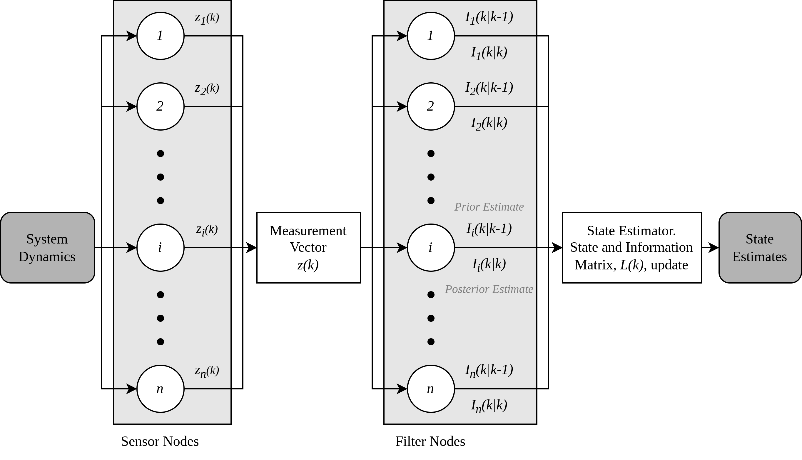
We consider the state estimation problem for an LTV system being observed with a sensor network with sensors to measure the states of the system. Fig. 1 depicts the block diagram of the DKF. Distributed estimation is carried out at the ”filter nodes”, wherein the individual prior and posterior estimates are computed, after which they are aggregated at the ”state estimator” to produce state estimates of the LTV system. While sending information to the state estimator, each sensor is associated with a stochastic communication delay. Delays typically compromise the accuracy of state estimates, hence, the goal is to select the optimal number of sensors that produce accurate-enough estimates in the presence of delays. We consider a stochastic LTV system represented by the following discrete-time model
| (1) |
where and denote the states and the system’s exogenous disturbances, respectively. It is assumed that the additive disturbances are independent . The states are assumed to be partially observable by individual sensors, with the partial measurements given by
where is the measurement vector taken from the -th sensor node at time-step , , and is the measurement noise associated with the sensor . The aggregate measurement, i.e., including measurements from all sensors, would then be expressed as
III-B Preliminaries
We now introduce the following notations: being the posterior and prior estimates of the state, respectively. The conventional KF state update equation is given by:
where is the time-varying Observer Gain (OG). We define the posteriori estimation error as , and its associated posteriori covariance matrix by . By minimizing the trace of the covariance matrix, the recursive equations for the OG and the covariance matrix are obtained as follows
| (2) | ||||
| (3) |
where .
For the purpose of brevity, we represent the KF in a compact form [5] using the Information Filter (IF) framework, wherein we define , and as the corresponding Information Matrices (IM) for the priori and posteriori state estimates, respectively. Using the IM, the expression (3) together with the OG in (2) can be written as
| (4) |
where, . We further introduce variables as Information Vectors (IV), such that , and . We then have
| (5) |
The recursive expressions for the OG and IM, in the IF framework, can therefore be derived as
| (6) | ||||
| (7) | ||||
| (8) |
where, , . In case gets close to singularity, its inverse can be replaced by the pseudo-inverse [5].
III-C Distributed Kalman Filter
At the state estimator, the difference is computed and the IM is then updated. Similarly, the corresponding IV is updated by computing . Each filter node provides its corresponding prior and posterior IM, i.e., and , and state estimates, i.e., and . This information is forwarded to the system estimator that produces the following outputs for the overall set of state estimates:
| (9) | ||||
| (10) |
IV Structural Observability and Stability Analysis
IV-A DKF with Delays
In this section, we present the modifications required for the DKF in the presence of stochastic delays. Before proceeding, we assume that the open-loop stochastic LTV system in (1) is asymptotically stable in the mean-square sense. This requires to be finite and the state transition matrix, , .
If there exists a delay , where is some time index; is unavailable from a particular filter node , leading to
(for illustration, we assume that ):
| (11) |
We observe a recursive framework tracing backwards to the estimates at time instant .
IV-B Structural Observability of the Networked System
In a networked dynamical system with a large number of nodes, the classical tests for observability that include calculating the Grammian matrix would become easily complicated when scale grows. This motivates us to look into the concept of “structural observability” to identify the number of nodes to guarantee the system observability. Initially developed in [15] for structural controllability, the theory of duality enables us to extend this concept to structural observability. Next, we briefly outline the concept of structural observability, mainly relying on the results in [16].
Definition 1
A matrix {0,} is said to be a structural matrix if each element of is either zero or a non-zero free parameter denoted by a . A matrix is called a numerical realization of if any real number is assigned to all the free parameters of .
The structured pair of matrices () is said to be structurally observable if and only if a numerical realization is observable. Structurally observable pair of matrices is observable in a wide range of parameters except in a narrow range that renders the system unobservable. Clearly, structural observability is only a necessary condition for the system to be observable in Kalman’s sense and does not prove sufficiency. In [17] it is proven that the system cannot be structurally controllable, if in the associated state-control input graph (this graph is formed by taking the states and control inputs as the vertices, wherein a directed edge between the two states and exists if is nonzero, and a directed edge between the control input and state exists if is nonzero), one cannot reach all the states, starting from any of the control input nodes. By the theory of duality, we can extend the above result to define structural observability. The pair is said to be structurally observable if and only if, in the respective graph formed by and , every state can be reached from the outputs and no dilation exists. This result also extends to linear time varying systems, as shown in [18].
IV-C Stability of DKF
A comprehensive stability analysis of DKF for LTI systems is presented in [14]. In this section, we extend that result by conducting a rigorous analysis of the stability for LTV systems using DKF and prove that the estimation error remains bounded in the mean square sense. Before stating the main result, we state the following lemma.
Lemma 1
Assume that is invertible for all . Recalling the recursive form of the IM, one can write from (7)
The following results then hold:
-
1.
The function is monotonic and non-decreasing, i.e., given two positive semi-definite matrices and , with , we have .
-
2.
For any positive semi-definite matrix , there exists a such that , .
Proof:
We can rewrite expression (7) as,
For a non-singular , above expression can be simplified to
| (12) |
Consider two distinct matrices and where . Let and . From the above simplified form of , one can conclude
Thus, we obtain , and the first part of the Lemma then follows by letting .
For the second part, let with . By using the equality (12), we can write
For any , and we have
which implies that there exists a positive scalar at each time instant such that, we have
Combining the last two expressions, we conclude that
| (13) |
The proof of the second part then follows by setting and . ∎
Theorem 1
Assume that is invertible for all and define , i.e., . Then, for each , and , we have
In other words, the IM is upper bounded by the inverse of the error covariance of the DKF estimates.
Proof:
The proof is based on mathematical induction. Assume at a time , the following inequality holds :
Define . This implies that
From the fist part of Lemma 1, one can readily conclude
The proof can be concluded since at , the initialization , i.e., , ensures that the inequality holds for any . ∎
Theorem 1 proves that the true error covariance resulting from the DKF Algorithm is upper bounded by the inverse of the corresponding IM (which is the inverse of the predicted error covariance). To prove the boundedness of the true error covariance, it would therefore be sufficient to show that individual IMs are lower bounded by a positive definite matrix. Having this, we now state the main stability result.
Theorem 2
Assume that is invertible for all and that the structured pair of matrices (), where is the structure of the system matrix with is structurally observable. Then, there exists a time instant and a positive semi-definite matrix such that
Consequently, we obtain
| . | (14) |
Proof:
From the definition of in proof of Lemma 1, we have . Hence, we can write
Further from Theorem 1, we have
Recalling that and are positive definite and the sequence can be uniformly bounded by some constant matrix , we can use the second statement of Lemma 1 to obtain the following lower bound
By applying the above two inequalities recursively, we obtain
| (15) |
Define
| (16) |
and the proof is then complete. ∎
Although the authors prove stability for a consensus based DKF algorithm in [14], the stability result holds regardless of the number of consensus steps. Clearly, from Theorems 1 and 2, one can see that the estimation error is asymptotically bounded in mean square and the DKF algorithm generates estimates with bounded mean square errors for LTV systems. Theorems 1 and 2, in their present form can only be applied for systems in which is invertible for all . Extension to the cases in which is not invertible should be investigated further.
V Sensor Selection Algorithms
V-A Greedy Subset Selection
Typically a higher number of sensor nodes results in more accurate state estimates in an ideal scenario, however, it is not always true in the presence of delays. Simulations show that (Fig. 2) in the presence of delays, the accuracy of estimates may decrease when the number of sensor nodes increases. To mitigate the effects of delay, we propose to select a subset of sensor nodes such that the compromising effect of delays is reduced by lowering the number of sensors used for estimation, while the selected sensors render a satisfactory estimation accuracy. We measure the influence of delays on the state estimates by determining the relative Maximum Deviations (MD), defined as follows:
| (17) |
We measure the influence of the measurement noise using the Mean Squared Error (MSE) between the ideal and observed estimates, and , respectively. We compute the MSE from the time where the state variables settle to of their final values. Intuitively, the influence of measurement noise can be best noticed (independent of the influence of delays) when the system settles down to its equilibrium point.
In Algorithm 1, we perform a greedy search for the best subset of nodes such that the influence of delays and measurement noise is reduced while maintaining a desired state estimate accuracy level. In each iteration, the subset selection algorithm includes all those sensor nodes with possessing delays and measurement noise variances beneath their corresponding thresholds. The search iterations start from the highest possible values for and . In each iteration, all the possible sensor nodes with lower measurement noise variances and delays are selected, based on those the DKF is implemented. The values of and in Algorithm 1 correspond to the largest measurement noise covariance and delay, respectively.
V-B Subset Selection based on Stability Criterion
We now propose a novel subset selection method to choose a subset of sensor nodes from the available nodes to ensure the estimation error covariance matrix remains bounded asymptotically, i.e., when . The advantage of this subset selection method is that, unlike the greedy algorithm, there is no need to be aware of the true state values, while the selected subset of nodes ensures the stability of the DKF in the presence of delays and noises in the collected measurements. The pseudo-code for subset selection based on stability is shown in Algorithm 2.
In Algorithm 2, is the total number of sensor nodes, is the total number of time samples, is the time instance from which the stability bound in Theorem 2 is satisfied, is a vector that contains the delays associated with the nodes, and is the sampling time of the filter. The essence of the algorithm is to calculate the value of the bounding matrix and pick nodes such that the delayed IM associated with that node, i.e., , is larger than the bound described in (16), . The algorithm includes only these nodes in the final calculation of estimates by the estimator.
Algorithm 2 always returns a set of nodes that satisfies the stability criterion in (16), and thus the order of the evaluation of the nodes by the algorithm does not affect its output. The algorithm fails to return a non-empty set of nodes only when none of the nodes satisfies the stability criterion for the specified time horizon. This occurs when the delays are larger than the estimation horizon .
Remark 1
The computational complexity of calculating in Algorithm 2 is for each , where is the dimension of the system as defined earlier.
VI Results and Discussions
Consider the problem of DKF for the following LTV stochastic system modelled in discrete time as
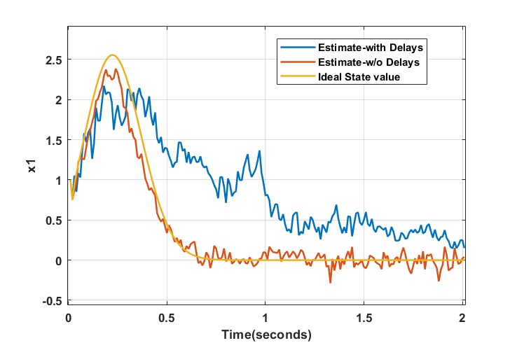
with being either or , , and the sampling time of the sensors is . We assume that there exists a transmission delay within fixed bounds from each filter node to the estimator. In this study, we consider a relatively large set of sensors by setting sensor nodes. The initial condition of the system is set to , and the system disturbance process follows . The measurement noise for the sensor nodes is Gaussian distributed with zero mean and variances belonging to the range . Communication delays are assumed to be known, belonging to the range (in seconds). {comment} The number of sensor nodes significantly affects the accuracy of the state estimates with respect to their true values. Typically in an ideal delay-free case, higher number of sensor nodes results in more precise state estimates. The influence of delays on the state estimates tends to be more pronounced by considering more nodes, which may cause undesired deviations in the transient behaviour. An illustration is shown in Fig. 2. Moreover, one can observe deviations of the estimated states from their ideal counterparts in the steady-state region. This is due to higher measurement noise variances from several sensor nodes.
The LTV system in this example, has only one time-varying element in . Thus the structural matrices for each time step in finite time can be written as
Structural observability in [16], therefore, trivially holds for the described LTV system, since the states can be reached from one another and only if while at least one of the states is being measured given being either or . Thus, the considered system is structurally observable over .
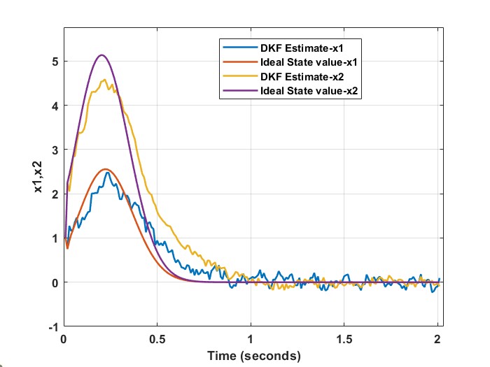
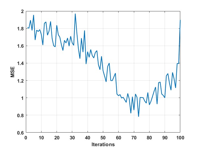
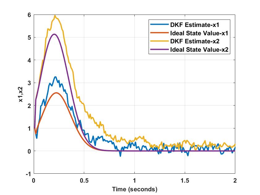
Applying Algorithm 1, as expected, by reducing the threshold values for measurement noise and delay, we observe a decreasing trend in MSE, as can be seen in Fig. 3a. However, further reduction (after the iteration) of the thresholds results in higher MSE. This is because by lowering the thresholds too low, the number of sensors satisfying the threshold conditions becomes less as well resulting in less accurate estimates. According to Fig. 3, there exists an optimal threshold where there is a trade-off between the number of selected sensors and delays along with noise levels. This observation indeed confirms the results in [19] wherein the threshold-based policies where shown to produce optimal performance when thresholds are selected properly.
{comment}
On the application of Algorithm 2, as expected, the MSE decreases on reducing the allowable set of and the delays by applying the threshold criteria. A clear decreasing trend is observable from Fig. 3a. However, on further reduction of the threshold, one can observe that the tends to increase as the number of nodes are further reduced. This is because the estimates tend to be less accurate while considering fewer nodes, irrespective of the values it may possess.
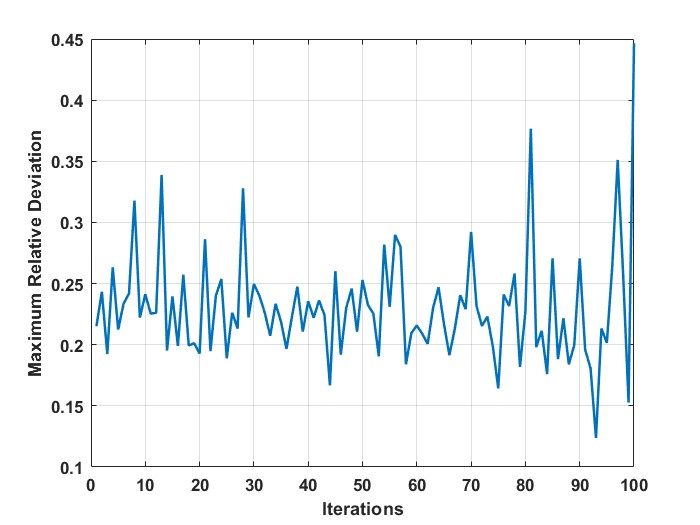
While it appears that the magnitude of the local minima for MD decreases with reducing the threshold (Fig. 3b), unlike the case of MSE, one cannot observe a unique decreasing trend for MD. One similarity with respect to the MSE in Fig. 3a is that we observe a peak in MD at the end of all iterations owing to too few nodes for estimation.
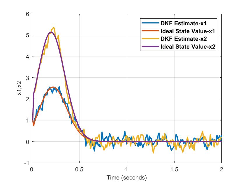
Implementing Algorithm 2 to select a subset of nodes that guarantee stability bounds, results in an estimate comparable to that of Algorithm 1. When applying Algorithm 2 and to ensure desired stability margin, should satisfy (13) when calculating . Furthermore, a reasonably small value of has to be chosen to ensure that the provided stability specifications are achievable. The estimates obtained from Algorithm 2 are illustrated in Fig. 5.
Further, Algorithm 2 is also tested to select a subset of sensor nodes with stochastic delays. Each sensor node was subject to a constant and additive stochastic delay randomly selected from . Over a Monte Carlo study of runs, it is observed that the estimates calculated from the subset of nodes with stochastic delays were comparable to the estimates computed from the subset of nodes with constant delays. A slight decrease in the MSE compared to the constant delay case is observed, which can be attributed to the lower number of selected sensor nodes. The average MSE over the trials is around 1.96 with a variance of 0.03. Moreover, the MD shows a slight increase compared to the constant delay case, with an average of 0.29 and a variance of 0.02. The number of nodes selected varied across the different runs, with an average of 22 nodes over the runs and a high variance of 14. This is expected since the number of nodes that provide a stable estimate depends on delays. Fig. 6 illustrates the simulation results of the estimates on the trials with the lowest MD.
The performances using Algorithms 1 and 2 are similar in terms of estimating the state variables, as seen from Figs. 4 and 5.
VII Conclusions
We propose a subset selection algorithm to choose a set of sensor nodes that are deemed suitable for distributed Kalman Filter state estimation in the presence of stochastic communication delays for LTV Systems. The algorithm is based on minimizing the number of sensor nodes in the subset while ensuring the stability of the state estimates. We then compare our algorithm with a greedy subset selection method that acts as a benchmark. Simulation results show comparable performance between our proposed approach and the greedy algorithm. Directions for future research include investigating stability-based node selection algorithms for DKF in partially observable LTV systems and extending the stability results under network-induced reliability and resource limitation phenomena.
VIII Conclusion & Future Work
In this work, we applied the DKF algorithm on an LTV system and proposed a novel sensor selection algorithm to derive estimates that are close to true value in the presence of bounded deterministic delays. We then derived a stability criterion for the estimates. An algorithm for selecting a subset of nodes that do not require knowledge of true estimates of the states is proposed. It produced estimates comparable to that of the lowest possible MSE given by a greedy algorithm, which serves as a benchmark. The subset selection mitigates the effect of delays caused by selecting all the nodes.
One possible direction of future research would be incorporating random delays and different mathematical models of measurement noise in the algorithms for subset selection.
References
- [1] R. Olfati-Saber. Distributed kalman filter with embedded consensus filters. In 44th IEEE Conference on Decision and Control, pages 8179–8184, 2005.
- [2] A. Speranzon, C. Fischione, K. H. Johansson, and A. Sangiovanni-Vincentelli. A distributed minimum variance estimator for sensor networks. IEEE Journal on Selected Areas in Communications, 26(4):609–621, 2008.
- [3] H. Yang, H. Li, Y. Xia, and L. Li. Distributed Kalman filtering over sensor networks with transmission delays. IEEE Trans. on Cybernetics, 51(11):5511–5521, 2021.
- [4] S. P. Talebi and S. Werner. Distributed Kalman filtering and control through embedded average consensus information fusion. IEEE Trans. on Automatic Control, 64(10):4396–4403, 2019.
- [5] M. Mesbahi and M. Egerstedt. Chapter 8: Distributed Estimation; Graph Theoretic Methods in Multiagent Networks. Princeton University Press, 2010.
- [6] H. Jin and S. Sun. Distributed Kalman filtering for sensor networks with random sensor activation, delays, and packet dropouts. Intl. Journal of Systems Science, 53(3):575–592, 2022.
- [7] G. Battistelli, L.Chisci, and D. Selvi. A distributed Kalman filter with event-triggered communication and guaranteed stability. Automatica, 93:75–82, 2018.
- [8] J. Liang, Z. Wang, B. Shen, and X. Liu. Distributed state estimation in sensor networks with randomly occurring nonlinearities subject to time delays. ACM Trans. on Sensor Networks, 9(1), 2012.
- [9] M. H. Mamduhi, A. Molin, and S. Hirche. Event-based scheduling of multi-loop stochastic systems over shared communication channels. In 21st Intl. Symposium on Mathematical Theory of Networks and Systems, 2014.
- [10] D. K. Tasoulis, N. M. Adams, and D. J. Hand. Simulation and analysis of delay handling mechanisms in sensor networks. In 10th Intl. Conf. on Computer Modeling and Simulation, pages 661–666, 2008.
- [11] M. H. Mamduhi, M. Kneissl, and S. Hirche. Decentralized event-triggered medium access control for networked control systems. In 55th IEEE Conf. on Decision and Control, pages 513–519, 2016.
- [12] H. Jin and S. Sun. Distributed filtering for sensor networks with fading measurements and compensations for transmission delays and losses. Signal Processing, 190:108306, 2022.
- [13] D. Paola, A. Petitti, and A. Rizzo. Distributed Kalman filtering via node selection in heterogeneous sensor networks. Intl. Journal of Systems Science, 46(14):2572–2583, 2015.
- [14] G. Battistelli and L. Chisci. Kullback–Leibler average, consensus on probability densities, and distributed state estimation with guaranteed stability. Automatica, 50(3):707–718, 2014.
- [15] C. Lin. Structural controllability. IEEE Trans. on Automatic Control, 19(3):201–208, 1974.
- [16] A. N. Montanari and L. A. Aguirre. Observability of network systems: A critical review of recent results. Journal of Control, Automation, and Electrical Systems, 31:1348–1374, 2020.
- [17] Y. Liu, J. Slotine, and A. Barabasi. Controllability of complex networks. Nature, 473:167–73, 2011.
- [18] G. Reissig, C. Hartung, and F. Svaricek. Strong structural controllability and observability of linear time-varying systems. IEEE Trans. on Automatic Control, 59:3087–3092, 2014.
- [19] M. H. Mamduhi, A. Molin, D. Tolic, and S. Hirche. Error-dependent data scheduling in resource-aware multi-loop networked control systems. Automatica, 81:209 – 216, 2017.