Distribution function of nuclei from scattering in the presence of a strong primordial magnetic field
Abstract
The amplitude of the primordial magnetic field (PMF) is constrained from observational limits on primordial nuclear abundances. Within this constraint, it is possible that nuclear motion is regulated by Coulomb scattering with electrons and positrons (’s), while ’s are affected by a PMF rather than collisions. For example, at a temperature of K, thermal nuclei typically experience scatterings per second that are dominated by very small angle scattering leading to minuscule changes in the nuclear kinetic energy of order (1) eV. In this paper the upper limit on the effects of a possible discretization of the momenta by the PMF on the nuclear momentum distribution is estimated under the extreme assumptions that the momentum of the is relaxed before and after Coulomb scattering to Landau levels, and that during Coulomb scattering the PMF is neglected. This assumption explicitly breaks the time reversal invariance of Coulomb scattering, and the Maxwell-Boltzmann distribution is not a trivial steady state solution of the Boltzmann equation under these assumptions. We numerically evaluate the collision terms in the Boltzmann equation, and show that the introduction of a special direction in the distribution by the PMF generates no directional dependence of the collisional destruction term of nuclei. Large anisotropies in the nuclear distribution function are then constrained from big bang nucleosynthesis. Ultimately, we conclude that a PMF does not significantly affect the isotropy or BBN.
I Introduction
In the early universe, nuclei are strongly coupled with electrons and positrons () via Coulomb scattering [1, 2]. A standard assumption during big bang nucleosynthesis (BBN) is that the nuclear energy distribution obeys Maxwell-Boltzmann (MB) statistics as a nonrelativistic approximation to the Fermi-Dirac (FD) and Bose-Einstein (BE) distribution functions [3, 4].
Simulations of nuclear motion in a relativistic plasma during the BBN epoch have been recently performed with Coulomb scatterings taken into account. It was shown that the rapid thermalization of nuclei leads to an MB distribution [2, 5]. A perturbative analysis of the relativistic Boltzmann equation shows that any fractional deviation of the thermal nuclear distribution from the MB distribution is of the order at a temperature of GK, limited by the factor of , where is the cosmic expansion rate and is the scattering rate of nuclei [6].
If there is a nonthermal particle source such as decaying exotic particles and evaporating black holes in the early universe, high energy tails in the spectra of photons and nuclei can be deformed and the BBN yields could be affected [7, 8, 9, 5]. Also, the effect of replacing an MB distribution for nuclei with Tsallis distributions [10] has been studied. It was shown that this can change the nuclear reaction rates and primordial abundances [11, 12]. Note, however, that if the nuclear distribution functions differ from MB statistics, then the relative velocity distribution depends upon the masses of reacting nuclei in contrast to the case of MB in which it only depends upon the reduced mass [13]. In addition, if the MB statistics is modified to Tsallis statistics, the phase space is changed from the simple product of the distribution functions of reacting particles as prescribed in the standard reaction theory [14].
A possible source of deviation of particle distributions from MB is the existence of a primordial magnetic field (PMF). A strong magnetic field changes weak [15, 16, 17] and nuclear [18] reaction rates, as well as thermodynamic properties of the s [19, 18] through Landau discretization of the particle momenta. In addition, the PMF energy enhances the cosmic expansion rate [20], and mainly through this effect the PMF is constrained to be G at present or G at [18, 21]. The BBN constrains PMFs generated earlier in the big bang, i.e., the electroweak phase transition [22], neutrino decoupling [23], and so on. These small-scale PMFs, however, undergo dissipation during the later cosmic evolution [24, 25, 26, 22]. This PMF evolution depends upon the helicity and homogeneity of the magnetic fields [24, 27], and its behavior in the late non-linear structure formation phase has been investigated in a number of recent three-dimensional simulations [28, 29, 30, 31]. Ultimately, what we can observe with current measurements are signatures of large-scale PMFs which could have been generated in the inflationary epoch before the big bang [32]. Constraints on the PMF [26] have been deduced from various astronomical observations such as the cosmic microwave background (CMB) temperature and polarization from gravitational [33, 34, 35, 36, 37, 38, 39] and heating effects [40], the redshifted 21-cm signal from heating effects [41, 42, 31, 43], ultra-faint dwarf galaxies from gravitational effects [44], and gravitational waves (at very small scales) [45].
It has been pointed out that an inhomogeneous PMF with a comoving amplitude of nG and a coherence length of kpc can induce chemical separations of Li+ ions from gravitationally collapsing cosmic structures [46, 47]. As a result, this sub-nG magnetic field could explain the long-standing discrepancy between the Li abundances in metal-poor stars [48, 49] and the standard BBN prediction (see Ref. [50] for the latest result based upon recent experiments on the 7Be(, )7Li reaction). Interestingly a PMF with nG over similar scales also induces baryon inhomogeneities before the epoch of cosmological recombination [51], and its effect on the CMB could also help explain the difference between Hubble parameters deduced from observations of Type Ia supernovae and the CMB [52].
The magnetic field amplitude is also constrained from the CMB power spectra and baryon acoustic oscillation data [53]. The constraint on the number of effective relativistic degrees of freedom is . This corresponds to G2 in terms of energy density, based upon the relation:
| (1) | |||||
where is the contribution from three generations of relic neutrinos and antineutrinos, and K is the present CMB temperature. The upper limit on the comoving field strength is then G. However, we caution the reader regarding three points here: (1) since most of the small-scale fields would dissipate during a long cosmic time from the BBN epoch to the time of CMB last scattering, this limit can not be compared simply with the BBN constraint. (2) The PMF affects BBN not only via the cosmic expansion rate but also changes in distribution function. Therefore, the correspondence of Eq. (1) is only an approximation even in the BBN epoch. Hence, a consistent calculation including various aspects of PMF effects [18] is necessary. (3) A rigorous calculation of the CMB including PMF effects is also required as suggested in Ref. [51].
In this letter, we show details of the collision term in the Boltzmann equation for nuclei during BBN and calculate the possible effects of a PMF on the nuclear distribution and resultant light-element abundances produced during BBN. First, it is shown that, under existing constraints on the possible amplitudes for the PMF, nuclei are predominantly affected by Coulomb scattering with s, the momenta of which are regulated by the PMF if the field strength is as high as G. Second, from a numerical integration of the collision term from Coulomb scattering, it is seen that nuclei experience very frequent scatterings most of which result in energy shifts by only . Third, the effects on the nuclear distribution function from the introduction of a discretization of momenta is analyzed. It is confirmed that the Coulomb scattering does not lead to a significant change in the nuclear isotropy and energy distributions. Finally, using a toy model, we illustrate the possible effects of a hypothetical anisotropy in the nuclear distribution function on the light elements produced during BBN.
We note that the evaluation of the collision term in the Boltzmann equation, performed here, does not depend on whether the magnetic field is homogeneous or not, on all but the smallest scales. As noted below electrons and positrons significantly change their directions on very short time scales. This means that the mean free path is very short cm. The corresponding comoving scale is only cm. At each position of a nucleus, only the magnetic field amplitude over this small scale matters. If there is an inhomogeneity in the magnetic field over this or smaller scales, the formulation here may need modification. However, the current formulation is applicable for inhomogeneity over larger scales. The purpose of the current letter is the first evaluation of detailed statistical properties of the effect of Coulomb scattering on the nuclear distribution function. We then show that for a typical upper limit on the magnetic field amplitude during BBN, the effects of magnetic fields via changes in the electron and positron distribution functions are small enough. This means that even in a universe with a spatially inhomogeneous field strength, any deviation in the nuclear distribution from a Maxwell-Boltzmann form at any location can be safely neglected.
II Timescales
First, we show that during the BBN epoch at , the motions of s are controlled by the magnetic field if the field is strong, i.e., G, while the motion of nuclei is governed by Coulomb collisions with s.
:
The gyrofrequency is a typical rate for the magnetic field effect on charged particles [54]. For it is given by
| (2) | |||||
where is the energy of the . Momentum exchange is dominated by Coulomb scatterings with abundant s during BBN. The momentum transfer cross section is estimated as follows. As a rough approximation we consider scatterings off of target particles at rest in the frame of the cosmic fluid under the nonrelativistic approximation. The maximum impact parameter is set to the Debye length given by
| (3) |
with
| (4) | |||||
| (5) |
where is the total number density of , and are the electronic charge and mass, respectively, and is the fine structure constant.
We use the relation between the scattering angle and the impact parameter,
| (6) |
where and are charge numbers of reacting particles 1 and 2, respectively, is the reduced mass, is the velocity, and is the minimum scattering angle. Then, the maximum of at is given by
| (7) | |||||
where a small angle approximation was adopted. With this maximum cosine , the momentum transfer cross section is given by
| (8) | |||||
where and are the initial momentum and the momentum transfer of , respectively, and the differential Mott cross section is given by
| (9) |
The momentum transfer rate is then given by
| (10) | |||||
The ratio of this scattering rate to the gyrofrequency is given by
| (11) | |||||
For a large enough field strength of G and , the Coulomb scattering rate is significantly smaller than the gyrofrequency. Therefore, the perturbation due to Coulomb scattering from the discretized momentum distribution would be small.
Nuclei:
Scatterings are dominated by the Coulomb scattering with . The maximum at is derived from Eq. (6) to be
| (12) |
where is the atomic number of the nucleus. The momentum transfer cross section is then given by
| (13) | |||||
where is the nuclear momentum. Accordingly, the momentum transfer rate is given by
| (14) | |||||
where is the nuclear mass number.
The ratio of this scattering rate to the gyrofrequency [Eq. (2)] is given by
| (16) | |||||
| (17) |
For a large enough field strength, G, the Coulomb scattering rate is large enough when , but diminishes relative to the gyrofrequency at lower temperatures. Since this ratio is larger than that of at , we can expect situations in which the distribution of is predominantly governed by the magnetic field while those of nuclei are determined by Coulomb collisions with in the BBN epoch.
III Model
Under the assumption of a homogeneous distribution of nonrelativistic nuclei during BBN, the invariant Boltzmann equation for nuclei in the plasma has the form of
| (18) | |||||
where is the sum of the statistical degrees of freedom of and , is the nuclear mass, is the electron energy, and are the distribution functions of nuclear momenta in the initial and final states, and , respectively, and and are the distribution functions of momenta in the initial and final states, and , respectively. The relative velocity is equal to the electron velocity in the nuclear rest frame. The quantity is the differential Mott cross section with the solid angle in the nuclear rest frame, and the is the electron energy in the nuclear rest frame.
We take the -axis as the field direction in a small local domain. The second term on the left hand side is zero if the gradient of the distribution function is proportional to the momentum along a plane perpendicular to the -axis, i.e., for and . We assume that the second term is zero hereafter. On the right hand side, the first and second terms correspond to the production and destruction, respectively, from Coulomb scattering.
When and obey an FD distribution, the quantity in the square brackets becomes zero for FD or BE distributions for nucleus . Therefore, an FD or BE distribution is a trivial steady-state solution of the Boltzmann equation, and at BBN temperatures, both of them are well approximated by an MB distribution, i.e.,
| (19) |
where is the number density of the nuclide and .
III.1 case:
When there is no magnetic field, s are assumed to have an FD distribution. Then, the production and destruction terms exactly cancel with each other. The destruction term is described by
| (20) | |||||
where is the maximum value as a function of and the angle between and , i.e., , for a fixed . The parameter , and is the azimuthal angle at the scattering. The term is from the Pauli blocking of with the momentum vector of in the final state. The quantity is the electron momentum in the nuclear rest frame, which appears in the differential Mott cross section. Note that when , , and are given, and are determined.
In the BBN epoch, the plasma has an FD distribution when there is no magnetic field, i.e., with the total energy. Unless , the electron chemical potential is negligible, and we use the same function for s.
The upper limit on the integral, i.e., appears because of the minimum scattering angle . The minimum angle is set so that the Mott scattering is ineffective if the impact parameter is larger than the Debye screening length. The effective minimum scattering angle is then given by
| (21) |
where is the plasma frequency of the background plasma.
III.2 case:
We estimate the maximum possible effect of the -field on nuclear distribution functions assuming that s in their initial states only have a discretized momentum distribution. An upper limit on the magnetic field strength is adopted from BBN studies with a PMF [18].
We assume some mechanism which only modifies the initial state momentum distribution of s, such as a PMF. An extreme case is considered here that the initial state energy spectrum is completely discretized into Landau levels. The Pauli blocking for is negligible since the initial momentum of the is discretized and the final momentum is continuous in the present application. Since most scatterings result in small (see below), transitions to different states are less important. Therefore, the Pauli blocking effect is neglected in this case.
For the case of a finite -field, the destruction term in the Boltzmann equation is described by
| (22) | |||||
| (23) |
where with and are the momentum and energy of the Landau level, is the Kronecker delta, and is the total cross section for Coulomb scattering.
In the coordinates of and , it follows that
| (24) |
IV Results
Fig. 1 shows the differential rate of change of the distribution function with respect to the final state momentum , i.e., , as a function of the change of the proton energy for scattering in the case of . The central region of small has maximum rates since the small energy changes that result from small angle scatterings have a huge cross section as long as the angle is above the lower limit. When the amplitude is larger, large angle scatterings are required. Since they occur with smaller differential cross sections, the rates are also smaller.
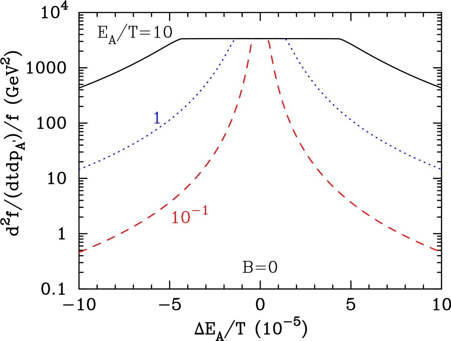
It is observed that the differential collision term has a plateau at GeV2 in the region of . The typical width of the distribution is rather consistent with the following analytical estimate. The largest contribution to the collision integral comes from the parameter region with the smallest possible scattering angle for the thermal energy of the . The minimum scattering angle for the thermal energy is given [Eq. (21)] by
| (25) |
For as in the case of thermal nuclei during the BBN epoch, we adopt an approximation that the Lorentz gamma for the nuclear velocity is , , and the angle of measured from the direction of , . Then it follows that . For this value, the change in the nuclear energy for has a typical value of
| (26) |
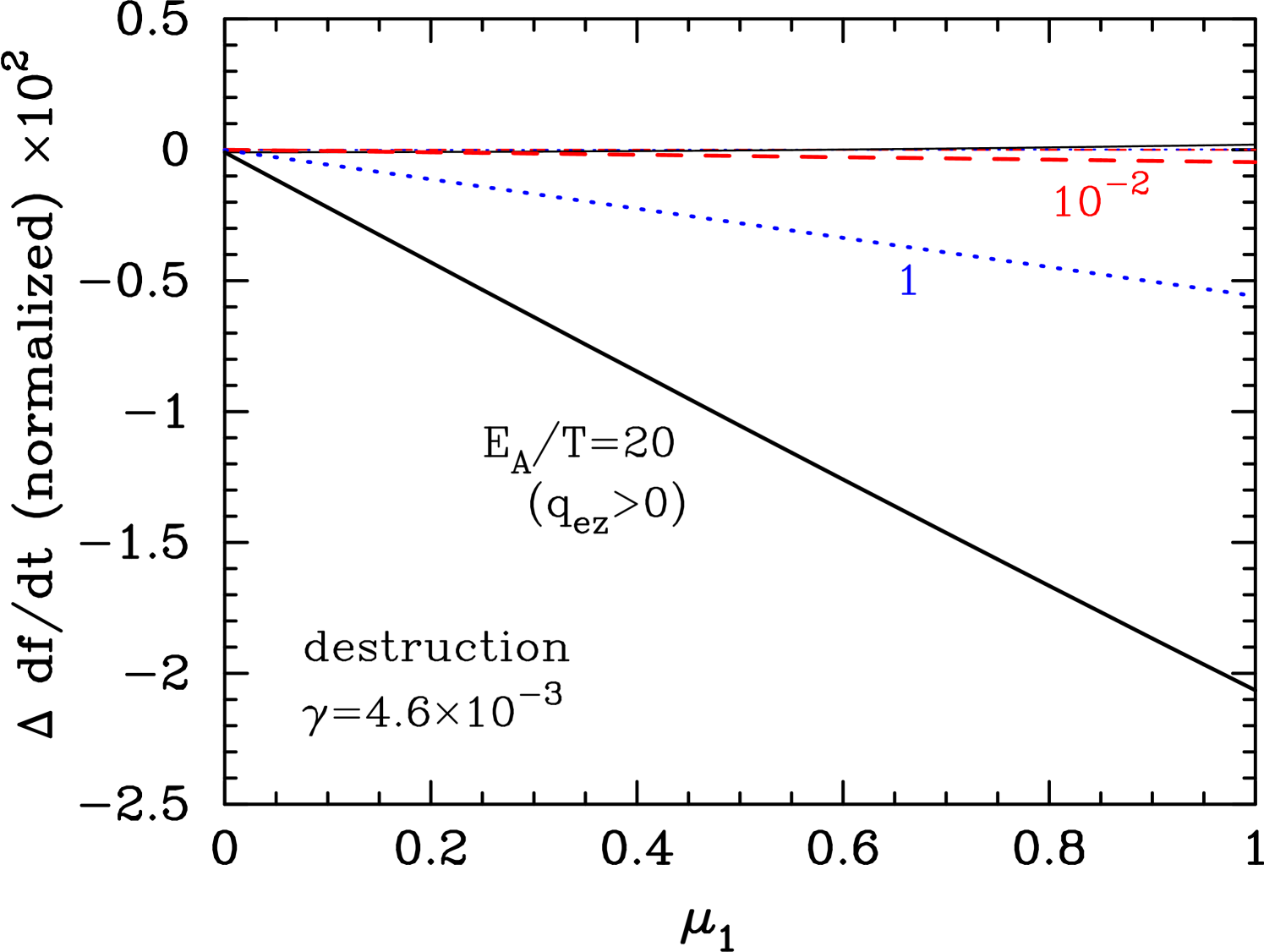
The upper panel in Fig. 2 shows the change in the destruction term of the Boltzmann equation for protons as a function of , i.e., , at K for G. The thin three lines near zero are differences in the total destruction rates. It is confirmed that the proton distribution function is independent of the direction even if the isotropy of the momentum is broken in a magnetic field. Also plotted are thick lines for the partial destruction rate by particles moving toward the hemisphere of . At high energies relevant to nuclear reactions, a significant dependence on is seen (thick solid line for ). The partial destruction rate is smaller at larger since the electron momentum in the nuclear rest frame is smaller than that in the fluid rest frame. However, after integration over the full phase space of , the dependence of the destruction rate on diminishes (thin horizontal lines).
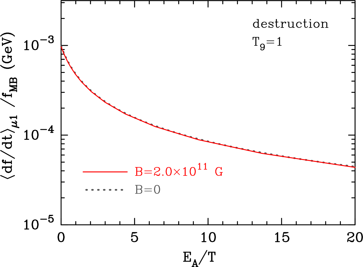
The lower panel in Fig. 2 shows the destruction term averaged over the proton direction, i.e., , as a function of the proton energy. Solid and dotted lines correspond to the results for G and 0, respectively. There is no significant difference, and it is also confirmed that the magnetic field does not affect the proton energy distribution. Note that, although the total number density is different from that of a MB distribution in a magnetic field [19], the difference is small for the upper bound on the field strength adopted here.
V Constraint on anisotropy
We derive a constraint on anisotropy in the nuclear momentum distribution during BBN. In this case, modifications to the MB distribution can be formulated as a change in the effective relative velocity distribution. Similarly to a deviation of the energy spectrum [11, 12], an introduction of anisotropy affects nucleosynthesis. As an example, we assume that the densities of particles moving in some special direction are enhanced, as described by (for ) and 0 (otherwise). Similar to Ref. [13], the relative velocity distribution function can then be written as
| (27) | |||||
where and are the normalization constants, and are masses of reacting particles 1 and 2, , is the center of mass (CM) velocity, while and are, respectively, the cosine of the polar angle and azimuthal angle at the scattering.
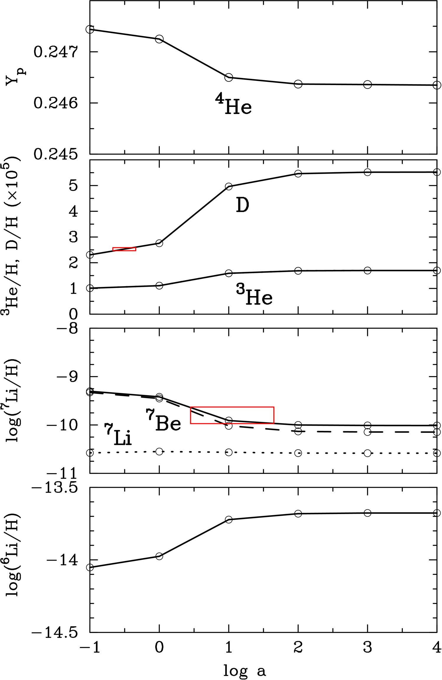
Figure 3 shows light element abundances as a function of the anisotropy parameter in the BBN model including the anisotropy in all nuclear distribution functions. The introduction of this type of anisotropy causes larger energies of the CM, i.e., , and smaller relative energies in the CM system, i.e., . As a result, a larger leads to a softer distribution of with a smaller average. Then, nuclear reaction rates are hindered and light element abundances are changed in a similar manner as in the case where the isotropic distribution function deviates from a MB distribution to the softer side. The dependencies of abundances on anisotropy is very similar to those of a spectral distortion [12, 13].
VI Summary
The effect of Landau discretization of the momenta on the collision term of protons during BBN was studied. At K, nuclei experience scatterings per second from , and most of the scatterings lead to small, (1) eV, changes of the nuclear kinetic energy. When the magnetic field amplitude is set to the largest value allowed by observations, the distribution experiencing the magnetic field does not lead to any significant directional dependence in the collisional destruction term of nuclei. A constraint on the amplitude of anisotropies in the nuclear distribution function during BBN was also derived.
Acknowledgements.
This work is supported by NSFC Research Fund for International Young Scientists (Grant No. 11850410441). Work at the University of Notre Dame supported by DOE nuclear theory grant DE-FG02-95-ER40934.References
- Voronchev et al. [2008] V. T. Voronchev, Y. Nakao, and M. Nakamura, Non-thermal processes in standard big bang nucleosynthesis. I: In-flight nuclear reactions induced by energetic protons, JCAP 05, 010.
- Sasankan et al. [2020] N. Sasankan, A. Kedia, M. Kusakabe, and G. J. Mathews, Analysis of the Multi-component Relativistic Boltzmann Equation for Electron Scattering in Big Bang Nucleosynthesis, Phys. Rev. D 101, 123532 (2020), arXiv:1911.07334 [nucl-th] .
- Hayashi and Nishida [1956] C. Hayashi and M. Nishida, Formation of Light Nuclei in the Expanding Universe, Progress of Theoretical Physics 16, 613 (1956).
- Wagoner et al. [1967] R. V. Wagoner, W. A. Fowler, and F. Hoyle, On the Synthesis of elements at very high temperatures, Astrophys. J. 148, 3 (1967).
- Kedia et al. [2021] A. Kedia, N. Sasankan, G. J. Mathews, and M. Kusakabe, Simulations of multicomponent relativistic thermalization, Phys. Rev. E 103, 032101 (2021), arXiv:2004.13186 [cond-mat.stat-mech] .
- McDermott and Turner [2018] S. D. McDermott and M. S. Turner, Nuclear Kinetic Equilibrium During Big Bang Nucleosynthesis, (2018), arXiv:1811.04932 [hep-ph] .
- Lindley [1979] D. Lindley, Radiative decay of massive neutrinos and cosmic element abundances., Mon. Not. R. Astron. Soc. 188, 15P (1979).
- Reno and Seckel [1988] M. H. Reno and D. Seckel, Primordial nucleosynthesis: The effects of injecting hadrons, Phys. Rev. D 37, 3441 (1988).
- Dimopoulos et al. [1988] S. Dimopoulos, R. Esmailzadeh, L. J. Hall, and G. D. Starkman, Is the Universe Closed by Baryons? Nucleosynthesis with a Late-decaying Massive Particle, Astrophys. J. 330, 545 (1988).
- Tsallis [1988] C. Tsallis, Possible Generalization of Boltzmann-Gibbs Statistics, J. Statist. Phys. 52, 479 (1988).
- Bertulani et al. [2013] C. Bertulani, J. Fuqua, and M. Hussein, Big Bang nucleosynthesis with a non-Maxwellian distribution, Astrophys. J. 767, 67 (2013), arXiv:1205.4000 [nucl-th] .
- Hou et al. [2017] S. Hou, J. He, A. Parikh, D. Kahl, C. Bertulani, T. Kajino, G. Mathews, and G. Zhao, Non-extensive Statistics to the Cosmological Lithium Problem, Astrophys. J. 834, 165 (2017), arXiv:1701.04149 [astro-ph.CO] .
- Kusakabe et al. [2019] M. Kusakabe, T. Kajino, G. J. Mathews, and Y. Luo, On the relative velocity distribution for general statistics and an application to big-bang nucleosynthesis under Tsallis statistics, Phys. Rev. D 99, 043505 (2019), arXiv:1806.01454 [astro-ph.CO] .
- Rueter et al. [2019] T. D. Rueter, T. G. Rizzo, and J. L. Hewett, Dark Matter Freeze Out with Tsallis Statistics in the Early Universe, (2019), arXiv:1911.11254 [hep-ph] .
- O’Connell and Matese [1969] R. F. O’Connell and J. J. Matese, Effect of a Constant Magnetic Field on the Neutron Beta Decay Rate and its Astrophysical Implications, Nature (London) 222, 649 (1969).
- Cheng et al. [1996] B.-l. Cheng, A. V. Olinto, D. N. Schramm, and J. W. Truran, Constraints on the strength of primordial magnetic fields from big bang nucleosynthesis revisited, Phys. Rev. D54, 4714 (1996).
- Luo et al. [2020] Y. Luo, M. A. Famiano, T. Kajino, M. Kusakabe, and A. B. Balantekin, Screening corrections to Electron Capture Rates and resulting constraints on Primordial Magnetic Fields, Phys. Rev. D 101, 083010 (2020), arXiv:2002.08636 [astro-ph.CO] .
- Kawasaki and Kusakabe [2012] M. Kawasaki and M. Kusakabe, Updated constraint on a primordial magnetic field during big bang nucleosynthesis and a formulation of field effects, Phys. Rev. D 86, 063003 (2012), arXiv:1204.6164 [astro-ph.CO] .
- Kernan et al. [1996] P. J. Kernan, G. D. Starkman, and T. Vachaspati, Big bang nucleosynthesis constraints on primordial magnetic fields, Phys. Rev. D 54, 7207 (1996), arXiv:astro-ph/9509126 .
- Greenstein [1969] G. Greenstein, Primordial Helium Production in “Magnetic” Cosmologies, Nature (London) 223, 938 (1969).
- Luo et al. [2019] Y. Luo, T. Kajino, M. Kusakabe, and G. J. Mathews, Big Bang Nucleosynthesis with an Inhomogeneous Primordial Magnetic Field Strength, Astrophys. J. 872, 172 (2019), arXiv:1810.08803 [astro-ph.CO] .
- Vachaspati [2021] T. Vachaspati, Progress on cosmological magnetic fields, Rept. Prog. Phys. 84, 074901 (2021), arXiv:2010.10525 [astro-ph.CO] .
- Dolgov and Grasso [2001] A. D. Dolgov and D. Grasso, Generation of cosmic magnetic fields and gravitational waves at neutrino decoupling, Phys. Rev. Lett. 88, 011301 (2001), arXiv:astro-ph/0106154 .
- Brandenburg and Matthaeus [2004] A. Brandenburg and W. H. Matthaeus, Magnetic helicity evolution in a periodic domain with imposed field, Phys. Rev. E 69, 056407 (2004), arXiv:astro-ph/0305373 .
- Banerjee and Jedamzik [2004] R. Banerjee and K. Jedamzik, The Evolution of cosmic magnetic fields: From the very early universe, to recombination, to the present, Phys. Rev. D 70, 123003 (2004), arXiv:astro-ph/0410032 .
- Widrow et al. [2012] L. M. Widrow, D. Ryu, D. R. Schleicher, K. Subramanian, C. G. Tsagas, and R. A. Treumann, The First Magnetic Fields, Space Sci. Rev. 166, 37 (2012), arXiv:1109.4052 [astro-ph.CO] .
- Brandenburg et al. [2020] A. Brandenburg, R. Durrer, Y. Huang, T. Kahniashvili, S. Mandal, and S. Mukohyama, Primordial magnetic helicity evolution with a homogeneous magnetic field from inflation, Phys. Rev. D 102, 023536 (2020), arXiv:2005.06449 [astro-ph.CO] .
- Hutschenreuter et al. [2018] S. Hutschenreuter, S. Dorn, J. Jasche, F. Vazza, D. Paoletti, G. Lavaux, and T. A. Enßlin, The primordial magnetic field in our cosmic backyard, Class. Quant. Grav. 35, 154001 (2018), arXiv:1803.02629 [astro-ph.CO] .
- Sanati et al. [2020] M. Sanati, Y. Revaz, J. Schober, K. E. Kunze, and P. Jablonka, Constraining the primordial magnetic field with dwarf galaxy simulations, Astron. Astrophys. 643, A54 (2020), arXiv:2005.05401 [astro-ph.GA] .
- Vazza et al. [2020] F. Vazza, D. Paoletti, S. Banfi, F. Finelli, C. Gheller, S. P. O’Sullivan, and M. Brüggen, Simulations and observational tests of primordial magnetic fields from Cosmic Microwave Background constraintsok, Mon. Not. Roy. Astron. Soc. 500, 5350 (2020), arXiv:2009.01539 [astro-ph.CO] .
- Katz et al. [2021] H. Katz et al., Introducing SPHINX-MHD: The Impact of Primordial Magnetic Fields on the First Galaxies, Reionization, and the Global 21cm Signal, (2021), arXiv:2101.11624 [astro-ph.CO] .
- Ratra [1992] B. Ratra, Cosmological “Seed” Magnetic Field from Inflation, Astrophys. J. Lett. 391, L1 (1992).
- Zucca et al. [2017] A. Zucca, Y. Li, and L. Pogosian, Constraints on Primordial Magnetic Fields from Planck combined with the South Pole Telescope CMB B-mode polarization measurements, Phys. Rev. D 95, 063506 (2017), arXiv:1611.00757 [astro-ph.CO] .
- Ade et al. [2017] P. A. R. Ade et al. (BICEP2, Keck Arrary), BICEP2 / Keck Array IX: New bounds on anisotropies of CMB polarization rotation and implications for axionlike particles and primordial magnetic fields, Phys. Rev. D 96, 102003 (2017), arXiv:1705.02523 [astro-ph.CO] .
- Sutton et al. [2017] D. R. Sutton, C. Feng, and C. L. Reichardt, Current and Future Constraints on Primordial Magnetic Fields, Astrophys. J. 846, 164 (2017), arXiv:1702.01871 [astro-ph.CO] .
- Pogosian and Zucca [2018] L. Pogosian and A. Zucca, Searching for Primordial Magnetic Fields with CMB B-modes, Class. Quant. Grav. 35, 124004 (2018), arXiv:1801.08936 [astro-ph.CO] .
- Yamazaki [2018] D. G. Yamazaki, Impact of a primordial magnetic field on cosmic microwave background modes with weak lensing, Phys. Rev. D 97, 103525 (2018), arXiv:1805.09903 [astro-ph.CO] .
- Paoletti et al. [2019] D. Paoletti, J. Chluba, F. Finelli, and J. A. Rubino-Martin, Improved CMB anisotropy constraints on primordial magnetic fields from the post-recombination ionization history, Mon. Not. Roy. Astron. Soc. 484, 185 (2019), arXiv:1806.06830 [astro-ph.CO] .
- Minoda et al. [2021] T. Minoda, K. Ichiki, and H. Tashiro, Small-scale CMB anisotropies induced by the primordial magnetic fields, JCAP 03, 093, arXiv:2012.12542 [astro-ph.CO] .
- Paoletti and Finelli [2019] D. Paoletti and F. Finelli, Constraints on primordial magnetic fields from magnetically-induced perturbations: current status and future perspectives with LiteBIRD and future ground based experiments, JCAP 11, 028, arXiv:1910.07456 [astro-ph.CO] .
- Minoda et al. [2019] T. Minoda, H. Tashiro, and T. Takahashi, Insight into primordial magnetic fields from 21-cm line observation with EDGES experiment, Mon. Not. Roy. Astron. Soc. 488, 2001 (2019), arXiv:1812.00730 [astro-ph.CO] .
- Natwariya [2021] P. K. Natwariya, Constraint on Primordial Magnetic Fields In the Light of ARCADE 2 and EDGES Observations, Eur. Phys. J. C 81, 394 (2021), arXiv:2007.09938 [astro-ph.CO] .
- Bera et al. [2020] A. Bera, K. K. Datta, and S. Samui, Primordial magnetic fields during the cosmic dawn in light of EDGES 21-cm signal, Mon. Not. Roy. Astron. Soc. 498, 918 (2020), arXiv:2005.14206 [astro-ph.CO] .
- Safarzadeh and Loeb [2019] M. Safarzadeh and A. Loeb, An upper limit on primordial magnetic fields from ultra-faint dwarf galaxies, Astrophys. J. Lett. 877, L27 (2019), arXiv:1901.03341 [astro-ph.CO] .
- Saga et al. [2018] S. Saga, H. Tashiro, and S. Yokoyama, Limits on primordial magnetic fields from direct detection experiments of gravitational wave background, Phys. Rev. D 98, 083518 (2018), arXiv:1807.00561 [astro-ph.CO] .
- Kusakabe and Kawasaki [2015] M. Kusakabe and M. Kawasaki, Chemical separation of primordial Li+ during structure formation caused by nanogauss magnetic field, Mon. Not. Roy. Astron. Soc. 446, 1597 (2015), arXiv:1404.3485 [astro-ph.CO] .
- Kusakabe and Kawasaki [2019] M. Kusakabe and M. Kawasaki, Initial Li Abundances in the Proto-Galaxy and Globular Clusters Based upon the Chemical Separation and Hierarchical Structure Formation, Astrophys. J. Lett. 876, L30 (2019), arXiv:1903.08035 [astro-ph.SR] .
- Spite and Spite [1982] F. Spite and M. Spite, Abundance of lithium in unevolved halo stars and old disk stars: Interpretation and consequences, Astron. Astrophys. 115, 357 (1982).
- Sbordone et al. [2010] L. Sbordone et al., The metal-poor end of the Spite plateau. 1: Stellar parameters, metallicities and lithium abundances, Astron. Astrophys. 522, A26 (2010), arXiv:1003.4510 [astro-ph.GA] .
- Hayakawa et al. [2021] S. Hayakawa et al., Constraining the Primordial Lithium Abundance: New Cross Section Measurement of the 7Be + n Reactions Updates the Total 7Be Destruction Rate, Astrophys. J. Lett. 915, L13 (2021).
- Jedamzik and Pogosian [2020] K. Jedamzik and L. Pogosian, Relieving the Hubble tension with primordial magnetic fields, Phys. Rev. Lett. 125, 181302 (2020), arXiv:2004.09487 [astro-ph.CO] .
- Reid et al. [2019] M. J. Reid, D. W. Pesce, and A. G. Riess, An Improved Distance to NGC 4258 and its Implications for the Hubble Constant, Astrophys. J. Lett. 886, L27 (2019), arXiv:1908.05625 [astro-ph.GA] .
- Aghanim et al. [2020] N. Aghanim et al. (Planck), Planck 2018 results. VI. Cosmological parameters, Astron. Astrophys. 641, A6 (2020), arXiv:1807.06209 [astro-ph.CO] .
- Jackson [1975] J. D. Jackson, Classical electrodynamics 2nd ed. (John Wiley & Sons, New York, 1975).