Distributionally Robust Model Predictive Control with Mixture of Gaussian Processes*

To accommodate the state-dependent property, we tailor the Dirichlet process to serve as an input-dependent gating network. In the standard Dirichlet process with the concentration parameter $\alpha$, the conditional probability of the indicator variable $c_{i}$ is given by

where $n_{-i,j}=\sum_{i^{\prime}\neq i}\delta(c_{i^{\prime}},j)$ represents the number of data points in expert $j$ excluding observation $i$, and $n$ is the total number of data points. To incorporate input dependence into the gating network, we redefine $n_{-i,j}$ as follows.

where $K_{\phi}$ is a kernel function parametrized by $\phi$ and $\delta$ is the Dirac delta function. Consequently, given a new data point, the conditional distribution of its indicator variable can be obtained by substituting (5) into (4).

For a local GP expert $j$, let $\mathbf{z}=\{z_{1},\ldots z_{N}\}$ represent the training inputs and $\mathbf{y}=\{y_{1},\ldots,y_{N}\}$ denote the corresponding noisy outputs, where $y_{i}=w(z_{i})+\epsilon_{i}$. The observation noise $\epsilon_{i}$ is assumed to be i.i.d, following a normal distribution with mean $0$ and variance $\Sigma_{on}=\text{diag}\{\sigma_{1}^{2},\ldots,\sigma_{n}^{2}\}$. Each output dimension is modeled independently. For dimension $j$, we define a GP prior with kernel $k(\cdot,\cdot)$ and mean function $m(\cdot)$. Conditioning on the data $\mathbf{z}$ and $\mathbf{y}^{(j)}=\{y_{1}^{(j)},\ldots,y_{N}^{(j)}\}$, the predictive posterior distribution for the output at a new data point $z^{*}$ is Gaussian with the following mean and variance.

where $K_{\sigma_{j}}=k\left({\mathbf{z},\mathbf{z}}\right)+\sigma_{j}^{2}I$.

Based on the above analysis, the predictive distribution of $w(z^{*})$ in dimension $a$ generated by MoGP can be expressed by combining the conditional distributions of the indicator variables from the gating network with the results from local GP regression, as shown in (7).

where $M$ is the number of experts, $\mathcal{D}$ represents the training dataset, and $\gamma_{a,j}$ denotes the weight of the corresponding Gaussian component obtained by Dirichlet process. This formulation effectively captures the potential multimodalities in the latent function. However, errors between the predictive distribution and the true underlying distribution still exists. To mitigate this uncertainty, we construct an ambiguity set in the following section.

To formulate the DR-CVaR constraints on system states, we construct a state-dependent ambiguity set that accounts for potential multimodalities by leveraging the MoGP model for $w(\cdot)$ in each dimension. Particularly, given a specific system state $x^{*}$ at time $t$, suppose that the predictive distribution for $w(x^{*})$ in dimension $\tau$, which consists of $M_{\tau}$ state-dependent Gaussian components, can be written as

Considering the structure of modalities and independence between each mode, we establish local ambiguity sets using the state-dependent mean and variance information from the Gaussian components in (9). The overall ambiguity set $\mathcal{W}_{\tau}(x^{*})$ is then constructed as a weighted Minkowski sum of these local ambiguity sets. Explicitly, each local state-dependent ambiguity set $\mathcal{W}_{\tau,j}$ is defined below.

where $\mathcal{M}_{+}$ represents the set of positive Borel measure on $\mathbb{R}$, and $\rho$ is a positive measure. The proposed ambiguity set $\mathcal{W}_{\tau}(x^{*})$ is defined as

This construction closely aligns with the potentially multimodal structure, allowing for a more flexible and intricate representation of state-dependent disturbances.

Define $x_{k|t}$ as the $k$ step ahead predicted system state based on the current state $x_{t}$, while $x_{0|t}=x_{t}$ is the given initial state. To ensure recursive feasibility, we adopt a hybrid constraint tightening strategy that combines distributionally robust and worst-case tightening methods.

For $x_{1|t}$, the corresponding DR-CVaR constraint can be expressed as follows [16].

Noting that $x_{1|t}=(A+BK)x_{0|t}-BKs_{0|t}+Bv_{0|t}+w(x_{0|t})$, since the state-dependent term $w(x_{0|t})$ is the only source of uncertainty, the ambiguity set $Q_{\tau}(x_{1|t})$ is essentially a shifted version of the ambiguity set for $w(x_{0|t})^{(\tau)}$, denoted as $\mathcal{W}_{\tau}(x_{0|t})$. Hence, it can be defined in the same manner as (11). Based on (11), we consequently prove that Constraint (12) can be equivalently reformulated as second-order cone constraints in the subsequent section.

Given the support set $\mathbb{W}$, we define $\mathcal{Z}$ as the minimal Robust Positively Invariant (mRPI) set for the error dynamics in (8b). The remaining system constraints are then guaranteed by the tightened state constraints $s_{k|t}\in\mathbb{X}\ominus\mathcal{Z},k\in\{2,\ldots,N-1\}$ and input constraints $v_{k|t}\in\mathbb{U}\ominus K\mathcal{Z},k\in\{0,\ldots,N-1\}$ [17]. Additionally, the constraint $x_{t}-s_{0|t}\in\mathcal{Z}$ is required to be satisfied. Finally, we impose the terminal constraint $s_{N|t}\in\mathcal{X}_{f}$, where $\mathcal{X}_{f}$ is defined in (13).

Based on the above analysis, the formulation of MoGP-DR-MPC at time $t$, denoted as $\mathscr{P}(x_{t})$, is written as

where $\mathbf{v}_{t}=[v_{0|t}\ldots v_{N-1|t}]^{\top}$ and $P,Q,R$ are positive definite weight matrices, with $P$ determined through the Riccati equation. Obviously, Problem $\mathscr{P}(x_{t})$ is nonconvex and cannot be solved directly due to the presence of constraint (14e). We then derive its equivalent tractable form in the next section.

In this section, we demonstrate how to transform the critical and intractable DR-CVaR constraint (14e) into a set of second-order cone constraints using the following theorem.

Theorem 1 provides the convex reformulation alternatives of Constraint (14e). It follows that the optimization problem $\mathscr{P}(x_{t})$ can be reformulated into the convex and tractable form below, which is denoted as $\mathscr{P}_{MoDR}(x_{t})$.

If $\mathscr{P}_{MoDR}(x_{t})$ is feasible at time $t$, let $s_{0|t}^{*}$ and $\mathbf{v}_{t}^{*}=[v_{0|t}^{*},\ldots,v_{N-1|t}^{*}]^{\top}$ represent its optimal solution. At each time instant, the MoGP-DR-MPC framework solves $\mathscr{P}_{MoDR}(x_{t})$ to obtain the optimal input sequence and only the first element $u_{t}^{*}=K(x_{t}-s_{0|t}^{*})+v_{0|t}^{*}$ is executed. This process is repeated to perform receding horizon control.

We first conduct numerical experiments on a stochastic system given in (26).

Suppose the constraint sets are $\mathbb{X}=[-7,0]\times[-3,2]$ and $\mathbb{U}=[-5,5]$, with a tolerance level of $\varepsilon=0.2$. Disturbance $w(x)$ is supported by $[-0.8,0.8]\times[-0.8,0.8]$ and is defined using standard four-modal function i.e. Franke function [21] in each dimension. The control objective is to steer the initial state $[-5,-2]$ to the origin under the disturbance $w(x)$. Define the stage cost as $x^{\top}Qx+u^{\top}Ru$, where $Q$ is identity matrix $I_{2}$ and $R=0.1$. The horizon of MPC is set as $10$ and we perform 50 closed-loop simulations with a simulation horizon of 30 to showcase the improvement in control performance.

The average closed-loop costs for MoGP-DR-MPC, GP-DR-MPC and robust tube MPC are 66.06, 79.74 and 89.22, respectively. The simulation results indicate that MoGP-DR-MPC reduces the average closed-loop cost by 17% compared with GP-DR-MPC and by 24% compared with robust tube MPC, demonstrating its notable advantage in handling multimodal state-dependent disturbances.

In the second case study, we simulate a trajectory planning and control problem for a planar quadrotor system [22]. The quadrotor starts at $(10,10)$ and is expected to land at the origin. During its flight, it must remain within the safe region $\mathcal{X}$ with probability $0.8$ under a multimodal state-dependent wind disturbance, which is common due to varying airflow patterns. The linearized dynamics of the quadrotor system are expressed as follows.

where $\Delta t=1$ is the sampling time and $m$ represents the mass of the system. The state vector $s_{t}=[p_{x},v_{x},p_{y},v_{y}]^{\top}\in\mathbb{R}^{4}$ includes the quadrotor’s positions and velocities in the $x$ and $y$ directions, while the control input $u_{t}=[u_{x},u_{y}]^{\top}\in[-7,7]^{2}\subseteq\mathbb{R}^{2}$ applies forces along these axes. The support set of the wind disturbance is represented by $\mathbb{W}=[-0.6,0.6]^{4}\subseteq\mathbb{R}^{4}$ and the safe region $\mathcal{X}$ is defined by

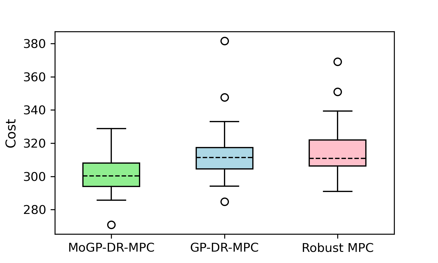
In the simulations, the MPC time horizon $N$ is set to five and we evaluate the performance of MoGP-DR-MPC against two baseline approaches. Specifically, we analyze the closed-loop costs under 50 different sequences of disturbance realizations, each with 30 simulation steps. As illustrated in Fig 1, MoGP-DR-MPC achieves an average reduction in closed-loop cost of 4% compared with GP-DR-MPC and 5% compared with robust tube MPC. This corroborates the superior ability of MoGP-DR-MPC to capture the multimodal characteristics of disturbance data, yielding less conservative control performance.

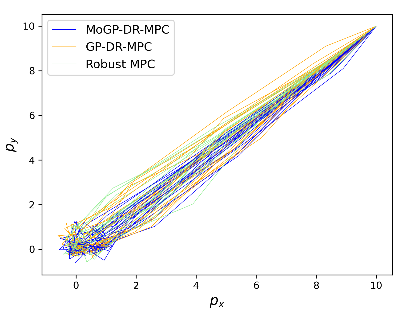
Additionally, because the optimal control problem is convex and the MoGP model is trained offline, the computation time for MoGP-DR-MPC is on par with that of conventional GP-MPC. Fig 2 shows the position trajectories of the quadrotor generated by 30 simulations.

References

- [1] F. Berkenkamp and A. P. Schoellig, “Safe and robust learning control with gaussian processes,” in 2015 European Control Conference (ECC). IEEE, 2015, pp. 2496–2501.
- [2] Y. Wang, C. Ocampo-Martinez, and V. Puig, “Robust model predictive control based on gaussian processes: Application to drinking water networks,” in 2015 European Control Conference (ECC), 2015, pp. 3292–3297.
- [3] A. Rose, M. Pfefferkorn, H. H. Nguyen, and R. Findeisen, “Learning a gaussian process approximation of a model predictive controller with guarantees,” in 2023 62nd IEEE Conference on Decision and Control (CDC). IEEE, 2023, pp. 4094–4099.
- [4] E. Bradford, L. Imsland, D. Zhang, and E. A. del Rio Chanona, “Stochastic data-driven model predictive control using gaussian processes,” Computers & Chemical Engineering, vol. 139, p. 106844, 2020.
- [5] L. Hewing, J. Kabzan, and M. N. Zeilinger, “Cautious model predictive control using gaussian process regression,” IEEE Transactions on Control Systems Technology, vol. 28, no. 6, pp. 2736–2743, 2019.
- [6] A. Capone, T. Brüdigam, and S. Hirche, “Online constraint tightening in stochastic model predictive control: A regression approach,” IEEE Transactions on Automatic Control, pp. 1–15, 2024, doi: 10.1109/TAC.2024.3433988.
- [7] B. Li, T. Guan, L. Dai, and G.-R. Duan, “Distributionally robust model predictive control with output feedback,” IEEE Transactions on Automatic Control, vol. 69, no. 5, pp. 3270–3277, 2024.
- [8] K. Kim and I. Yang, “Distributional robustness in minimax linear quadratic control with wasserstein distance,” SIAM Journal on Control and Optimization, vol. 61, no. 2, pp. 458–483, 2023.
- [9] C. Mark and S. Liu, “Recursively feasible data-driven distributionally robust model predictive control with additive disturbances,” IEEE Control Systems Letters, vol. 7, pp. 526–531, 2022.
- [10] G. Pan and T. Faulwasser, “Distributionally robust uncertainty quantification via data-driven stochastic optimal control,” IEEE Control Systems Letters, vol. 7, pp. 3036–3041, 2023.
- [11] F. Micheli, T. Summers, and J. Lygeros, “Data-driven distributionally robust mpc for systems with uncertain dynamics,” in 2022 IEEE 61st Conference on Decision and Control (CDC). IEEE, 2022, pp. 4788–4793.
- [12] A. Hakobyan and I. Yang, “Learning-based distributionally robust motion control with gaussian processes,” in 2020 IEEE/RSJ International Conference on Intelligent Robots and Systems (IROS). IEEE, 2020, pp. 7667–7674.
- [13] F. Li, H. Li, and Y. He, “Adaptive stochastic model predictive control of linear systems using gaussian process regression,” IET Control Theory & Applications, vol. 15, no. 5, pp. 683–693, 2021.
- [14] C. Ning and F. You, “Online learning based risk-averse stochastic mpc of constrained linear uncertain systems,” Automatica, vol. 125, p. 109402, 2021.
- [15] C. Rasmussen and Z. Ghahramani, “Infinite mixtures of gaussian process experts,” Advances in neural information processing systems, vol. 14, 2001.
- [16] B. P. Van Parys, D. Kuhn, P. J. Goulart, and M. Morari, “Distributionally robust control of constrained stochastic systems,” IEEE Transactions on Automatic Control, vol. 61, no. 2, pp. 430–442, 2015.
- [17] D. Q. Mayne, M. M. Seron, and S. V. Raković, “Robust model predictive control of constrained linear systems with bounded disturbances,” Automatica, vol. 41, no. 2, pp. 219–224, 2005.
- [18] G. A. Hanasusanto, D. Kuhn, S. W. Wallace, and S. Zymler, “Distributionally robust multi-item newsvendor problems with multimodal demand distributions,” Mathematical Programming, vol. 152, no. 1, pp. 1–32, 2015.
- [19] S. Boyd and L. Vandenberghe, Convex optimization. Cambridge university press, 2004.
- [20] L. Li, C. Ning, H. Qiu, W. Du, and Z. Dong, “Online data-stream-driven distributionally robust optimal energy management for hydrogen-based multimicrogrids,” IEEE Transactions on Industrial Informatics, vol. 20, no. 3, pp. 4370–4384, 2024.
- [21] R. Franke, A critical comparison of some methods for interpolation of scattered data. Naval Postgraduate School Monterey, CA, 1979.
- [22] Y. K. Nakka, R. C. Foust, E. S. Lupu, D. B. Elliott, I. S. Crowell, S.-J. Chung, and F. Y. Hadaegh, “A six degree-of-freedom spacecraft dynamics simulator for formation control research,” in 2018 AAS/AIAA Astrodynamics Specialist Conference, 2018, pp. 1–20.