11email: lfq20@mails.tsinghua.edu.cn
4Paradigm Inc., Beijing, 100084, China
11email: {huangshiyu,tuweiwei}@4paradigm.com
Diverse Policies Converge in Reward-free Markov Decision Processes
Abstract
Reinforcement learning has achieved great success in many decision-making tasks, and traditional reinforcement learning algorithms are mainly designed for obtaining a single optimal solution. However, recent works show the importance of developing diverse policies, which makes it an emerging research topic. Despite the variety of diversity reinforcement learning algorithms that have emerged, none of them theoretically answer the question of how the algorithm converges and how efficient the algorithm is. In this paper, we provide a unified diversity reinforcement learning framework and investigate the convergence of training diverse policies. Under such a framework, we also propose a provably efficient diversity reinforcement learning algorithm. Finally, we verify the effectiveness of our method through numerical experiments111Access the code on GitHub: https://github.com/OpenRL-Lab/DiversePolicies.
Keywords:
Reinforcement learning Diversity Reinforcement Learning Bandit.1 Introduction
Reinforcement learning (RL) shows huge advantages in various decision-making tasks, such as recommendation systems [20, 23], game AIs [3, 10] and robotic controls [24, 17]. While traditional RL algorithms can achieve superhuman performances on many public benchmarks, the obtained policy often falls into a fixed pattern. For example, previously trained agents may just overfit to a determined environment and could be vulnerable to environmental changes [6]. Finding diverse policies may increase the robustness of the agent [16, 12]. Moreover, a fixed-pattern agent will easily be attacked [21], because the opponent can find its weakness with a series of attempts. If the agent could play the game with different strategies each round, it will be hard for the opponent to identify the upcoming strategy and it will be unable to apply corresponding attacking tactics [13]. Recently, developing RL algorithms for diverse policies has attracted the attention of the RL community for the promising value of its application and also for the challenge of solving a more complex RL problem [7, 11, 4].
Current diversity RL algorithms vary widely due to factors like policy diversity measurement, optimization techniques, training strategies, and application scenarios. This variation makes comparison challenging. While these algorithms often incorporate deep neural networks and empirical tests for comparison, they typically lack in-depth theoretical analysis on training convergence and algorithm complexity, hindering the development of more efficient algorithms.
To address the aforementioned issues, we abstract various diversity RL algorithms, break down the training process, and introduce a unified framework. We offer a convergence analysis for policy population and utilize the contextual bandit formulation to design a more efficient diversity RL algorithm, analyzing its complexity. We conclude with visualizations, experimental evaluations, and an ablation study comparing training efficiencies of different methods. We summarise our contributions as follows: (1) We investigate recent diversity reinforcement learning algorithms and propose a unified framework. (2) We give out the theoretical analysis of the convergence of the proposed framework. (3) We propose a provably efficient diversity reinforcement learning algorithm. (4) We conduct numerical experiments to verify the effectiveness of our method.
2 Related Work
Diversity Reinforcement Learning
Recently, many researchers are committed to the design of diversity reinforcement learning algorithms [7, 19, 11, 4]. DIYAN [7] is a classical diversity RL algorithm, which learns maximum entropy policies via maximizing the mutual information between states and skills. Besides, [19] trains agents with latent conditioned policies which make use of continuous low-dimensional latent variables, thus it can obtain infinite qualified solutions. More recently, RSPO [26] obtains diverse behaviors via iteratively optimizing each policy. DGPO [4] then proposes a more efficient diversity RL algorithm with a novel diversity reward via sharing parameters between policies.
Bandit Algorithms
The challenge in multi-armed bandit algorithm design is balancing exploration and exploitation. Building on -greedy[22], UCB algorithms[1] introduce guided exploration. Contextual bandit algorithms, like [18, 14], improve modeling for recommendation and reinforcement learning. They demonstrate better convergence properties with contextual information[5, 14]. Extensive research[2] provides regret bounds for these algorithms.
3 Preliminaries
Markov Decision Process
We consider environments that can be represented as a Markov decision process (MDP). An MDP can be represented as a tuple , where is the state space, is the action space and is the reward discount factor. The state-transition function defines the transition probability over the next state after taking action at state . is the reward function denoting the immediate reward received by the agent when taking action in state . The discounted state occupancy measure of policy is denoted as , where is the probability that policy visit state at time . The agent’ objective is to learn a policy to maximize the expected accumulated reward . In diversity reinforcement learning, the latent conditioned policy is widely used. The latent conditioned policy is denoted as , and the latent conditioned critic network is denoted as . During execution, the latent variable is randomly sampled at the beginning of each episode and keeps fixed for the entire episode. When the latent variable is discrete, it can be sampled from a categorical distribution with categories. When the latent variable is continuous, it can be sampled from a Gaussian distribution.
| Method | Citation | Policy Selection | Reward Calculation |
|---|---|---|---|
| RSPO | [26] | Iteration Fashion | Behavior-driven / Reward-driven exploration |
| SIPO | [9] | Iteration Fashion | Behavior-driven exploration |
| DIAYN | [7] | Uniform Sample | |
| DSP | [25] | Uniform Sample | |
| DGPO | [4] | Uniform Sample | |
| Our work | Bandit Selection | Any form mentioned above |
4 Methodology
In this section, we will provide a theoretical analysis of diversity algorithms in detail. Firstly, in section 4.1, we propose a unified framework for diversity algorithms, and point out major differences between diversity algorithms in this unified framework. Then we prove the convergence of diversity algorithms in section 4.2. We further formulate the diversity optimization problem as a contextual bandit problem, and propose bandit selection in section 4.3. Finally, we provide rigorous proof for bound of bandit selection in section 4.4.
4.1 A Unified Framework for Diversity Algorithms
Although there has been a lot of work on exploring diversity, we find that these algorithms lack a unified framework. So we propose a unified framework for diversity algorithms in Algorithm 1 to pave the way for further research.
We use to measure the diversity distance between two policies and we abbreviate policy as . Vector can be thought of as a skill unique to each policy . Moreover, we define as diversity matrix where and denotes the number of policies.
For each episode, we first sample to decide which policy to update. Then we interact the chosen policy with the environment to get trajectory , which is used to calculate intrinsic reward and update diversity matrix . We then store tuple () in replay buffer and update through any reinforcement learning algorithm.
Here we abstract the procedure of selecting and calculating as and functions respectively, which are usually the most essential differences between diversity algorithms. We summarize the comparison of some diversity algorithms in Table 1. Now we describe these two functions in more detail.
Policy Selection. Note that we denote by the distribution of . We can divide means to select into three categories in general, namely iteration fashion, uniform sample and bandit selection:
(1) Iteration fashion. Diversity algorithms such as RSPO [26] and SIPO [9] obtain diverse policies in an iterative manner. In the -th iteration, policy will be chosen to update, and the target of optimization is to make sufficiently different from previously discovered policies . This method doesn’t ensure optimal performance and is greatly affected by policy initialization.
(2) Uniform sample. Another kind of popular diversity algorithm such as DIAYN [7] and DGPO [4], samples uniformly to maximize the entropy of . Due to the method’s disregard for the differences between policies, it often leads to slower convergence.
(3) Bandit selection.
We frame obtaining diverse policies as a contextual bandit problem. Sampling corresponds to minimizing regret in this context. This approach guarantees strong performance and rapid convergence.
Reward Calculation. Diversity algorithms differ in intrinsic reward calculation. Some, like [4, 7, 19], use mutual information theory and a discriminator to distinguish policies. DIAYN[7] emphasizes deriving skill from the state , while [19] suggests using state-action pairs. On the other hand, algorithms like [15, 26] aim to make policies’ action or reward distributions distinguishable, known as behavior-driven and reward-driven exploration. DGPO[4] maximizes the minimal diversity distance between policies.
4.2 Convergence Analysis
In this section, we will show the convergence of diversity algorithms under a reasonable diversity target. We define as the set of independent policies, or policy population.
Definition 1. is a function that maps population to diversity matrix which is defined in section 4.1. Given a population , we can calculate pairwise diversity distance under a certain diversity metric, which indicates that is an injective function.
Definition 2. Note that in the iterative process of the diversity algorithm, we update directly instead of . So if we find a valid that satisfies the diversity target, then the corresponding population is exactly our target diverse population. We refer to this process of finding backward as .
Definition 3. is a function that maps to a real number. While measures the pairwise diversity distance between policies, measures the diversity of the entire population . As the diversity of the population increases, the diversity metric calculated by will increase as well.
Definition 4. We further define -target population set . is a threshold used to separate target and non-target regions. The meaning of this definition is that, during the training iteration process, when the diversity metric closely related to exceeds a certain threshold, or we say , the corresponding population is our target population.
Note two important points: (1) The population meeting the diversity requirement should be a set, not a fixed point. (2) Choose a reasonable threshold that ensures both sufficient diversity and ease of obtaining the population.
Theorem 4.1
, where i, j
Proof. measures the diversity of the entire population . When the diversity distance between two policies in a population and increases, the overall diversity metric will obviously increase.
Theorem 4.2
We can find some special continuous differentiable that, , s.t. , where i, j
Proof. For example, we can simply define , where . So we can choose threshold , then we can find obviously. Of course, we can also choose other relatively complex as the diversity metric.
Theorem 4.3
There’s a diversity algorithm and a threshold . Each time the population is updated, several elements in U will increase by at least in terms of mathematical expectation.
Proof. In fact, many existing diversity algorithms already have this property. Suppose we currently choose to update. For DIAYN [7], and are increased in the optimization process. And for DGPO [4], suppose policy is the closest to policy in the policy space, then and are increased as well in the optimization process. Apart from these two, there are many other existing diversity algorithms such as [19, 26, 15] that share the same property. Note that we propose Theorem 4.3 from the perspective of mathematical expectation, so we can infer that, , s.t. , where policy denotes the updated policy . And for , we can assume and are unchanged for simplicity.
Theorem 4.4
With an effective diversity algorithm and a reasonable diversity -target, we can obtain a diverse population .
Proof. We denote by the initialized policy population, and we define . Then , s.t. . Given Theorem 4.2 and Theorem 4.3, we define as the
policy population after M iterations, then we have , which means we can obtain the -target policy population in up to iterations. Or we can say that the diversity algorithm will converge after at most iterations.
Remark. Careful selection of threshold is crucial for diversity algorithms. Reasonable diversity goals should be set to avoid difficulty or getting stuck in the training process. This hyperparameter can be obtained through empirical experiments or methods like hyperparameter search. In certain diversity algorithms, both and may change during training. For instance, in iteration fashion algorithms (Section 4.1), during the -th iteration, with a target threshold of . If policy becomes distinct from , meeting the diversity target, policy is added to and the threshold changes to .
4.3 A Contextual Bandit Formulation
As mentioned in Section 4.1, we can sample via bandit selection. In this section, we formally define -armed contextual bandit problem [14], and show how it models diversity optimization procedure.
We show the procedure of the contextual bandit problem in Algorithm 2. In each iteration, we can observe feature vectors for each , which are also denoted as context. Note that context may change during training. Then, will choose an arm based on contextual information and will receive reward . Finally, tuple () will be used to update .
We further define T-Reward [14] of as . Similarly, we define the optimal expected T-Reward as , where denotes the arm with maximum expected reward in iteration . To measure ’s performance, we define T-regret of by
| (1) |
Our goal is to minimize .
In the diversity optimization problem, policies are akin to arms, and context is represented by visited states or . Note that context may change as policies evolve. When updating a policy, the reward is the difference in diversity metric before and after the update, linked to the diversity matrix (Section 4.1). Our objective is to maximize policy diversity, equivalent to maximizing expected reward or minimizing in contextual bandit formulation.
Here’s an example to demonstrate the effectiveness of bandit selection. In some cases, a policy may already be distinct enough from others, meaning that selecting for an update wouldn’t significantly affect policy diversity. To address this, we should decrease the probability of sampling . Fixed uniform sampling fails to address this issue, but bandit algorithms like UCB[2] or LinUCB[14] consider both historical rewards and the number of times policies have been chosen. This caters to our needs in such cases.
4.4 Regret Bound
In this section, we provide the regret bound for bandit selection in the diversity algorithms.
Problem Setting. We define as the number of iterations. In each iteration , we can observe feature vectors and receive reward with for and , where means -norm, denotes the dimension of feature vector and is the chosen action in iteration .
Linear Realizability Assumption. Similar to lots of theoretical analyses of contextual bandit problems [1, 5], we propose linear realizability assumption to simplify the problem. We assume that there exists an unknown weight vector with s.t.
| (2) |
for all t and a.
We now analyze the rationality of this assumption in practical diversity algorithms. Reward measures the changed value of overall diversity metric of policy population after an update. Suppose is the policy corresponding to the feature vector in the iteration . While encodes state features of , it can encode the diversity information of as well. Therefore, we can conclude that is closely related to . So given that contains enough diversity information, we can assume that the hypothesis holds.
Theorem 4.5
(Diversity Reinforcement Learning Oracle ). Given a reasonable -target and an effective diversity algorithm, let the probability that the policy population reaches -target in iterations be . Then we have .
Proof. This is actually another formal description of the convergence of diversity algorithms which has been proved in Section 4.2. Experimental results [19, 4] have shown that will decrease significantly when reaches a certain value.
Theorem 4.6
(Contextual Bandit Algorithm Oracle ). There exists a contextual bandit algorithm that makes regret bounded by for iterations with probability .
Proof. Different contextual bandit algorithm corresponds to different regret bound. In fact, we can use the regret bound of any contextual bandit algorithm here. The regret bound mentioned here is the regret bound of SupLinUCB algorithm [5]. For concrete proof of this regret bound, we refer the reader to [5].
Theorem 4.7
For T iterations, the regret for bandit selection in diversity algorithms is bounded by with probability . Note that .
Proof. In diversity algorithms, the calculation of the regret bound is based on the premise that a certain -target has been achieved. Note that and are independent variables in this problem setting. Given , we define
| (3) |
Then we have
| (4) |
The implication of Equation 4 is that, for iterations, with probability , the regret for bandit selection in diversity algorithms is bounded by
| (5) |
The right-hand side of Equation 5 is exactly the regret bound we propose in Theorem 4.7.
5 Experiments
This section presents some experimental results about diversity algorithms. Firstly, from an intuitive geometric perspective, we demonstrate the process of policy evolution in the diversity algorithm. Then we compare the three policy selection methods mentioned in Section 4.1 by experiments, which illustrates the high efficiency of bandit selection.
5.1 A Geometric Perspective on Policy Evolution
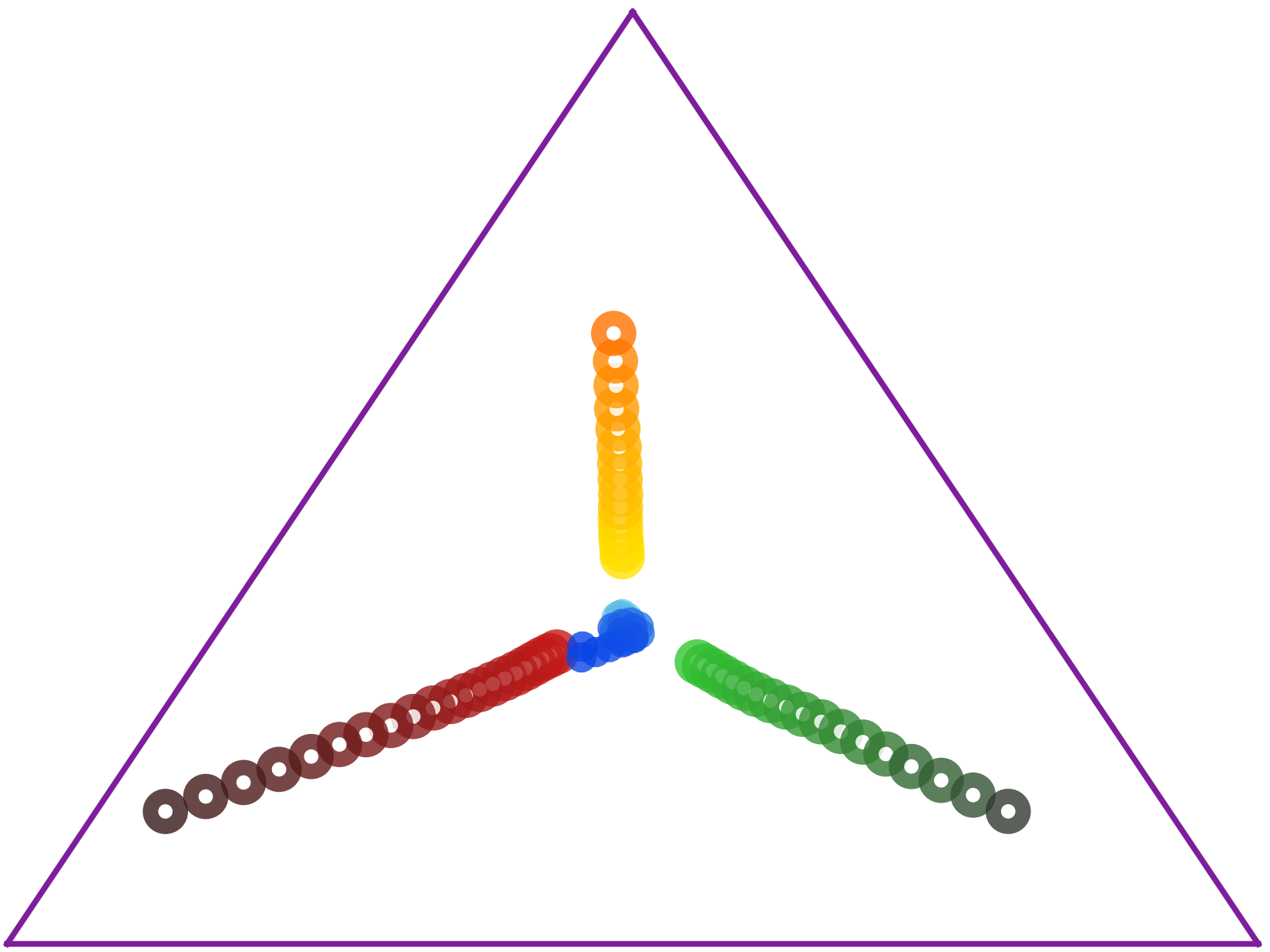
To visualize the policy evolution process, we use DIAYN [7] as our diversity algorithm and construct a simple 3-state MDP [8] to conduct the experiment. The set of feasible state marginal distributions is described by a triangle in . And we use state occupancy measure to represent policy . Moreover, we project the state occupancy measure onto a two-dimensional simplex for visualization.
Let be the average state marginal distribution of all policies. Figure 1(a) shows policy evolution during training. Initially, the state occupancy measures of different policies are similar. However, as training progresses, the policies spread out, indicating increased diversity. Figure 1(a) highlights that diversity [8] ensures distinct state occupancy measures among policies.
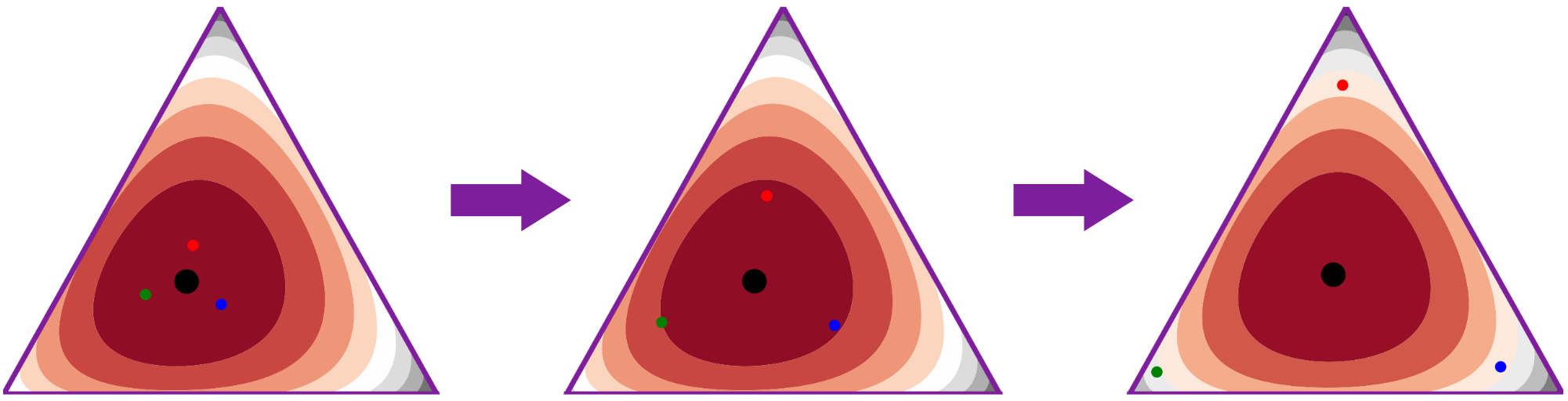
We use to denote mutual information. The diversity metric in unsupervised skill discovery algorithms is based on the mutual information of states and latent variable . Furthermore, the mutual information can be viewed as the average divergence between each policy’s state distribution and the average state distribution [8]:
| (6) |
Figure 1(b) shows the policy evolution process and the diversity metric . We find that the diversity metric increased gradually during the training process, which is in line with our expectation.
5.2 Policy Selection Ablation
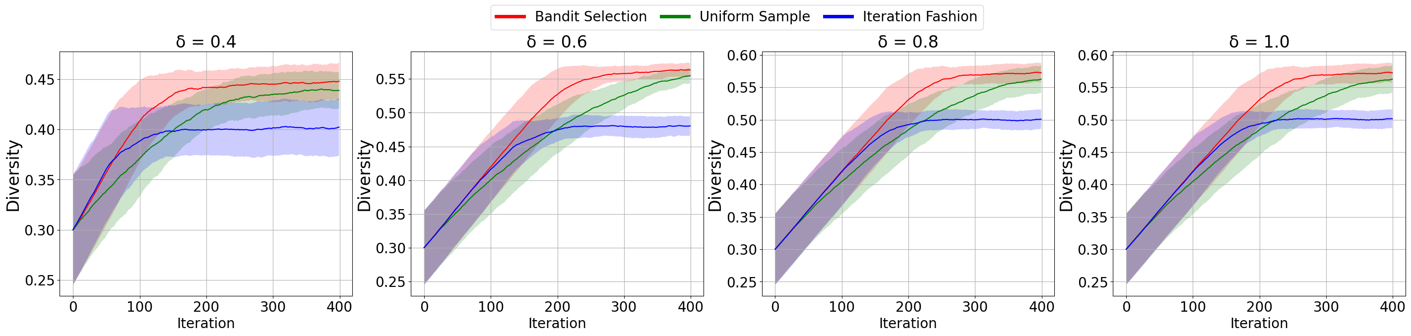
We continue to use 3-state MDP [8] as the experimental environment. Whereas, in order to get closer to the complicated practical environment, we set specific -target and increased the number of policies. Moreover, when a policy that hasn’t met the diversity requirement is chosen to update, we will receive a reward , otherwise, we will receive a reward . We use as the diversity metric and use LinUCB[14] as our contextual bandit algorithm.
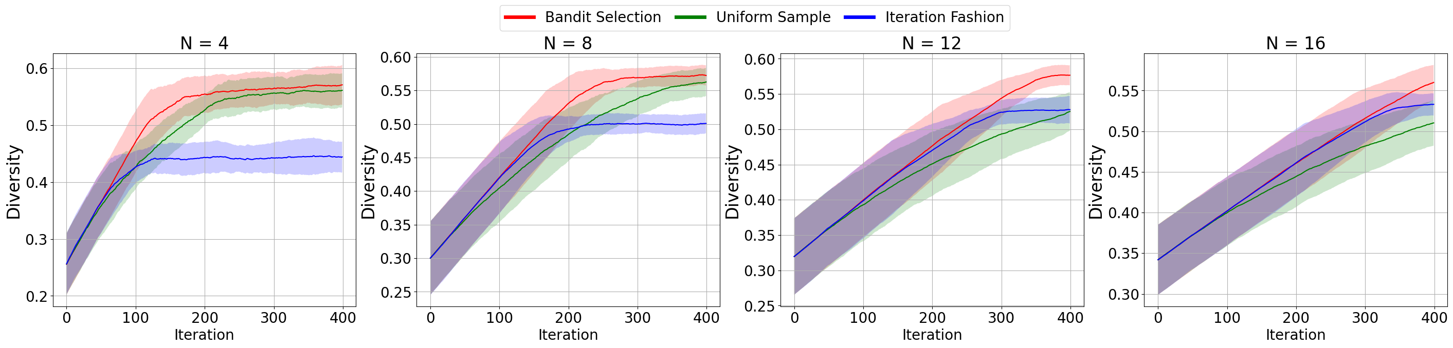
Figure 2 shows the training curves under different numbers of policies and different -target over six random seeds. The results show that bandit selection not only always reaches the convergence fastest, but also achieves the highest overall diversity metric of the population when it converges. We now empirically analyze the reasons for this result:
Drawbacks of uniform sample. In many experiments, we observe that uniform sample has similar final performance to bandit selection, but significantly slower convergence. This is because after several iterations, some policies become distinct enough to prioritize updating other policies. However, uniform sample treats all policies equally, resulting in slow convergence.
Drawbacks of iteration fashion. In experiments, the iteration fashion converges quickly but has lower final performance than the other two methods. It’s greatly affected by initialization. Each policy update depends on the previous one, so poor initialization can severely impact subsequent updates, damaging the overall training process.
Advantages of bandit selection. Considering historical rewards and balancing exploitation and exploration, bandit selection quickly determines if a policy is different enough to adjust the sample’s probability distribution. Unlike iteration fashion, all policies can be selected for an update in a single iteration, making bandit selection not limited by policy initialization.
6 Conclusion
In this paper, we compare existing diversity algorithms, provide a unified diversity reinforcement learning framework, and investigate the convergence of training diverse policies. Moreover, we propose bandit selection under our proposed framework, and present the regret bound for it. Empirical results indicate that bandit selection achieves the highest diversity score with the fastest convergence speed compared to baseline methods. We also provide a geometric perspective on policy evolution through experiments. In the future, we will focus on the comparison and theoretical analysis of different reward calculation methods. And we will continually explore the application of diversity RL algorithms in more real-world decision-making tasks.
References
- [1] Auer, P.: Using confidence bounds for exploitation-exploration trade-offs. Journal of Machine Learning Research 3(Nov), 397–422 (2002)
- [2] Auer, P., Cesa-Bianchi, N., Fischer, P.: Finite-time analysis of the multiarmed bandit problem. Machine learning 47(2), 235–256 (2002)
- [3] Berner, C., Brockman, G., Chan, B., Cheung, V., Debiak, P., Dennison, C., Farhi, D., Fischer, Q., Hashme, S., Hesse, C., et al.: Dota 2 with large scale deep reinforcement learning. arXiv preprint arXiv:1912.06680 (2019)
- [4] Chen, W., Huang, S., Chiang, Y., Chen, T., Zhu, J.: Dgpo: Discovering multiple strategies with diversity-guided policy optimization. In: Proceedings of the 2023 International Conference on Autonomous Agents and Multiagent Systems. pp. 2634–2636 (2023)
- [5] Chu, W., Li, L., Reyzin, L., Schapire, R.: Contextual bandits with linear payoff functions. In: Proceedings of the Fourteenth International Conference on Artificial Intelligence and Statistics. pp. 208–214. JMLR Workshop and Conference Proceedings (2011)
- [6] Ellis, B., Moalla, S., Samvelyan, M., Sun, M., Mahajan, A., Foerster, J.N., Whiteson, S.: Smacv2: An improved benchmark for cooperative multi-agent reinforcement learning. arXiv preprint arXiv:2212.07489 (2022)
- [7] Eysenbach, B., Gupta, A., Ibarz, J., Levine, S.: Diversity is all you need: Learning skills without a reward function. In: International Conference on Learning Representations (2018)
- [8] Eysenbach, B., Salakhutdinov, R., Levine, S.: The information geometry of unsupervised reinforcement learning. In: International Conference on Learning Representations (2021)
- [9] Fu, W., Du, W., Li, J., Chen, S., Zhang, J., Wu, Y.: Iteratively learning novel strategies with diversity measured in state distances. Submitted to ICLR 2023 (2022)
- [10] Huang, S., Chen, W., Zhang, L., Li, Z., Zhu, F., Ye, D., Chen, T., Zhu, J.: Tikick: Towards playing multi-agent football full games from single-agent demonstrations. arXiv preprint arXiv:2110.04507 (2021)
- [11] Huang, S., Yu, C., Wang, B., Li, D., Wang, Y., Chen, T., Zhu, J.: Vmapd: Generate diverse solutions for multi-agent games with recurrent trajectory discriminators. In: 2022 IEEE Conference on Games (CoG). pp. 9–16. IEEE (2022)
- [12] Kumar, S., Kumar, A., Levine, S., Finn, C.: One solution is not all you need: Few-shot extrapolation via structured maxent rl. Advances in Neural Information Processing Systems 33, 8198–8210 (2020)
- [13] Lanctot, M., Zambaldi, V., Gruslys, A., Lazaridou, A., Tuyls, K., Pérolat, J., Silver, D., Graepel, T.: A unified game-theoretic approach to multiagent reinforcement learning. Advances in neural information processing systems 30 (2017)
- [14] Li, L., Chu, W., Langford, J., Schapire, R.E.: A contextual-bandit approach to personalized news article recommendation. In: Proceedings of the 19th international conference on World wide web. pp. 661–670 (2010)
- [15] Liu, X., Jia, H., Wen, Y., Yang, Y., Hu, Y., Chen, Y., Fan, C., Hu, Z.: Unifying behavioral and response diversity for open-ended learning in zero-sum games. arXiv preprint arXiv:2106.04958 (2021)
- [16] Mahajan, A., Rashid, T., Samvelyan, M., Whiteson, S.: Maven: Multi-agent variational exploration. arXiv preprint arXiv:1910.07483 (2019)
- [17] Makoviychuk, V., Wawrzyniak, L., Guo, Y., Lu, M., Storey, K., Macklin, M., Hoeller, D., Rudin, N., Allshire, A., Handa, A., et al.: Isaac gym: High performance gpu-based physics simulation for robot learning. arXiv preprint arXiv:2108.10470 (2021)
- [18] May, B.C., Korda, N., Lee, A., Leslie, D.S.: Optimistic bayesian sampling in contextual-bandit problems. Journal of Machine Learning Research 13, 2069–2106 (2012)
- [19] Osa, T., Tangkaratt, V., Sugiyama, M.: Discovering diverse solutions in deep reinforcement learning by maximizing state–action-based mutual information. Neural Networks 152, 90–104 (2022)
- [20] Shi, J.C., Yu, Y., Da, Q., Chen, S.Y., Zeng, A.X.: Virtual-taobao: Virtualizing real-world online retail environment for reinforcement learning. In: Proceedings of the AAAI Conference on Artificial Intelligence. vol. 33, pp. 4902–4909 (2019)
- [21] Wang, T.T., Gleave, A., Belrose, N., Tseng, T., Miller, J., Dennis, M.D., Duan, Y., Pogrebniak, V., Levine, S., Russell, S.: Adversarial policies beat professional-level go ais. arXiv preprint arXiv:2211.00241 (2022)
- [22] Watkins, C.J.C.H.: Learning from delayed rewards. Robotics & Autonomous Systems (1989)
- [23] Xue, W., Cai, Q., Zhan, R., Zheng, D., Jiang, P., An, B.: Resact: Reinforcing long-term engagement in sequential recommendation with residual actor. arXiv preprint arXiv:2206.02620 (2022)
- [24] Yu, C., Yang, X., Gao, J., Yang, H., Wang, Y., Wu, Y.: Learning efficient multi-agent cooperative visual exploration. arXiv preprint arXiv:2110.05734 (2021)
- [25] Zahavy, T., O’Donoghue, B., Barreto, A., Flennerhag, S., Mnih, V., Singh, S.: Discovering diverse nearly optimal policies with successor features. In: ICML 2021 Workshop on Unsupervised Reinforcement Learning (2021)
- [26] Zhou, Z., Fu, W., Zhang, B., Wu, Y.: Continuously discovering novel strategies via reward-switching policy optimization. In: International Conference on Learning Representations (2021)