DMFT reveals the non-Hermitian topology in heavy-fermion systems
Abstract
We find that heavy fermion systems can have bulk “Fermi arcs”, with the use of the non-Hermitian topological theory. In an interacting electron system, the microscopic many-body Hamiltonian is Hermitian, but the one-body quasiparticle Hamiltonian is non-Hermitian due to the finite quasiparticle lifetime. We focus on heavy electron systems as a stage of finite lifetime quasiparticles with two lifetimes, since quasiparticle lifetimes for f-electrons and c-electrons should be different. Two lifetimes induce exceptional points (EPs) of the non-Hermitian quasiparticle Hamiltonian matrix in momentum space. The line connecting between two EPs characterizes the bulk Fermi arcs. With the use of the dynamical mean field theory (DMFT) calculation, we confirm our statement in Kondo insulators with a momentum-dependent hybridization in two-dimensions. We show that the concept of the EPs in the non-Hermitian quasiparticle Hamiltonian is one of powerful tools to predict new phenomena in strongly correlated electron systems.
Introduction —
A standard theory for metals describes Fermi surfaces that are manifolds with codimension-one [closed loops in two dimensions (2D) and closed surfaces in three dimensions (3D)] in momentum space. In semimetals, there are codimension-two Fermi nodes and band crossings: nodal points in 2D and nodal lines in 3D, respectively. However, the pseudogap phase of hole-doped cuprate high- superconductors exhibits Fermi arcs, which are opened Fermi surfaces with endpoints.Keimer .
In recent worksHuitao ; Vlad ; Papaj , it was revealed that nodal points in 2D Dirac semimetals can become Fermi arcs, the locations of which are determined by a topological theory of finite-lifetime quasiparticles. In quantum many-body systems, quasiparticles generically have finite lifetimes, resulting from scattering. Hence, they are described by non-Hermitian Hamiltonians, whose imaginary part reflects the finite lifetimes. These non-Hermitian matrices can have topological features called the “exceptional points” (EPs), where the Hamiltonian becomes non-diagonalizableKato . It was then shownHuitao ; Vlad ; Papaj that the existence of EPs lead to Fermi arcs, which end on the EPs. In previous studies, it was shown that two-lifetime modelsVlad , where two electron bands with finite hybridization have different lifetimes originating from the electron-phonon scattering, often have EPs and thus also Fermi arcs. Elastic electron-impurity scattering also induces EPs and Fermi arcsPapaj .
In this work, we demonstrate how two distinct lifetimes due to electron-electron interaction naturally appear in heavy fermion systems. Heavy-fermion systems can be described by the periodic Anderson modelTsunetsugu . This model naturally features two lifetimes, since there are two kinds of electrons, itinerant -electrons and localized -electrons. The -electrons feel much stronger electron-electron interaction than the -electrons, which leads to different lifetimes of the two bands.
We show that a Kondo semimetal, a Kondo lattice system with a small energy gap such as CeNiSnNakamoto , naturally has Fermi arc. The Kondo semimetal is understood as a Kondo insulator with a momentum-dependent hybridization gap. A Kondo insulator exhibits an insulating behavior at low temperatures, since the volume of the Fermi surface counts both - and -electrons and the hybridization of the Fermi surfaces makes this system gapped. However, it exhibits a metallic behavior with a -electron Fermi surface at high temperatures, since the contribution from the -electrons is blurred due to its finite lifetime, which decreases as the temperature raisesPColeman . The characteristic crossover temperature between the two behaviors is determined by comparing the magnitude of the hybridization gap and the temperature-dependent inverse lifetime of the -electron. As we will show, in the Kondo semimetal with a momentum-dependent gap, the crossover happens at different temperatures for different points on the Fermi surface. Thus, a Kondo semimetal has a Fermi arc, which is a partial Fermi surface ending on EPs.
In this paper, we study a periodic Anderson model with a momentum-dependent hybridization gap in two dimensions. Using a perturbation theory, we argue that the difference between electron correlations in - and -bands naturally lead to two lifetimes (in fact, under certain assumptions, the self-energy of -electrons vanishes to all orders of perturbations), which results in EPs and Fermi arcs at certain temperatures. To confirm our statement numerically, we adopt the dynamical mean field theory (DMFT) with the numerically exact continuous-time quantum Monte Carlo solver. The spectral function calculated by the DMFT clearly shows that there is the Fermi arc defined by the region where the spectral function has a peak at zero energy. These Fermi arcs due to the EPs can be observed by angle-resolved photoemission spectroscopy (ARPES).
Exceptional points of the quasiparticle Hamiltonian —
We introduce the EPs and the finite-lifetime quasiparticle Hamiltonian for strongly correlated electron systemsHuitao ; Vlad .
We first introduce quasiparticle Hamiltonian :
| (1) |
which can be extracted from the retarded electron Green’s function , where is the single-particle Hamiltonian and is the electron’s self-energy that includes the effect of electron-electron interaction. Note that the quasiparticle Hamiltonian can be non-Hermitian and that its spectrum can be complex: In general, is a sum of the Hermitian part and the non-Hermitian part : . renormalizes the bare band structure, while leads to finite quasiparticle lifetimes, resulting in the non-Hermitian self-energy and HamiltonianHuitao ; Vlad . The spectrum determines the complex poles of the Green’s function according to . In the vicinity of a first-order pole, the Green’s function takes the form . The real part of determines the quasiparticle’s dispersion, while its imaginary part defines the quasiparticle’s inverse lifetime.
The important difference between Hermitian and non-Hermitian Hamiltonians is that the latter can be non-diagonalizable at certain momenta. Those points are called “exceptional points” in the mathematical physics literatureKato . At the EPs, linearly independent eigenstates do not span the full Hilbert space. One of the authors showed that these EPs in two and higher dimensions are topologically stableHuitao .
Topological exceptional points can appear in the quasiparticle spectrum of zero- and small-gap materials such as Dirac semimetals in two dimensionsVlad . We show that this scenario is also applicable to heavy Fermion systems, where the two orbitals correspond to itinerant and localized electrons and the hybridization gap can have a momentum-dependent form factorIkedaMiyake ; Dzero ; Zhong .
|
Self-energy in heavy fermion systems —
Let us now demonstrate how two different lifetimes naturally occur in heavy fermion systems. We discuss how the self-energy leads to EPs and Fermi arcs, when combined with a momentum-dependent hybridization gap. We consider a periodic Anderson model (PAM) defined as
| (5) |
where
| (8) |
and . Here, () is an annihilation operator for itinerant - (localized -) electron with momentum and spin , with dispersions and , respectively. We use as the unit of the energy scale hereafter, and here is the chemical potential. We consider the case of half filling, which corresponds to and , and is characterized by the particle-hole symmetry. At half filling, the term is exactly cancelled by the Hartree part of the electron’s self-energy, so we omit it for the rest of the paper for brevity. The hybridization gap is expressed as for -wave case which describes the Kondo insulators and for -wave case which describes Kondo semimetals, respectively. In this work, we focus on the -wave gap, which has point nodes on the Fermi surface at sup .
It is known that the PAM exhibits a number of strongly correlated phenomena showing the non-Fermi-liquid behavior Amaricci2008 and undergoing the Mott transition Sordi2007 ; Amaricci2017 ; Amaricci2012 near some particular fillings. In our work, we stay away from these special fillings, i.e., in the regime where the Fermi liquid description remains adequate.
Due to the fact that the electrons in model (5) are not interacting, only electrons have a finite lifetime: This implies the following form of
| (9) |
This point is explained in Sec. S2. in the supplemental material. Thus, the two-lifetime description naturally arises in the periodic Anderson model.
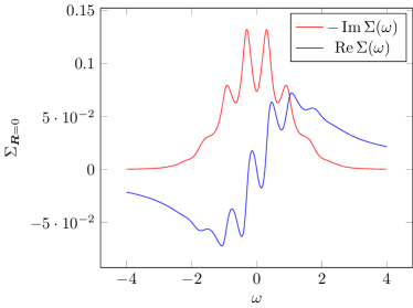
The -electron self-energy is computed using a second-order perturbation theory in Sec. S2 of the supplemental material (see also, Ref. Yamada1986 ). At temperatures comparable or higher than the hybridization scale , we can ignore the momentum dependence of . This is because the finite-temperature broadening renders the -band approximately flat. Hence, the onsite interaction and a flat band together result in a local self-energy. Since we are interested in the spectrum of low-energy electron excitations, we focus on low-frequency self energies. In particular, in the zero-frequency limit, can be treated as a purely imaginary constant, , where the real part vanishes because the particle-hole symmetry pins the energy of the -electron at zero. Furthermore, at small frequencies, one can expand as the following:
| (10) |
Our DMFT calculations presented later show that coefficients and are generally positive. The inclusion of the positive higher-order terms and will not change the qualitative features of the electron spectrum function discussed next. In particular, the effective of including , which is the leading term of the real part of , is a reduction of the widths of some bands: it renormalizes to , to , and to , respectively, while keeping unaffected. (This is analyzed in details in Sec. S2 of the SM.) Here, .
Bulk Fermi arcs —
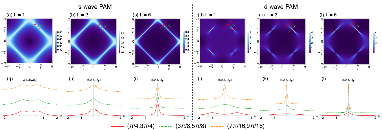
We now discuss the electron spectral function, and show the Fermi arcs in the -wave PAM. We plot the electron spectral function from (1). The result is shown in Fig. 1.
In general, the inverse lifetime is small at low temperatures and large at high temperatures, reflecting a long and a short quasiparticle lifetime, respectively. Hence, we demonstrate low-temperature and high-temperature phenomena using , and , respectively. In the -wave PAM, there is a gap with in the whole momentum space as shown in Figs.1(a) and (g). With increasing , the gap is closed on a Fermi surface. This is the standard crossover behavior between a Kondo insulator at a low temperature and a small -electron Fermi surface at a high temperature. In the -wave PAM, on the other hand, we can clearly see the bulk Fermi arcs at the low temperature, as shown in Figs.1(d) and (j). The Fermi arcs grow into a full -electron Fermi surface at the high temperature.
The Fermi arcs observed in the -wave PAM can be explained as follows. With , the complex poles of the Green’s function are given by
| (11) |
with . This complex spectrum is similar to that for the Dirac semimetals in two dimensions if we replace and with and , respectively (and assuming )Vlad .
The spectral function with is given by
| (12) |
with
| (13) |
The form-factors and originate from the non-zero real part of self-energy, and both equal to 1 in case when .
We see that the spectral function is given by the sum of two Lorentzians, whose locations and widths are given by the real and imaginary parts of , respectively. In particular, we focus on the line , which is the location of the high-temperature -electron Fermi surface. Along this line, Eq. (11) is simplified to the following form,
| (14) |
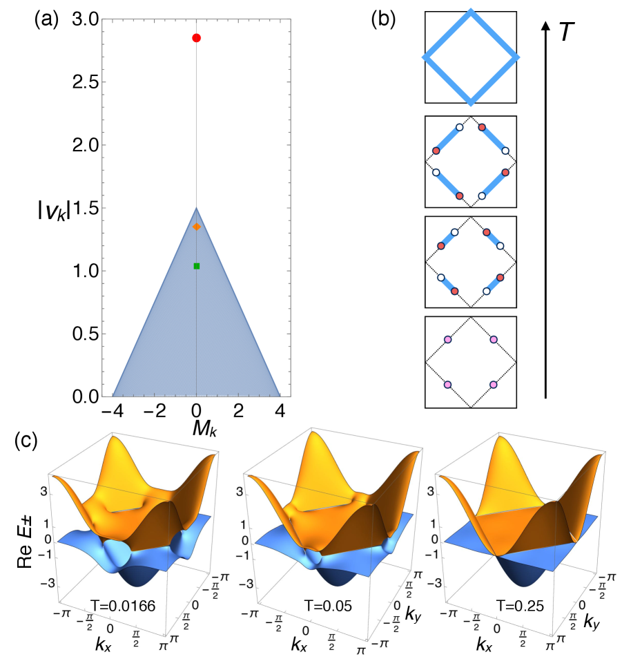
We first focus at a fixed momentum , and discuss how a temperature-dependent affects the electron spectrum function. For simplicity, we consider (). In general, we expect to increase with temperature. In particular, it should approach zero in the limit. The competition between the temperature-dependent and the hybridization can explain the Kondo crossover. At low temperatures, when , have different real parts, and the spectrum is a superposition of two peaks. The distance between the two peaks, , represents a hybridization gap. This indicates that the and electrons are hybridized, and the electrons join the electrons to contribute to the volume of the Fermi surface. At high temperature, when , have the same real part, and the spectrum exhibits a single peak located at if . This indicates that there is no gap, and is on a Fermi surface. This also means that the -electrons form local moments, which are detached from the Fermi surface formed solely by the electron.
For the -wave PAM, the crossover between the two behaviors happens at the same temperature where for all , and a complete -electron Fermi surface emerges from a Kondo insulator as the temperature raises. For the -wave PAM, however, at different momenta on the Fermi surface, the crossover happens at different temperatures determined by . In particular, for , the Fermi surface is separated into two regions by EPs located at , where become degenerate. The hybridization gap only appears on part of the crossing lines, where . The rest of the crossing lines, where , then forms Fermi arcs. Hence, the arcs are longer with bigger . At zero temperature, the model is a Kondo semimetal with point nodes. As temperature raises and increases, the Fermi arcs grow longer, until the full -electron Fermi surface emerges at .
We notice that, phenomenologically, when two peaks in the spectrum function are closer than their peak widths, they become inseparable experimentally. Hence, the exact locations of the ending points of the Fermi arcs may differ from the EPs, and they depend on the details of data analysis. However, the existence of the Fermi arcs is tied to EPs in the quasiparticle Hamiltonian.
|
Dynamical Mean Field Theory —
To treat the heavy fermion systems more accurately, we use the dynamical mean field theory (DMFT). In the DMFT, we assume that the self-energy does not depend on the momentum:
| (15) |
This assumption is appropriate when the temperature is not too low comparison with the maximum of hybridization energysup . The momentum dependence does not affect the appearance of the bulk Fermi arcs, qualitatively. We set and . To calculate the local and momentum-dependent spectral functions and , we utilize the DMFT with the numerically exact segment-based hybridization-expansion continuous-time quantum Monte Carlo impurity solver (ct-HYB) Werner . We point out that there is no fermion sign problem because of the off-diagonal elements of the self-energy in the spin space are zero in our two-orbital systemNagaiDMFT . After confirming that the self-energy for electrons is zero in the two-orbital DMFT calculation, we use one-orbital DMFT calculation with integrating out the -electron degree of freedom. Here, the effective impurity problem is solved by an open-source program package, QISTiqist . We set .
|
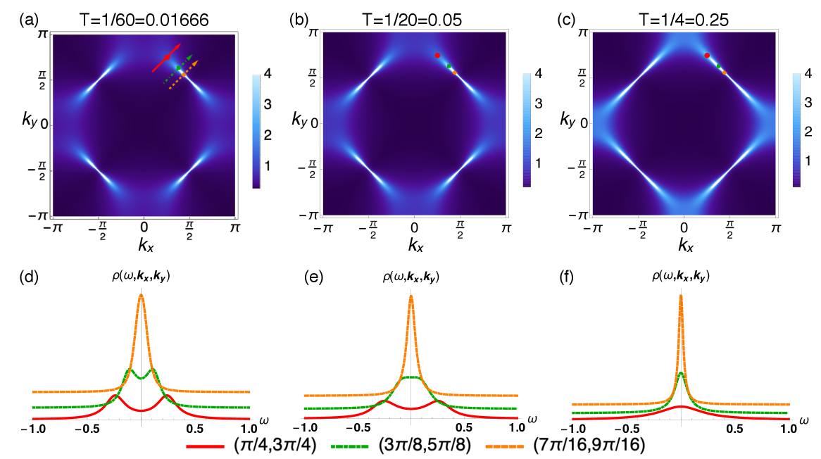
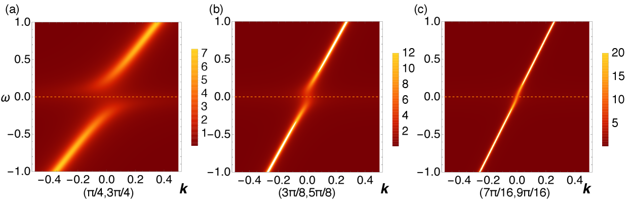
Figure 3 shows the spectral functions and the Fermi arcs. To calculate the real-frequency self-energy and the spectral function , we use the Padé approximation as the method for the numerical analytic continuation of the self-energy . After the Padé approximation, we fit the self-energy with the form in the region . We find that the set of parameters equals (5.70895, 2.28419, 1.01368, 1.15838, 0.580893) at , (2.70929, 9.54693, 5.49701, -2.19662, 5.38239) at , and (2.06142, 11.8766, 16.49, -10.2929, -6.21199) at , respectively. Along the Fermi line without hybridization defined by close to and , the spectral function begins to have a dip at by decreasing temperature, as shown in Fig. 3(d)-(f). We confirm that the spectral functions as a function of and show that there is a gap at zero energy in the low temperature region. These results indicate the existence of the Fermi arc, since the line where the spectral function has a peak at the zero energy has boundaries.
Summary —
In this work, we studied heavy-electron systems using PAMs. Although the microscopic many-body Hamiltonian is Hermitian, the one-body quasiparticle Hamiltonian is non-Hermitian because of finite quasiparticle lifetimes, which is due to electron interactions. In particular, we demonstrate that the difference in electron correlations between - and -electrons in PAMs naturally leads to two lifetimes in the non-Hermitian quasiparticle Hamiltonian. This, combined with a -wave hybridization gap, leads to the existence of EPs in the Hamiltonian and “Fermi arcs” in electron spectral function, at suitable temperatures. Our DMFT calculation with a numerically exact continuous-time quantum Monte Carlo solver confirmed our statement. These unusual Fermi arcs due to EPs can be observed by ARPES, which measures electron spectral function. Our discussion is applicable to other systems, such as two- and three-dimensional Kondo insulators with -wave hybridization. In a two-dimensional system with -wave hybridization ( with ), cross-shaped Fermi arcs appear around and . In a three-dimensional system, the Fermi arc becomes the three-dimensional “Fermi arc” defined by the surface with the boundaries in momentum space, which will be shown elsewhere.
Acknowledgment —
Y.N. would like to acknowledge H. Shen for helpful discussions and comments. The calculations were performed by the supercomputing system SGI ICE X at the Japan Atomic Energy Agency. YN was partially supported by JSPS KAKENHI Grant Number 15K00178 and 18K03552, the ”Topological Materials Science” (No. JP16H00995 and No. 18H04228) KAKENHI on Innovative Areas from JSPS of Japan. V. K. was partially supported by the Quantum Materials program at LBNL, funded by the US Department of Energy under Contract No. DE-AC02-05CH11231.
Y.N. and Y.Q. contributed equally to this work.
Note added —
Recently, we learned about the related works Yoshida and Michishita
References
- (1) B. Keimer, S. A. Kivelson, M. R. Norman, S. Uchida and J. Zaanen, From quantum matter to high-temperature superconductivity in copper oxides, Nature 518, 179 (2015).
- (2) H. Shen, B. Zhen, and L. Fu, Topological Band Theory for Non-Hermitian Hamiltonians, Phys. Rev. Lett. 120, 146402 (2018).
- (3) V. Kozii and Liang Fu, Non-Hermitian Topological Theory of Finite-Lifetime Quasiparticles: Prediction of Bulk Fermi Arc Due to Exceptional Point, arXiv:1708.05841.
- (4) M. Papaj, H. Isobe, and L. Fu, Bulk Fermi arc of disordered Dirac fermions in two dimensions, Phys. Rev. B 99, 201107 (2019).
- (5) T. Kato, Perturbation theory of linear operators (Springer, Berlin, 1966).
- (6) H. Tsunetsugu, M. Sigrist, and K. Ueda, The ground-state phase diagram of the one-dimensional Kondo lattice model, Rev. Mod. Phys. 69, 809 (1997).
- (7) G. Nakamoto, T. Takabatake, H. Fujii, A. Minami, K. Maezawa, I. Oguro, and A. A. Menovsky, Crystal Growth and Characterization of the Kondo Semimetal CeNiSn, J. Phys. Soc. Jpn. 64, 4834 (1995).
- (8) P. Coleman, Many-Body Physics: From Kondo to Hubbard (eds E. Pavarini, E. Koch and P. Coleman), Chapter 1, 1.1-1.34 (2015), Forschungszentrum Julich, 2015.
- (9) H. Ikeda and K. Miyake, A Theory of Anisotropic Semiconductor of Heavy Fermions, J. Phys. Soc. Jpn. 65, 1769 (1996).
- (10) Y. Zhong, Y. Liu, and H.-G. Luo, Topological phase in 1D topological Kondo insulator: Z2 topological insulator, Haldane-like phase and Kondo breakdown, Eur. Phys. J. B 90, 147 (2017).
- (11) M. Dzero, K. Sun, V. Galitski, and P. Coleman, Topological Kondo Insulators, Phys. Rev. Lett. 104, 106408 (2010).
- (12) See Supplemental Material at [URL will be inserted by publisher] for the technical details of the perturbation analysis and the DMFT calculation.
- (13) A. Amaricci, G. Sordi, and M. J. Rozenberg, Non-Fermi-Liquid Behavior in the Periodic Anderson Model, Phys. Rev. Lett. 101, 146403 (2008).
- (14) G. Sordi, A. Amaricci, and M. J. Rozenberg, Metal-Insulator Transitions in the Periodic Anderson Model, Phys. Rev. Lett. 99, 196403 (2007).
- (15) A. Amaricci, L. de’ Medici, G. Sordi, M. J. Rozenberg, and M. Capone, Path to poor coherence in the periodic Anderson model from Mott physics and hybridization Phys. Rev. B 85, 235110 (2012)
- (16) A. Amaricci, L. de’ Medici and M. Capone, Mott transitions with partially filled correlated orbitals, Euro Phys. Lett. 118, 17004 (2017).
- (17) K. Yamada and K. Yosida, Fermi liquid theory on the basis of the Periodic Anderson Hamiltonian, Prog. Theo. Phys., 76 621 (1986).
- (18) P. Werner and A. J. Mills, Hybridization expansion impurity solver: General formulation and application to Kondo lattice and two-orbital models, Phys. Rev. B 74, 155107 (2006).
- (19) Y. Nagai, S. Hoshino, and Y. Ota, Critical temperature enhancement of topological superconductors: A dynamical mean-field study, Phys. Rev. B 93, 220505(R) (2016).
- (20) L. Huang, Y. Wang, Z. Y. Meng, L. Du, P. Werner, and X. Dai, iQIST: An open source continuous-time quantum Monte Carlo impurity solver toolkit, Comput. Phys. Commun. 195, 140 (2015).
- (21) T. Yoshida, R. Peters, and N. Kwakami, Non-Hermitian perspective of the band structure in heaby-fermion systems. Phys. Rev. B 98, 035141 (2018).
- (22) Y. Michishita, T. Yoshida, and R. Peters, Relation between exceptional points and the Kondo effect in f-electron materials, Phys. Rev. B 101, 085122 (2020).
Supplemental material for “DMFT reveals the non-Hermitian topology in heavy-fermion systems”
S1. Density of states from the vicinity of a Dirac node
The energy dispersion near a node located at is described by the effective Hamiltonian to the first order in :
| (S1) |
The axes are rotated by for convenience and we find the correspondence , , and . It can be interpreted as follows: The direction is chosen to be perpendicular to the Fermi surface, along which hybridization is absent. It corresponds to the – direction. Then, is parallel to the Fermi surface and it describes the hybridization of the two bands. The two different bands allows the parameter , describing the tilt of the Dirac cone. Along the direction, the slower velocity of the first component corresponds to the band, and the faster to the band. The off-diagonal terms represent hybridization of the two bands.
The local density of states is obtained by
| (S2) |
with the retarded Green’s function
| (S3) |
Here we assume that the self-energy takes the form
| (S4) |
Without a trace of matrices, we can extract the contribution from each band. When the self-energy is independent of momentum , we can evaluate the momentum integration to obtain
| (S5) |
where is the high-energy cutoff and is defined by
| (S6) |
We note that the expression of is valid for and .
When the self-energy vanishes, we find an expression for free Dirac fermions, i.e., . In contrast, a finite imaginary part of the self-energy makes the density of states finite at : .
S2. The effect of on the dispersion
In this section, we study the effect of , which is the coefficient of the linear- term in the real part of the -electron self-energy [see Eq. (10) in the main text]. We argue that the effect of including can be absorbed into renormalizing the parameters , , and in electron’s Green’s function. To see this, we consider the Green’s function determined by including the -electron self-energy ,
| (S7) |
As discussed in the main text, the electron spectral function can be decomposed into Lorentzian peaks, which are determined by poles of [see Eq. (12)]. The poles of are the solutions of , which can be rewritten as the following form,
| (S8) |
Hence, we see that , and are normalized to , and , respectively.
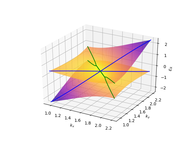
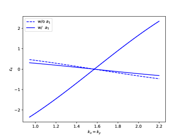
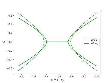
The effect of is illustrated in Fig. S1, which shows the dispersion of the quasiparticle peaks with and without . One can see that, after including , the bandwidth of -electron and the hybridization gap becomes smaller, and the Fermi arc, defined by Eq. (9) of the main text, becomes shorter, but the -electron band is not renormalized. To see the effect of , however, one has to consider the frequency dependence of the spectral function. Then, the exceptional points, which are the boundaries of the Fermi arcs, can be determined as points on the Fermi surface where starts having a dip at zero frequency instead of a peak, i.e, the zero-frequency peak splits into two peaks at finite frequencies, as shown in Figs. 1 (j)-(l) and 3 (d)-(f) of the main text. At zero frequency, on the other hand, the spectral function does not depend on (equivalently, on ) and is given by the following expression:
| (S9) |

S3. Self energy from the second-order perturbation theory
In this section, we compute the electron self-energy using a second-order perturbation theory in . In the perturbation theory, the self-energy is given by the one-particle-irreducible (1PI) diagrams. To the second order of , there are two such diagrams, shown in Fig. S2.


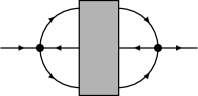
The perturbation theory shows that, since there is no interaction between -electrons in model (5), only -electrons have the self-energy. To see this, we notice that all fermion propagators in the self-energy diagrams in Fig. S2 are of fermions. This is because the interaction vertex, represented by the dot in the diagrams, only involves four electrons, since it comes from the onsite term in Eq. (5). Therefore, in the matrix of the self-energy, only the diagonal block of the electron is nonzero:
| (S10) |
In fact, this block structure even persists to all orders of perturbation. This is because all 1PI diagrams of orders higher than three can be represented by the schematic diagram in Fig. S2(c), where the self-energy bloc begins and ends with two vertices. Hence, the incoming and outgoing legs must be of electrons. Since the imaginary part of the non-Hermitian Hamiltonian in Eq. (1) comes solely from the imaginary part of the self-energy, the imaginary part also have this block structure: .
We first show that the first-order self-energy, represented by the diagram in Fig. S2(a), vanishes. It is straightforward to see that the first-order self-energy is independent of and , and does not have an imaginary part. Hence, it represents a constant energy shift of the electron, which must vanish because of the particle-hole symmetry in the model (5).
With the previous discussions, it becomes clear that only electron has a nontrivial self-energy, with corrections starting at second-order perturbations in . In the rest of this section, we will focus on the second-order self-energy of the electrons. Next, we argue that, due to the heaviness of the band, in the limit that the temperature is much larger than the width of the band , the self-energy is approximately momentum-independent.
To proceed, it is convenient to evaluate the Feynman diagram in Fig. S2(b) in real space. The real-space self-energy has the form Schweitzer1989 ; Schweitzer1990
| (S11) |
where is the Fermi-Dirac distribution function, and is the -electron density of state with the displacement , which can be read out from the bare Green’s function using the expression of in (8),
| (S12) |
the component, , represents the local density of state of the electron. In the Anderson lattice model (5), the electron has a narrow band, as , which is further broadened by the hybridization with the electrons. Therefore, the band width of the electron, , is of the order of . This is illustrated in Fig. S3, where is plotted. As shown in this figure, the density of state vanishes linearly at , because the dispersion has a node at ; starting from , the density of state increases until reaches a van Hove singularity. The density of state decreases pass that singularity, and further drops at another singularity. The majority of the density of state is within .
Now, we consider the limit . In this limit, is only nonvanishing at . In other words, the Fourier transform, , is momentum independent. This is because the momentum dependence of comes from the dispersion of electrons, as is the convolution of three -electron density-of-state functions in Eq. (S11). In the limit , the finite-temperature broadening is much larger than the bandwidth of -electron, and therefore smears out the momentum dependence in . The fact that is approximately momentum independent is confirmed by our numerical simulation: plotted in Fig. S4(b) indeed shows very weak momentum dependence. Therefore, in this paper, we ignore the momentum dependence of , and approximate .
Next, we discuss the frequency dependence of the self energy . Since it is a convolution of three , which has a bandwidth of , has a peak with width at the order of . Indeed, the numerical results of , shown in Fig. S4(b), shows a broad peak with a width on the order of . Besides the overall features at the scale of , , shown in Fig. S4(a), also exhibits oscillations, with the first peak appearing at the energy corresponding to the first van Hove singularity that appeared in the density of state shown in Fig. S3. This oscillation is an echo of the van Hove singularity, broadened because three functions are convoluted. In particular, focusing on close to zero, increases with . This can be understood by recalling that vanishes at , and increases as increases. Since is even in , it can be approximated as
| (S13) |
Correspondingly, decreases with for small omega. As an odd function of , it can be approximated by the following form for small ,
| (S14) |
Combining Eqs. (S13) and (S14) together, we obtain the following small-frequency expansion,
| (S15) |
Here, the positivity of the coefficients is a consequence of the vanishing density of state at . Therefore, we expect this to be a generic feature in models of Kondo insulators and semimetals with point nodes, both of which have .
S4. Spectral functions as a function of and
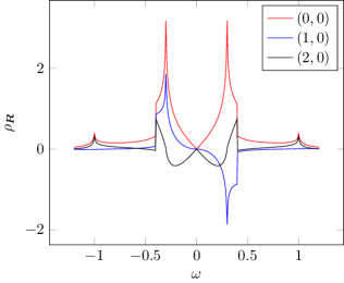
We show the spectral functions as a function of and obtained from the DMFT calculation, whose parameters are same as that in Fig.S5. The line cuts defined in Fig. 3(a) at .
|
S5. Temperature and hybridization dependence of the lifetime
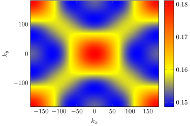
We show the temperature and hybridization dependence of the lifetime. The inverse lifetime is defined as . When is satisfied, the exceptional points in the momentum space appear as shown in Fig. 4(a) in the main text. Here, is a maximum value of the hybridization in the momentum space. Figure S6 shows that, at different hybridization strengths, the Fermi arcs appear at different temperatures.
|
References
- (1) H. Schweitzer and G. Czycholl, Zeitschrift für Physik B Condensed Matter 74, 303 (1989).
- (2) H. Schweitzer and G. Czycholl, Physica B: Condensed Matter 163, 415 (1990).